Investigation of Partition Function Transformation for the Potts Model into a Dichromatic Knot Polynomial 7₄

Abstract

This article examines quantum group symmetry using the Potts model. The transformation of the Potts model into a polynomial knot state on Kaufman square brackets is analyzed. It is shown how a dichromatic polynomial for a planar graph can be obtained using Temperley–Lieb operator algebra. The proposed work provides insight into the $7_4$ knot-partition function of Takara Musubi using a strain factor that represents the particles in the lattice knots of the above-mentioned model. As far as theoretical physics is concerned, this statement provides a correct explanation of the connection between the Potts model and the similar square lattice of knot and link invariants.

1. Introduction

Recently, there has been great concern about the partition function of the Potts model, which translates into topological combinatorics based on quantum group symmetry. For this reason, we adopt the symmetry point of view, owing to Landau’s contribution to science [1]. The modification of quantum symmetry in the model leads to variation in the phase transition.

The interaction symmetry and functional analysis of models (including the Potts model) of statistical mechanics builds on the constructional work of Jones [2]. This has led to the concept of internuncial subfactors within theoretical particle physics. Furthermore, Banica demonstrated that statistical mechanical models such as Jones’ originate from quantum groups [3]. Interest in this kind of research arose following Khovanov’s cohomology theory and its connection to the Potts model of statistical mechanics [4]. Homological Euler characteristics define a partition function based on Khovanov cohomology and the Potts model.

Graded cohomology groups have been constructed for each graph, for which the chromatic polynomial is on a planar graph [5,6,7,8,9,10]. This paper is based on earlier work on knot polynomials by Khovanov [11], the chromatic polynomial by Helme-Guizon and Rong [12], and the Tutte polynomial (for planar graphs) by Jasso-Hernandez and Rong [13].

Research into the Potts magnetic model and thermal properties of various two-dimensional lattices has important fundamental significance in physics. The Potts model models the energetic interactions of micro-scale nearest neighbors. Thus, in an intricate system, the conduct of the system is determined on a macro level. In the theory of phase transitions, this model plays a significant role. Consequently, in graded Khovanov homology theory for classical links, the use of graded Euler characteristics will result in the Jones polynomial [14,15,16]. Cohomology groups of Euler characteristics are a variant of the dichromatic polynomial [17].

We review the Potts model on a planar graph with ending area states and functions of graph vertices. A small modification argument of the model can lead to a sharp change in the symmetry elements; on certain occasions, the symmetry of the continuing group is unchanged, which means a change in the phase alteration. This provides compelling reasons to study the symmetry of quantum groups of physical models [18,19,20]. Quantum topological groups study operations on the vertices of a model or graph that are permutable with the Hamiltonian.

Accordingly, the dichromatic polynomials of $(2,n)$-torus knots are defined depending on the variables of the universal Tutte polynomial [21,22]. The models of Baxter are of great interest to researchers of the dichromatic Tutte polynomial in terms of mathematical physics [23,24,25,26,27,28,29,30,31,32,33].

At the beginning of the 21st century, scientists [34,35,36,37,38,39,40,41,42,43] searched for new methods of calculating the corresponding combinatorial polynomials that arise from the statistical mechanics of Bose gases. For example, Ref. [44] presented a statistical sum of a vertex model based on a directed planar graph.

Kauffman clearly explored exactly solvable vertex models with knot theory [45]. Semiclassical physics can reduce the limit of some abstract classical physics using anticommuting variables in the Potts model [46]. In the q-state Potts model, one assumes a choice of deformation coefficient value, such as $1,2,3,\dots ,q$ for each vertex G. Therefore, if G has N vertices, then there are $q^N$ states. The values of q can be the spins of elements at lattice knots, the types of metals in the fusion, etc. In [47,48,49,50], the statistical sum was calculated for the Potts model with different spins on square lattices. The study of bi-partite and tri-partite vertex models based on braid theory has led to the study of the invariant knot [51,52,53]. The partition function of dichromatic knot polynomial parameterization is an interpretation of Boltzmann weights on a planar graph. The value of $Z\left(X\right)$ allows the calculation of the main global parameters (temperature, total energy) and the study of phase transitions of a system (for instance, from a liquid to a solid state). If we generalize a regular lattice to an abstract graph, then the partition function of the q-state Potts model is equivalent to the Tutte polynomial [54,55].

Approaching combinatorics, each chord diagram of the $7_4$ knot can be associated with its own intersection graph. However, not every simple graph is a knot diagram graph. Coloring the vertices of a knot diagram allows the study of the dichromatic polynomial of a planar graph. Thus, we obtain a transition from a topological object-a knot to a combinatorial object-a graph. Using this transition, we can solve some topological problems using combinatorial methods.

This paper addresses the problem of learning a dichromatic polynomial and a $7_4$ knot-based Potts model by constructing a planar graph. The new result we want to highlight in this paper is the coloring of some regions of a planar graph. In addition, there is also the connection between the Potts model and the topological combinatorics of a planar graph. Thus, we define a close connection between the theory of graphs and knots.

Our goal is to obtain a new dichromatic knot polynomial. That will allow the determination of the chromatic states of each vertex of the knot diagram not described in [29]. Based on this dichromatic polynomial, it is possible to describe a quantum statistical interpretation of the chromatic states of each vertex of the knot diagram. Consequently, we check the amounts by state for knot $7_4$ by constructing a planar graph. For this purpose, Temperley–Lieb algebra and the Tutte polynomial were used. In this article, we present the correspondence between the partition function of the Potts model and the Tutte polynomial. Therefore, transforming the $7_4$ knot diagram into a graph will lead to remarkable synergies between the two research areas. The $7_4$ knot diagram is represented as a two-color (white and black states) graph in which there are many complex moves. Complex moves reduce the number of edges by one and cannot represent knots in a projection with a minimum number of intersections. The transition of 7-intersection knot diagrams to 4-valent graphs can expand the horizons of physics. This motivates the research of exactly solvable models, as per the Potts model and new dichromatic polynomials.

This work is presented as follows. The second part discusses the physical basis among the number of spin states in the Potts model and the probability of occurrence regarding a certain state of the graph knots. In the third section, the successive steps of finding the two-color polynomial of the $7_4$ knot are calculated by determining the chromatic state of the knot diagram. In the fourth section, the dichromatic $7_4$ knot polynomial from Takara Musubi is defined by coloring some regions of the planar graph. The partition function of the n function of the chiral Potts model is also considered through the corresponding variables and the deformation coefficient. The partition function associated with the planar graph G is calculated. In the general case, for a graph G with vertices $i,j,\dots$ and edges $〈i,j〉$, the partition function is equal to $Z_G(Q,T)={\sum }_{\sigma }{e}^{\left(\frac{-1}{kT}\right)E\left(S\right)}$. Where S passes through the states, $G,E\left(S\right)$ is the energy of the state, k is the Boltzmann constant, and T is the temperature.

2. The Partition Function of the Potts Model

In mathematical language, a knot is an embedding circle in 3-dimensional Euclidean space, $R^3$. A useful way to visualize and manipulate knots is to project the knot onto a plane: imagine the knot casting a shadow on a wall. A slight change in the direction of the projection will ensure one-to-one behavior, except at double points, called intersections, where the “shadow” of the knot intersects itself once in the transverse direction [55]. At each intersection, in order to recreate the original knot, it is necessary to distinguish the upper strand from the lower one. This is often done by breaking the strand running underneath. The resulting diagram is an immersed planar curve with additional information about which thread is on top and which is on the bottom at each intersection. These diagrams are called knot diagrams if they represent a knot and link diagrams if they represent a relationship [56].

For a set of q spins and Hamiltonian $h_i$ for $i=1$ or 2, the partition function of the q-state Potts model is

$$Z_i\left(G\right)=\sum exp(-\beta \left(h_i\left(\left(\omega \right)\right)\right).$$

(1)

Here, the summation is performed of all $\omega$ spins of groups G and $\beta =\frac{1}{kT}$, where T is the temperature of the system and $k=1.38\times {10}^{-23}$ $\mathrm{J}/\mathrm{K}$ is the Boltzmann constant. The above task is a standardization factor for the probabilistic Boltzmann partition. This $\varpi$ means that the probability of the system being in ardent steadiness against an abode of a certain shape with a degree of heating T is equal to

$$P_i(\varpi ,\beta )=\frac{exp(-\beta h_i\left(\varpi \right))}{\sum exp(-\beta \left(h_i\left(\left(\omega \right)\right)\right)}.$$

(2)

Boltzmann’s constant k provides a dimensionless magnitude of the exponent. Relatively, this causes $\beta ,K$, and T to all appear in the equal term, yet temperature appears as a relevant variable.

For example, Figure 1 shows all possible states of vertices in a graph with two rotation options (pitch black or colorless) where the whole lot peaks from $h_1\left(\varpi \right)=-11 \mathrm{J}$ and $h_2\left(\varpi \right)=13 \mathrm{J}$. Remarkably, applying a negative value $h_1$ counts edges with identical spins and $h_2$ computes edges with varied spins at the ends, thus a part of state $\varpi$$h_2\left(\varpi \right)=J\left|E\left(G\right)\right|+h_1\left(\varpi \right)$ [56].

In the following, we will have the opportunity to consider the generalization of K from real to complex values. Since it is natural to use two independent statements of the Potts model in inconsistent settings, the backing consideration of how one is merely a scalar factor against either supports the translation of notional decisions from one context to another. As an expeditious pattern, contemplate one rectangle. Despite two attainable rotations (light and pitch black), the nearby lattice is

$$\begin{array}{c}\hfill Z_2(G;q,\beta )=\sum exp(-\beta h_2\left(\varpi \right))=\\ \hfill =\sum exp(-\beta (J\left|E\left(G\right)\right|+h_1\left(\varpi \right)\left)\right)=exp(-K|E\left(G\right)\left|\right)Z_1(G;q,\beta ).\end{array}$$

(3)

The possible states (with accuracy up to rotation) and their Hamiltonian usage are shown in Figure 1.

So is the statistical sum is

$$\begin{array}{c}\hfill Z_1\left(G\right)=12exp\left(2K\right)+2exp\left(2K\right)+2.\end{array}$$

(4)

Against the expression for the possibility of the occurrence of a certain state, $\beta =\frac{1}{kT}$ is equal to $\frac{exp(-\beta h_i\left(\varpi \right))}{Z_i\left(G\right)}$. The most important thing is that these probabilities of the occurrence of a certain state and the use of their Hamiltonian depend on temperature. Extending the sample in Figure 1, we accept $J>0$, i. $J>0$, and argue the probability of a completely dark state at various temperatures. Given that J is positive, $h_1$ is used, with the all-pitch-black state existence of a solitary two-squat power state. If we suppose that ${\varpi }_b$ is the all-dark state, then the possibility that the system is in the all-dark state as a purpose of degree of heating is $P_r({\omega }_b,T)=\frac{exp\left(4K\right)}{\left(12exp\right(2K)+2exp(2K)+2)}$, where, as above, $K=\beta J$.

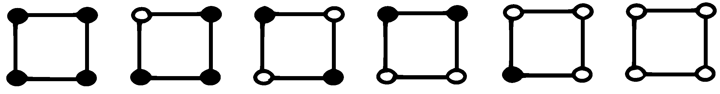
3. Finding the Dichromatic Polynomial by Constructing a Planar Graph

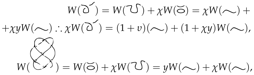
We determine the dichromatic polynomial as follows:

(5)

(6)

where $Z(•⨿)$ is the result of removing an edge from G while $G^{″}$ and of compressing that same edge so that its end knots have been crumpled to a single knot. In the second equation, • performs a graph against the knot and not the edges and $•⨿$ is the disjoint combination of the graph G.

Here, • indicates any connected shaded area and ⨿ shows an unconnected connection. If we define chromatic state S as any split of region U (knot shadow or link diagram) such that every vertex has been split, then the shading has $∥S∥$ numbers which are equal to the number of shaded regions, and $i\left(S\right)$ is equal to the quantity of internal vertex S. The sum of revolutions is expressed by the formula

$$Z\left(U\right)=\sum q^{∥S∥}{\upsilon }^{i\left(S\right)}={\displaystyle \sum _S^S}{q}^{\frac{1}{2}{(N-i\left(S\right)+\left|S\right|)}_{\upsilon }}i\left(S\right),$$

(7)

Let

$$W\left(U\right)=\sum _S(q^{\frac{1}{2}})\left|S\right|{(q^{\frac{1}{2}\upsilon })}^i\left(S\right),$$

(8)

Thus

$$Z\left(U\right)=q^{\frac{N}{2}}W\left(U\right).$$

(9)

The partitioning function involves counting the shaded areas against the loops in the connection diagram. The dichromatic polynomial is chosen so that the shaded part of the region is replaced by an alternating connection diagram, and the number of $∥S∥$ (shaded areas) is replaced by the number of components (grids) by S. The number of limit cycles for the shaded areas is $∥S∥$ where N indicates the number of double peaks, i.e., of the stroked range in U is consequently in monosemantic conformity, with the vertices of graph $G\left(U\right)$. Therefore, we claim that N is the sum of dual vertices and S is the chromatic state of U with $∥S∥$ coherent hatched regions and $i\left(S\right)$ interior vertices.

In the dichromatic polynomial, the extended state S in Figure 2 is given by the pair $S=(q,\upsilon ),q^{\left|S\right|}{\upsilon }^{i\left(S\right)}=q^2{\upsilon }^3$, where the q state is several boundaries $i\left(S\right)$. Assuming how the number of $\upsilon$ factors corresponds to the positive energy contributions in the Potts model, we can see that these contributions correspond to groups of vertices $i\left(S\right)$ connected by edges. All these vertices are mutually consistent in the choice of spin state. The advantage of the two-color polynomial expansion in Kauffman brackets is that it shows that this graph, invariant of the count, is part of the family that includes the Jones polynomial. This decomposition of the polynomial shows how a two-color polynomial for a graph, the middle of which is a closure of a braid, can be expressed in terms of Temperley–Lieb algebra, which in turn affects the structure of the Potts model for planar graphs, as we note below.

4. Potts Brackets

We release the K-whatever plot knot or gear. Then, $W\left(K\right)\in Z[q^{\frac{1}{2}},q^{-\frac{1}{2}},\upsilon ]$ is a determinate function of q and $\upsilon$; $Z\left(K\right)=q^{\frac{N}{2}}W\left(K\right)$, where N is the quantity shadow of areas in K. We will attempt to explain the connection between the Kauffman bracket polynomial and vertex models in physics, i.e., spin models of orderly nuclear composition, capable of receiving a quantity of position, several of which are formed by the assignment of spins to atoms. In the bi-partite model, they should be introduced as points, connected to several atoms, and directed up and down, accordingly. Four domain planes congregate on either confluence. Category-link polynomial K will rely on the Kauffman brackets’ entire potential position of projection K. We measure the bracket polynomial. We will try to establish evidence of its invariance under the second and third Reidemeister relocation and show that it is a singular bracket polynomial, serving this selection of axioms. Replacing the index in the proposition with a Kaufman bracket polynomial and applying the resulting expression, we obtain a bracket polynomial. We receive an appointment, which is in good condition, determined by the gear diagrams, but is not constant with respect to Reidemeister movements. Despite that, this research functions based on graphs. It serves the following axioms: The quadrate staple polynomial is surely not $K\left(L\right)$-invariant; a two-color polynomial is defined by three axioms:

$$Z(•)=q,$$

(10)

surely

$$Z(•G)=qZ\left(G\right),$$

(11)

$$Z(•••)=Z(••)+vZ(•).$$

(12)

The first principle is the incipient situation for a graph with a singular peak. In accordance with the second algorithm, in addition to the graph of a new segregate vertex, we reduce the generation polynomial of the graph to q. The third precept states that if we select a distinct edge of the graph G, then the polynomial for G receives an additional polynomial graph with a removed edge, no more than v times, concise to identical vertex [57,58,59].

Following our consideration, the dichromatic polynomial, hence the quantum Potts spin model for the L lattice, may be intended by means of constructing diagram link $K\left(L\right)$ and purchased by recursively establishing a planar graph L, which is treated as the shaded region U. Therefore, by direct calculation, we found the dichromatic polynomial for the $7_4$ knot diagram for L lattices

$$\begin{array}{c}\hfill Z_1={\displaystyle Z_1^2}+\upsilon {\displaystyle Z_1^2}={\displaystyle Z_1^2}+\upsilon {\displaystyle Z_1^2}+\upsilon {\displaystyle Z_1^2}+{\upsilon }^2{\displaystyle Z_1^2}=(q+\upsilon ){\displaystyle Z_1^2}+\upsilon {\displaystyle Z_1^2}+{\upsilon }^2{\displaystyle Z_1^2}=\\ \hfill =(q+\upsilon )({(q+\upsilon )}^2+q)q^2+\upsilon q^2({(q+\upsilon )}^2+q)+{\upsilon }^2{q}^2(\upsilon +2q)=\\ \hfill =({(q+\upsilon )}^3+q)q^2+\upsilon q^2((q^2+2\upsilon q+{\upsilon }^2)+q)+{\upsilon }^3{q}^2+2{\upsilon }^2{q}^3=\\ \hfill =(q^3+3q^2\upsilon +3q{\upsilon }^2+2{\upsilon }^3+q)q^2+\upsilon q^4+2{\upsilon }^2{q}^3+{\upsilon }^3{q}^2+2{\upsilon }^2{q}^3=\\ \hfill =q^5+3q^4\upsilon +3q^3{\upsilon }^2+q^2{\upsilon }^3+q^3+\upsilon q^4+2{\upsilon }^2{q}^3+{\upsilon }^3{q}^2+\upsilon q^3+{\upsilon }^3{q}^2+2{\upsilon }^2{q}^3=\\ \hfill =\therefore Z=q^5+q^3+4q^4\upsilon +7{\upsilon }^2{q}^3+3q^2{\upsilon }^3+\upsilon q^3.\end{array}$$

(13)

Then, we calculate the axiom $W\left(K\right)$. We use rules for calculation W

(14)

$$W(•⨿L)=yW\left(L\right),W(•)=y,$$

(15)

where $\chi =q^{-\frac{1}{2}},y=q^{\frac{1}{2}}$. Before we make a $2x2$ grid, entertain some significant formulas:

(16)

(17)

Reverting to our vertex on knot K, we receive

(18)

$\chi$ and y are replaced by the deformation factor q. Therefore, for $\upsilon =-1$, $Z\left(G\right)$ is a dichromatic polynomial (variable q). Theoretically, $\upsilon =-1$ denote $-1=e^{-\frac{1}{kT}}-1=0$. Thus, at temperature $T=0$, the lattice model matches the dichromatic knot polynomial. $7_4$

$$Z\left(L\right)=q^{\frac{N}{2}}W\left(K\right)L=(-3q^{-2}+4)(1-q)-q^{\frac{1}{2}}+q^2,$$

(19)

where q is the deformation coefficient of the rotating model. Thus, such a transformation of a two-color polynomial toward a knot diagram does not immediately facilitate computations and requires further research.

5. Conclusions

This study introduces the partition function of graph vertices, which is calculated using a planar graph in a knot diagram. We explore different research approaches: Temperley–Lieb algebra and the transformation of variables by warp coefficient. In addition, we highlight the practical application of Temperley–Lieb algebra geometry with respect to the dichromatic knot polynomial through the Potts model. The formulation of this polynomial naturally leads to the display of a planar graph.

Thus, by increasing the reliability and usefulness of our research results, this approach is a physical interpretation of the dichromatic polynomial of knot $7_4$. It, therefore, provides a quantum description of a system of particles and antiparticles moving in lattice phase space. Key areas of our research include transforming a knot $7_4$ diagram into a graph based on Temperley–Lieb algebra. Accordingly, using these chromatic states as regards the knot diagram, we defined the dichromatic $7_4$ knot polynomial. In fact, we focused on the sum of spin model states, which is adequate for this two-color knot polynomial studied in combinatorics.

The spin model serves as the basis for a theoretical description of multi-colored states of spins. Moreover, based on the dichromatic knot polynomial, it is possible to describe physical properties and phenomena in vertex models of statistical mechanics. More precisely, an important area of research is the influence of limit state on lattices. This complements and is essential to toroidal and diverse geometric properties, as well as connections with graph theory. However, the results statistically suggest that the spin model contributes to the study of topological combinatorics of planar graphs.

We hope that our results will provide a new impetus to improve the analytical understanding of planar graphs and communication. Therefore, the Potts model refers to physical calculations such as the dichromatic graph polynomial [28,29] or Tutte polynomial [15,16].

References

1. Landau, L.D.; Lifshitz, E.M. Statistical Physics; Pergamon Press: Oxford, UK, 1969. [Google Scholar]
2. Jones, V.F.R. On knot invariants related to some statistical mechanical models. Pacific J. Math. 1989, 137, 311–334. [Google Scholar] [CrossRef]
3. Banica, T. Hopf algebras and subfactors associated to vertex models. J. Funct. Anal. 1998, 159, 243–266. [Google Scholar] [CrossRef]
4. Kauffman, L.H. Remarks on Khovanov Homology and the Potts Model. In Perspectives in Analysis, Geometry, and Topology; Springer: Berlin/Heidelberg, Germany, 2012; Volume 296, pp. 130–163. [Google Scholar]
5. Stosic, M. New Categorifications of the Chromatic and the Dichromatic Polynomials for Graphs. Fundam. Math. 2005, 190, 231–243. [Google Scholar] [CrossRef]
6. Chmutov, S. Topological Tutte Polynomial. arXiv 2017, arXiv:1708.08132. [Google Scholar]
7. Forge, D.; Zaslavsky, T. Lattice points in orthotopes and a huge polynomial Tutte invariant of weighted gain graphs. J. Comb. Theory Ser. B 2016, 118, 186–227. [Google Scholar] [CrossRef]
8. Krajewski, T.; Moffatt, I.; Tanasa, A. Hopf algebras and Tutte polynomials. Adv. Appl. Math. 2018, 95, 271–330. [Google Scholar] [CrossRef]
9. Helme-Guizon, L.; Rong, Y. Graph Cohomologies from Arbitrary Algebras. arXiv 2005, arXiv:math/0506023. [Google Scholar]
10. Stosic, M. Categorification of the Dichromatic Polynomial for Graphs. J. Knot Theory Its Ramif. 2005, 17, 31–45. [Google Scholar] [CrossRef]
11. Khovanov, M. A categorification of the Jones polynomial. Duke Math. J. 2000, 101, 359–426. [Google Scholar] [CrossRef]
12. Helme-Guizon, L.; Rong, Y. A categorification for the chromatic polynomial. Algebr. Geom. Topol. 2006, 5, 1365–1388. [Google Scholar] [CrossRef]
13. Jasso-Hernandez, E.; Rong, Y. A categorification of the Tutte polynomial. Algebr. Geom. Topol. 2006, 6, 2031–2049. [Google Scholar] [CrossRef]
14. Kauffman, L.H. Remarks on Khovanov Homology and the Potts Model. Geom. Topol. 2009, 3, 237–262. [Google Scholar]
15. Helme-Guizon, L.; Przytycki, J.H.; Rong, Y. Torsion in Graph Homology. Fundam. Math. 2006, 190, 139–177. [Google Scholar] [CrossRef]
16. Viro, O. Khovanov homology, its definitions and ramifications. Fund. Math. 2004, 184, 317–342. [Google Scholar] [CrossRef]
17. King, C.; Wu, F.Y. New Correlation Duality Relations for the Planar Potts Model. J. Stat. Phys. 2002, 107, 919–940. [Google Scholar] [CrossRef]
18. Drinfeld, V.G. Quantum groups. Proc. Int. Congr. Math. 1986, 155, 18–49. [Google Scholar]
19. Woronowicz, S.L. Compact matrix pseudogroups. Comm. Math. Phys. 1987, 111, 613–665. [Google Scholar] [CrossRef]
20. Chari, V.; Pressley, A. A Guide to Quantum Groups; Cambridge University: Cambridge, UK, 1995. [Google Scholar]
21. Sahin, A.; Kopuzlu, A.; Ugur, T. Tutte Polynomials of (2, N)-Torus Knots. Appl. Math. Sci. 2015, 9, 747–759. [Google Scholar] [CrossRef]
22. Abdulgani, S. Dichromatic polynomial for graph of a (2, n)-torus knot. Appl. Math. Nonlinear Sci. 2021, 9, 397–402. [Google Scholar]
23. Baxter, R.J. Exactly Solved Models in Statistical Mechanics; Academic Press: New York, NY, USA, 1982. [Google Scholar]
24. Wu, F.-Y. The Potts model. Rev. Mod. Phys. 1988, 54, 253–268. [Google Scholar]
25. Wu, F.-Y. Potts model and graph theory. J. Stat. Phys 1988, 52, 99–112. [Google Scholar] [CrossRef]
26. Cipra, B.A. An introduction to the Ising model. Am. Math. Mon. 1987, 94, 937–959. [Google Scholar] [CrossRef]
27. Martin, P. Potts Models and Related Problems in Statistical Mechanics, 2nd ed.; World Scientific: Singapore, 1991; pp. 158–191. [Google Scholar]
28. Welsh, D.J.; Merino, C. The Potts model and the Tutte polynomial. J. Math. Phys. 2000, 41, 1127–1152. [Google Scholar] [CrossRef]
29. Shrock, R. Chromatic polynomials and their zeros and asymptotic limits for families of graphs. Discret. Math. 2001, 231, 421–446. [Google Scholar] [CrossRef]
30. Chang, S.-C.; Jacobsen, J.; Salas, R. Exact Potts model partition functions for strips of the triangular lattice. J. Stat. Phys. 2004, 114, 768–823. [Google Scholar] [CrossRef]
31. Sokal, A.D. Chromatic polynomials, Potts models and all that. Physica A 2000, 279, 324–332. [Google Scholar] [CrossRef]
32. Sokal, A.D. The Multivariate Tutte Polynomial (Alias Potts Model) for Graphs and Matroids; Cambridge University Press: Cambridge, UK, 2005; Volume 279, pp. 173–226. [Google Scholar]
33. Farr, G.E. Tutte—Whitney Polynomials: Some History and Generalizations; Oxford University Press: Oxford, UK, 2007. [Google Scholar]
34. Brightwell, G.R.; Winkler, P. Graph homomorphisms and phase transitions. J. Combin. Theory Ser. B 1999. [Google Scholar] [CrossRef]
35. Shrock, R. T = 0 partition functions for Potts antiferromagnets on Mobius strips and effects of graph topology. Phys. Lett. A 1999, 32, 57–62. [Google Scholar] [CrossRef]
36. Biggs, N.L.; Shrock, R. T = 0 partition functions for Potts antiferromagnets on square lattice strips with (twisted) periodic boundary conditions. J. Phys. A (Lett.) 1999, 32, L489–L493. [Google Scholar] [CrossRef]
37. Chang, S.-C.; Shrock, R. Zeros of Jones polynomials for families of knots and links. Physica A 2001, 301, 196–218. [Google Scholar] [CrossRef]
38. Sokal, A.D. A personal list of unsolved problems concerning lattice gases and antiferromagnetic Potts models. Markov Process Relat. Fields 2001, 7, 21–38. [Google Scholar]
39. Gimenez, O.; Hlineny, P.; Noy, M. Computing the Tutte polynomial on graphs of bounded clique-width. SIAM J. Discret. Math. 2006, 20, 932–946. [Google Scholar] [CrossRef]
40. Woodall, D. Tutte polynomials for 2-separable graphs. Discret. Math. 2001, 247, 201–213. [Google Scholar] [CrossRef]
41. Traldi, L. Chain polynomials and Tutte polynomials. Discret. Math. 2002, 248, 279–282. [Google Scholar] [CrossRef]
42. Traldi, L. On the colored Tutte polynomial of a graph of bounded treewidth. Discret. Appl. Math. 2006, 154, 1032–1036. [Google Scholar] [CrossRef]
43. Jin, X.A.; Zhang, F. Oriented state model of the Jones polynomial and its connection to the dichromatic polynomial. J. Knot Theory Its Ramifi. 2010, 19, 81–92. [Google Scholar] [CrossRef]
44. Jaeger, F.; Vertigen, D.; Welsh, D. On the Computational Complexity of the Jones’ and Tutte polynomials. Math. Proc. Camb. Philos. Soc. 1990, 108, 35–53. [Google Scholar] [CrossRef]
45. Kassenova, T.K.; Tsyba, P.Y.; Razina, O.V. Eight-vertex model over Grassmann algebra. J. Phys. Conf. Ser. 2019, 1391, 012035. [Google Scholar] [CrossRef]
46. Martin, P.P.; Zakaria, S.F. Zeros of the 3-state Potts model partition function for the square lattice revisited. J. Stat. Mech. Theory Exp. 2019, 19, 86–105. [Google Scholar] [CrossRef]
47. Yin, J. Phase diagram and critical behavior of the square-lattice Ising model with competing nearest-neighbor and next-nearest-neighbor interactions. Phys. Rev. E 2009, 80, 51–117. [Google Scholar] [CrossRef]
48. Kalz, A.; Honecker, A.; Fuchs, S.; Pruschke, T. Monte Carlo studies of the Ising square lattice with competing interactions. J. Phys. Conf. Ser. 2009, 145, 12–51. [Google Scholar] [CrossRef]
49. Malakis, A.; Kalozoumis, P.; Tyraskis, N. onte Carlo studies of the square Ising model with next-nearest-neighbor interactions. The European Physical Journal B-Condensed Matter and Complex Systems. Eur. Phys. J. B 2006, 50, 63–67. [Google Scholar] [CrossRef]
50. Kassenova, T.K. Parametrized eight-vertex model and knot invariant 10136. Eurasian Phys. Tech. J. 2022, 19, 39. [Google Scholar] [CrossRef]
51. Kassenova, T.K.; Tsyba, P.Y.; Razina, O.V.; Myrzakulov, R. Three-partite vertex model and knot invariants. Physica A 2022, 597, 127–283. [Google Scholar] [CrossRef]
52. Kassenova, T.K. Quantum solution of the relationship between the 19-vertex model and the Jones polynomial. J. Phys. Conf. Ser. 2024, 2701, 012127. [Google Scholar] [CrossRef]
53. Tutte, W.T. A ring in graph theory. Math. Proc. Camb. Philos. Soc. 1947, 43, 26–40. [Google Scholar] [CrossRef]
54. Tutte, W.T. A Contribution to the Theory of Chromatic Polynomials. Cand. J. Math. 1953, 6, 80–81. [Google Scholar] [CrossRef]
55. Rolfsen, D. Knots and Links; American Mathematical Soc.: Providence, RI, USA, 2003; pp. 256–307. [Google Scholar]
56. Adams, C.C.; Crawford, T.; DeMeo, B.; Landry, M.; Lin, A.T.; Montee, M.; Park, S.; Venkatesh, S.; Yhee, F. Knot projections with a single multi-crossing. J. Knot Theory Its Ramifi. 2015, 24, 30. [Google Scholar] [CrossRef]
57. Beaudin, L.; Ellis-Monaghan, J.; Pangborn, G.; Shrock, R. A little statistical mechanics for the graph theorist. Discret. Math. 2010, 310, 2037–2053. [Google Scholar] [CrossRef]
58. Jablan, S.; Sazdanovic, R. Linknot: Knot Theory by Computer; World Scientific: Singapore, 2007; pp. 172–191. [Google Scholar]
59. Adams, C.C. The Knot Book: An Elementary Introduction to the Mathematical Theory of Knots; American Mathematical Soc.: Providence, RI, USA, 1994; pp. 238–305. [Google Scholar]
Figure 1. All possible states of graph vertices.
Symmetry 16 00842 g001
Figure 2. The extended state S for knot 7 4 N i ( S ) + S = 2 S N = 6 , S = 4 , S = 8 , i ( S ) = 8 S = 6 8 + 8 2 = 3 .
Symmetry 16 00842 g002
Disclaimer/Publisher’s Note: The statements, opinions and data contained in all publications are solely those of the individual author(s) and contributor(s) and not of MDPI and/or the editor(s). MDPI and/or the editor(s) disclaim responsibility for any injury to people or property resulting from any ideas, methods, instructions or products referred to in the content.