Bénard–Marangoni Convection in an Open Cavity with Liquids at Low Prandtl Numbers

Abstract

Bénard–Marangoni convection in an open cavity has attracted much attention in the past century. In most of the previous works, liquids with Prandtl numbers larger than unity were used to study in this issue. However, the Bénard–Marangoni convection with liquids at Prandtl numbers lower than unity is still unclear. In this study, Bénard–Marangoni convection in an open cavity with liquids at Prandtl numbers lower than unity in zero-gravity conditions is investigated to reveal the bifurcations of the flow and quantify the heat and mass transfer. Three-dimensional direct numerical simulation is conducted by the finite-volume method with a SIMPLE scheme for the pressure–velocity coupling. The bottom boundary is nonslip and isothermal heated. The top boundary is assumed to be flat, cooled by air and opposed by the Marangoni stress. Numerical simulation is conducted for a wide range of Marangoni numbers (Ma) from 5.0 × 10¹ to 4.0 × 10⁴ and different Prandtl numbers (Pr) of 0.011, 0.029, and 0.063. Generally, for small Ma, the liquid metal in the cavity is dominated by conduction, and there is no convection. The critical Marangoni number for liquids with Prandtl numbers lower than unity equals those with Prandtl numbers larger than unity, but the cells are different. As Ma increases further, the cells pattern becomes irregular and the structure of the top surface of the cells becomes finer. The thermal boundary layer becomes thinner, and the column of velocity magnitudes in the middle slice of the fluid is denser, indicating a stronger convection with higher Marangoni numbers. A new scaling is found for the area-weighted mean velocity magnitude at the top boundary of u_m~Ma Pr^−2/3, which means the mass transfer may be enhanced by high Marangoni numbers and low Prandtl numbers. The Nusselt number is approximately constant for Ma ≤ 400 but increases slowly for Ma > 400, indicating that the heat transfer may be enhanced by increasing the Marangoni number.

1. Introduction

Bénard–Marangoni convection widely exists in both nature and applications, and has been extensively studied in recent years [1,2,3]. The experimental study of Bénard in 1900 [4] has become the beginning of the investigation of thin fluid layers isothermally heated or cooled from bottom. Much effort has been paid to reveal the physical mechanism of hexagonal cells in Bénard’s observation in the following decades. Block has found that surface tension plays a vital role in the formation of hexagonal cells in Bénard’s observation in 1956 [5]. Pearson further proposed the critical value of the Marangoni number (Ma) for the onset of the convection in 1958 [6]. Nield in 1964 has considered gravity effect and found that only for very thin fluid layers with gravity, the convection occurs at the critical Marangoni number (Ma_c) [7]. Scriven and Sternling in 1964 [8] found that the onset of convection may need a very small temperature difference in very thin fluid layer, which differs from the results of Pearson and Nield. The buoyancy-driven convection is called natural convection or Rayleigh–Bénard convection [9], while the surface-tension-driven convection is referred to as Bénard–Marangoni convection [10]. For systems with both buoyancy and surface tension forces, the convection is in fact called Rayleigh–Bénard–Marangoni convection. Rotating convection driven by Coriolis force is another hot topic [11].

Pure Bénard–Marangoni convection occurs in open cavities in zero-gravity conditions. For very thin liquid layers on Earth, thermocapillary forces may take precedence over buoyancy forces. In such systems, Rayleigh–Bénard–Marangoni convection is usually simplified to Bénard–Marangoni convection.

As the convection in a thin fluid layer exists widely on both nature and applications such as coating [12], paintings, 3D printing, welding, and crystal growth, many works have been devoted to Bénard–Marangoni convection. In general, if the temperature difference between the bottom and the surface of the fluid layer is sufficiently small, the fluid is in a conduction-dominated state and there may be no convection. By increasing the temperature difference, a weak pattern, which means rolls of circular concentric rings, as observed in very thin layers by Koschmieder and Biggerstaff in 1986 [13], may appear. As the temperature difference increases further, the ring breaks up into cells. Increasing the temperature difference further intensifies the cell, until at a certain critical temperature difference the Bénard cell emerges. The critical Marangoni number is about 80, which has been predicted by theoretical analysis [7] and measured by many experiments [13,14]. When the temperature difference is increased over the critical value, supercritical bifurcations may occur. The cells may be replaced by square cells [15], the convection may be unsteady, and the wave number may increase first and then decrease [16]. Finally, the flow in the liquid layer becomes chaotic when the temperature difference is sufficiently large.

Among various investigations of Bénard–Marangoni convection, most working fluids in experimental observations are silicon oils, of which the Prandtl number (Pr) is higher than unity, due to the physical properties of transparent, low surface tension, low vapor pressure and good insulation. However, in practical applications such as material fabrication, crystal growth and electron beam evaporation, the working fluids may be liquid metals and semiconductor melts, where the Prandtl number is lower than unity. The fluid motion may be different between liquids of and Pr < 1, since the kinematic viscosity is much higher for liquid of Pr > 1 but the thermal conductivity is much higher for liquid of Pr < 1. For example, linear stability theory analyzed by Rosenblat et al. predicts that the upflow in the center for Pr ≥ 1 but downflow for Pr < 1 [17].

Since liquid metal and semiconductor melts are not transparent, corresponding experiments are difficult to perform. One important work among the few experiments with liquid metal is Ginde et al. in 1989 [18], of which the critical parameters in experiments agree with the prediction of Nield [7]. Numerical simulation has been taken as an effective way to understand Bénard–Marangoni convection with liquids of Pr < 1. Boeck and Thess studied the Bénard–Marangoni convection in both two- and three-dimensional cavity [19,20,21,22]. They have found hexagonal cells at critical Marangoni number, two-dimensional patterns in some interval Ma, the scaling of Nu~Pr^0.2 Ma^0.34 in inertial convection, and Kolmogorov scaling for the energy dissipation in the turbulent regime.

As may be found, hitherto the Bénard–Marangoni convection with liquids of Pr < 1 is far from being complete understood. To further understand the Bénard–Marangoni convection, a high numerical resolution survey with wall boundary conditions, rather than the periodic boundaries of previous direct 3D numerical simulations, is required, and this study is devoted to this purpose. In this study, three different Prandtl numbers and a wide range of Marangoni numbers are calculated to understand the bifurcations of the flow and quantify the heat and mass transfer, as are concerned in most physical problems [23,24,25]. In what follows, the numerical procedure is presented in Section 2. The numerical results for conduction-dominated states, subcritical bifurcation, critical bifurcation and supercritical bifurcation are discussed in Section 3. Finally, the conclusions are made in Section 4. The results in this study may be helpful in applications both under microgravity and those in microscale on earth, such as material fabrication, crystal growth and electron beam evaporation. But applications that gravity takes priority over Marangoni force are beyond our scope.

2. Numerical Procedure

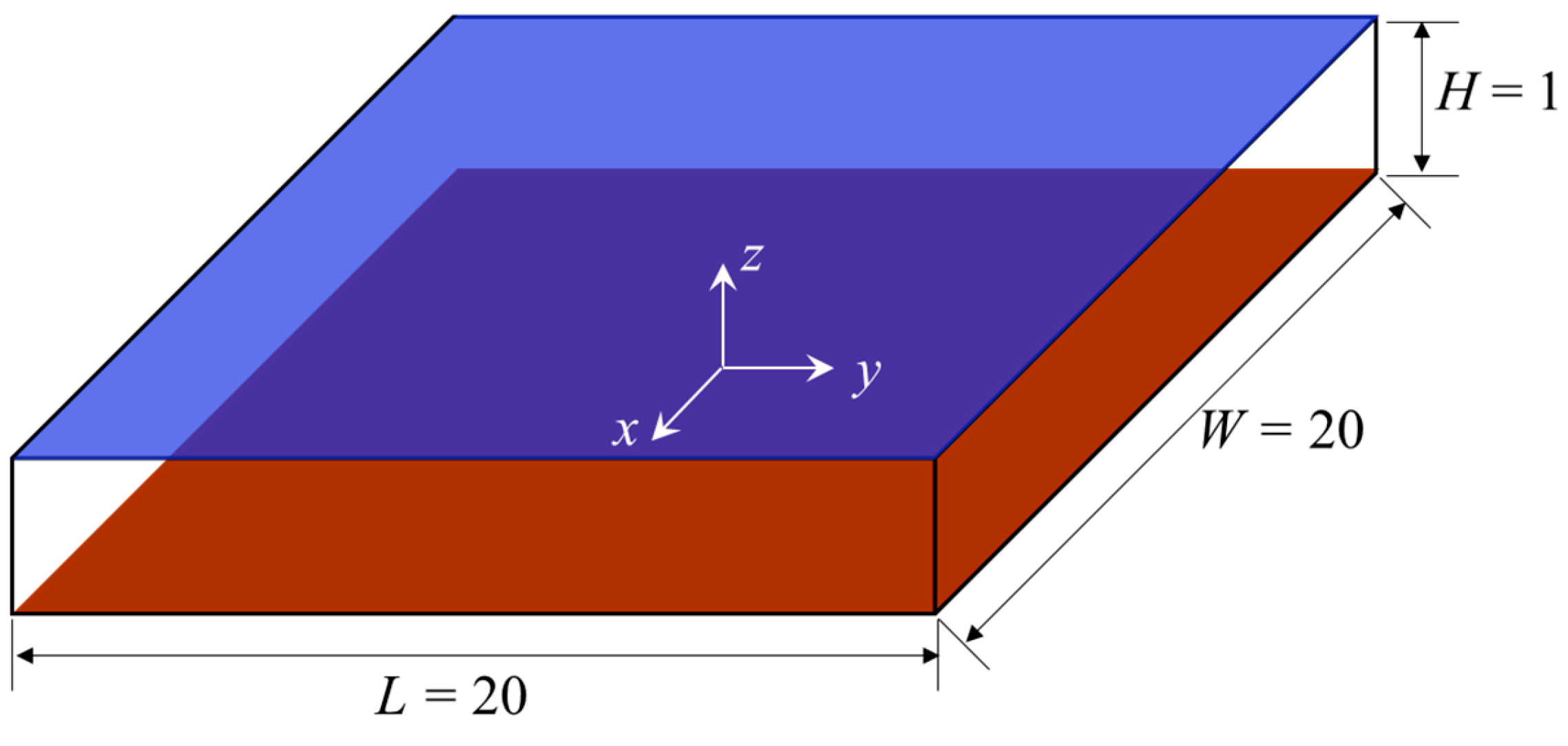
2.1. Basic Assumptions and Governing Equations

Under consideration is Bénard–Marangoni convection in an open cavity filled with liquid metal at low Prandtl numbers (Pr < 1), as illustrated in Figure 1. The cavity is L in length, W in width, and H in height. The high ratios of L/H and W/H are set to be 20 to reduce the boundary effects. The top boundary is the liquid-gas surface, with the assumption of nondeformable, as in many previous studies. The top boundary is air-cooled, the bottom boundary of the cavity is isothermal heated, and the four side boundaries are adiabatic. Marangoni stress is applied to the top boundary, while all the other five boundaries are rigid, impermeable, and no-slip walls. To investigate pure Bénard–Marangoni convection, gravity is neglected in this study.

In this study, 3D numerical procedures are employed to solve the Navier–Stokes equations. The dimensional mass, momentum and energy conservation equations with assumptions of incompressible Newtonian fluid and no gravity (the driving force is the thermocapillary force on the surface [5,7,26]) can be written as [26],

$$\frac{\partial u*}{\partial x*}+\frac{\partial v*}{\partial y*}+\frac{\partial w*}{\partial z*}=0,$$

(1)

$$\frac{\partial u*}{\partial t*}+u*\frac{\partial u*}{\partial x*}+v*\frac{\partial u*}{\partial y*}+w*\frac{\partial u*}{\partial z*}=-\frac{1}{\rho }\frac{\partial p*}{\partial x*}+\nu \left(\frac{{\partial }^{2}u*}{\partial x{*}^2}+\frac{{\partial }^{2}u*}{\partial y{*}^2}+\frac{{\partial }^{2}u*}{\partial z{*}^2}\right),$$

(2)

$$\frac{\partial v*}{\partial t*}+u*\frac{\partial v*}{\partial x*}+v*\frac{\partial v*}{\partial y*}+w*\frac{\partial v*}{\partial z*}=-\frac{1}{\rho }\frac{\partial p*}{\partial y*}+\nu \left(\frac{{\partial }^{2}v*}{\partial x{*}^2}+\frac{{\partial }^{2}v*}{\partial y{*}^2}+\frac{{\partial }^{2}v*}{\partial z{*}^2}\right),$$

(3)

$$\frac{\partial w*}{\partial t*}+u*\frac{\partial w*}{\partial x*}+v*\frac{\partial w*}{\partial y*}+w*\frac{\partial w*}{\partial z*}=-\frac{1}{\rho }\frac{\partial p*}{\partial z*}+\nu \left(\frac{{\partial }^{2}w*}{\partial x{*}^2}+\frac{{\partial }^{2}w*}{\partial y{*}^2}+\frac{{\partial }^{2}w*}{\partial z{*}^2}\right),$$

(4)

$$\frac{\partial \theta }{\partial t*}+u*\frac{\partial \theta }{\partial x*}+v*\frac{\partial \theta }{\partial y*}+w*\frac{\partial \theta }{\partial z*}=\kappa \left(\frac{{\partial }^2\theta }{\partial x{*}^2}+\frac{{\partial }^2\theta }{\partial y{*}^2}+\frac{{\partial }^2\theta }{\partial z{*}^2}\right).$$

(5)

Here, x*, y*, and z* are the dimensional spatial Cartesian coordinates, u*, v*, and w* denote dimensional velocity components in the x*, y*, and z* directions, respectively, t* is dimensional time, p* is dimensional pressure, θ is dimensional temperature, ν, κ, and ρ are the kinematic viscosity, thermal diffusivity, and the density of the working fluid.

The dimensionless variables may be normalized based on [26,27,28]: (i) x, y, and z by H, (ii) u, v, and w by Maκ/H, (iii) t by H²/Maκ, (iv) ∂p/∂x, ∂p/∂y, and ∂p/∂z by ρMa²κ²/H³, and (v) T by (θ − θ_s)/(θ_b − θ_s), where u, v, and w denote dimensionless velocity components in the x, y, and z directions, respectively, x, y, and z are the dimensionless spatial Cartesian coordinates, t is dimensionless time, p is dimensionless pressure, and T is dimensionless temperature, θ_b and θ_s are the dimensional temperature of the heating bottom boundary and the top boundary. According to the spatial Cartesian coordinates in Figure 1, the top boundary is z = 1, the bottom boundary z = 0, the four sides are x = 10, y = 10, x = −10, y = −10, respectively. For incompressible Newtonian fluid, there are ρ (p, T) = const, ν (p, T) = const, where ν is the kinematic viscosity.

The corresponding 3D dimensionless mass, momentum and energy conservation equations can be written as [26],

$$\frac{\partial u}{\partial x}+\frac{\partial v}{\partial y}+\frac{\partial w}{\partial z}=0,$$

(6)

$$\frac{\partial u}{\partial t}+u\frac{\partial u}{\partial x}+v\frac{\partial u}{\partial y}+w\frac{\partial u}{\partial z}=-\frac{\partial p}{\partial x}+\frac{Pr}{Ma}\left(\frac{{\partial }^{2}u}{\partial x^2}+\frac{{\partial }^{2}u}{\partial y^2}+\frac{{\partial }^{2}u}{\partial z^2}\right),$$

(7)

$$\frac{\partial v}{\partial t}+u\frac{\partial v}{\partial x}+v\frac{\partial v}{\partial y}+w\frac{\partial v}{\partial z}=-\frac{\partial p}{\partial y}+\frac{Pr}{Ma}\left(\frac{{\partial }^{2}v}{\partial x^2}+\frac{{\partial }^{2}v}{\partial y^2}+\frac{{\partial }^{2}v}{\partial z^2}\right),$$

(8)

$$\frac{\partial w}{\partial t}+u\frac{\partial w}{\partial x}+v\frac{\partial w}{\partial y}+w\frac{\partial w}{\partial z}=-\frac{\partial p}{\partial z}+\frac{Pr}{Ma}\left(\frac{{\partial }^{2}w}{\partial x^2}+\frac{{\partial }^{2}w}{\partial y^2}+\frac{{\partial }^{2}w}{\partial z^2}\right),$$

(9)

$$\frac{\partial T}{\partial t}+u\frac{\partial T}{\partial x}+v\frac{\partial T}{\partial y}+w\frac{\partial T}{\partial z}=\frac{1}{Ma}\left(\frac{{\partial }^{2}T}{\partial x^2}+\frac{{\partial }^{2}T}{\partial y^2}+\frac{{\partial }^{2}T}{\partial z^2}\right),$$

(10)

by considering the dimensionless parameters of Ma and Pr obtained from dimensional analysis,

$$Ma=-\frac{\alpha \left({\theta }_b-{\theta }_s\right)H}{\rho \nu \kappa },$$

(11)

$$Pr=\frac{\nu }{\kappa },$$

(12)

where α is the temperature coefficient of surface tension. The governing parameters of the Biot number (Bi) and Nusselt number (Nu) of the heated boundary may be defined as

$$\mathit{Bi}=-\frac{\mathit{hH}}{\lambda },$$

(13)

$$Nu=\frac{1}{S}{\displaystyle \iint \left(wTMa-\frac{\partial T}{\partial z}\right)\mathrm{d}S},$$

(14)

where h, λ, and S denote surface heat transfer coefficient, thermal conductivity of working fluid, and dimensionless area of the bottom boundary, respectively. Thus, the temperature difference between the bottom and top boundaries may be expressed as [20]

$${\theta }_b-{\theta }_s=\frac{Bi\left({\theta }_b-{\theta }_0\right)}{Bi+1},$$

(15)

where θ₀ refers to the reference temperature, which is the temperature of cool air.

The top boundary is imposed by the thermocapillary stress in numerical simulation [27], thus, the boundary conditions may be expressed as

$$\begin{array}{l}u=v=w=0,\frac{\partial T}{\partial x}=0,\mathrm{at}x=10,x=-10,\\ u=v=w=0,\frac{\partial T}{\partial y}=0,\mathrm{at}y=10,y=-10,\\ \frac{\partial u}{\partial z}=\frac{\partial T}{\partial x}\mathrm{and}\frac{\partial v}{\partial z}=\frac{\partial T}{\partial y},w=0,\frac{\partial T}{\partial z}=Bi\left(T-T_0\right),\mathrm{at}z=1,\\ u=v=w=0,T=1,\mathrm{at}z=0.\end{array}$$

(16)

2.2. The Numerical Method

The finite-volume method was utilized to solve the governing Equations (6)–(10) with a SIMPLE scheme for the pressure–velocity coupling. The methods of spatial discretization are Green–Gauss node based for gradient, second-order central difference for pressure, QUICK for momentum, and second-order upwind for energy. The residuals of continuity and velocities are smaller than 0.001. In this study, numerical simulations with the above discretization algorithm were performed on the FLUENT software. Double precision is adopted to improve the calculation accuracy. Parallel computing with a default setting and shared memory on local machine are used since the total number is as high. This method has been successfully used to simulate both laminar and turbulent flow of the Marangoni, thermocapillary and natural convections in many previous studies, and the results have been compared with available experimental results, which agree well with numerical results [26,28,29]. Since there are no experimental results of the Bénard–Marangoni convection with liquids at Prandtl numbers lower than unity under microgravity, no further validation is made in this study.

The mesh was built by the ICEM program. Its total number is 4.95 × 10⁶, and the average size of mesh was about 1 × 10⁻⁵ m, which means a very fine mesh. The physical parameters used in the simulations are according to liquid metals. The range of Prandtl numbers is from 0.01 to 0.06, which correspond to molten silicon and Gallium-indium-tin alloy. To investigate the flow structure from conduction state to supercritical bifurcations, numerical simulation was performed for Ma from 5.0 × 10¹ to 4.0 × 10⁴. The surface heat transfer coefficient of the liquid-gas surface is set to be 10 W m⁻² K⁻¹ based on the assumption of natural convection cooling of the air. The fluid properties, Biot number on top surface, and the range of Marangoni number are listed in

Table 1. The parameters used in the numerical simulation.

Fluid	Prandtl Number	Biot Number	Marangoni Number
Silicon melt [30]	0.011	0.0008	From 5.0 × 101 to 4.0 × 104
Liquid metal [31,32]	0.029	0.0030	From 5.0 × 101 to 4.0 × 104
Liquid metal [31,32]	0.063	0.0030	From 5.0 × 101 to 4.0 × 104

.

3. Results and Discussion

When the bottom boundary of the liquid cavity is uniformly heated from below, the fluid motion depends strongly on the temperature difference between the bottom and the ambient temperature. For small Ma, the liquid metal in the cavity is conduction dominated and there is no convection. The isothermal surface is flat and parallel to the bottom boundary. When Ma increases, convection may occur, cells may appear on the surface, and the isothermal surface may curve. As Ma increases to a critical value, the convection becomes pronounced and strong, the cells become distinct, and the isothermal surface becomes more curved. As Ma increases further, supercritical convection occurs, the flow becomes stronger even chaotic, the pattern of cells becomes more complex, the size of cells decreases, and the isothermal surfaces become much more curved. Since the temperature and velocity fields for the cases with the same Ma but different Prandtl numbers are similar, the results for liquid metal with Pr = 0.029 are chosen to be presented.

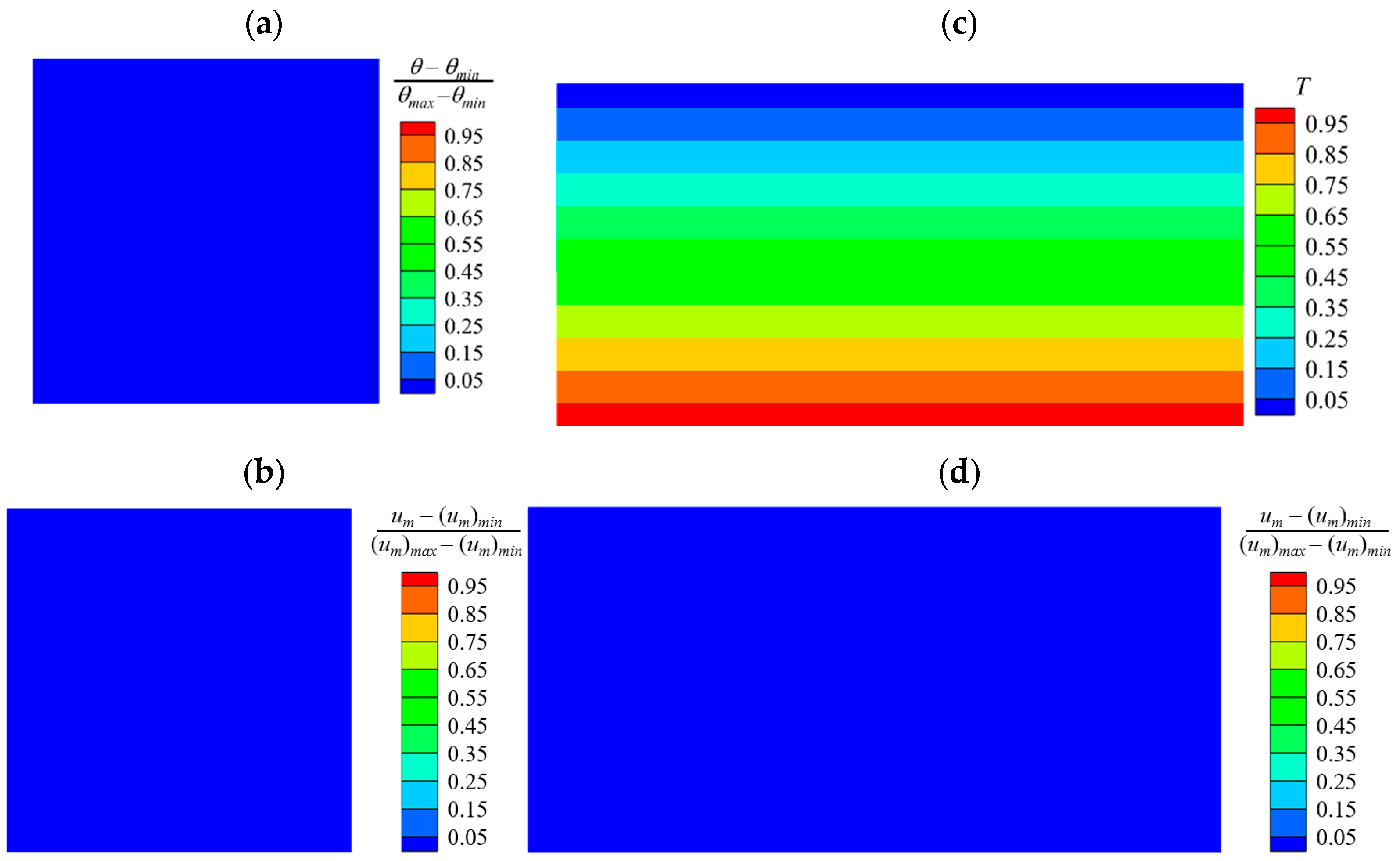
3.1. Conductive State

For the cases with Ma << Ma_c, the fluid layers with three different Prandtl numbers are dominated by conduction, and there is no convection. As illustrated in Figure 2, the isothermal surfaces are flat and parallel to the bottom boundary, the fluid is motionless, the top surface is isothermal at a temperature θ_s, which may be calculated by Equation (15). Note that for the better presentation of the temperature and velocity field at the slice of x = 0, the height of cavity is stretched. θ_max and θ_min denote the maximum and minimum temperature on the top surface, respectively. The velocity magnitude u_m is defined as (u² + v² + w²)^1/2. (u_m)_max and (u_m)_min denote the maximum and minimum velocity magnitude of the fluid in the cavity, respectively.

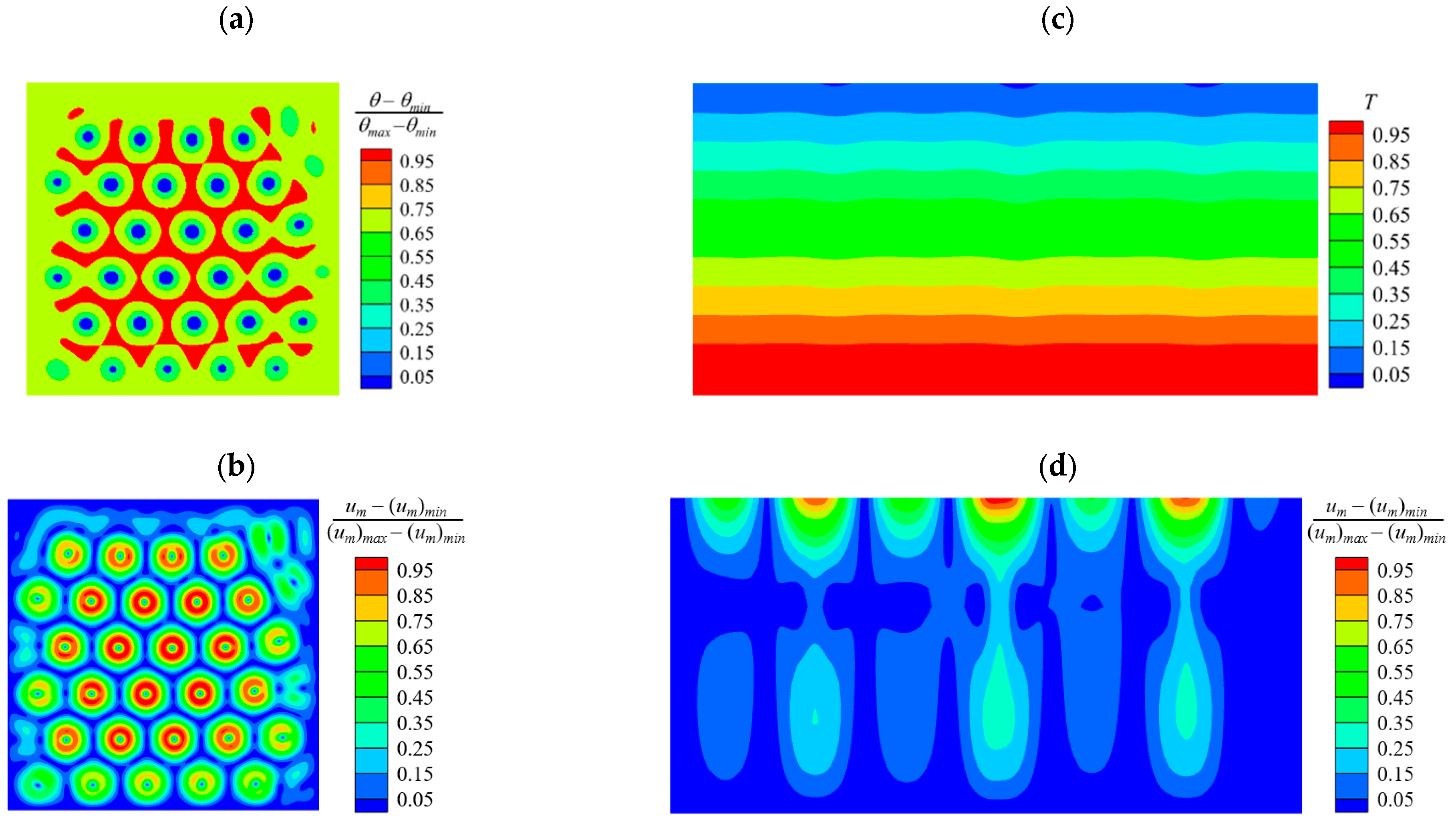
3.2. Critical Bifurcation

The critical Marangoni number predicted by previous work [6] is 79.6 under the condition of Bi = 0. In this work, the Biot numbers, which are close to zero, are listed in Table 1. Thus, the corresponding critical Marangoni number in this study may be 79.6. The temperature and velocity magnitudes for both surfaces and the x = 0 slice for the Ma = 80 cases are shown in Figure 3. As illustrated in Figure 3, symmetry breaking of the flow takes place, both the temperature and velocity field of the top surface show clear hexagonal cells except near the boundary of the cavity, which indicate the onset of Bénard–Marangoni convection as predicted by the previous study of critical bifurcation. It is worth noting that the centers of the cells are cold, but the outer regions are hot, and they are inversely proportional to the cells of the fluid at Prandtl numbers higher than unity. Such a phenomenon agrees with the theory of Rosenblat et al. [17,33] and the simulation result of Boeck and Thess, of which a periodic boundary condition is adopted rather than wall boundaries [20]. The isothermal surface is slightly bent due to convection. On the other hand, the isothermal surfaces at the slice of x = 0 are approximately parallel to the bottom boundary since the flow is weak. The average temperature on the top surface approximately equals to θ_s, which may be calculated by Equation (15).

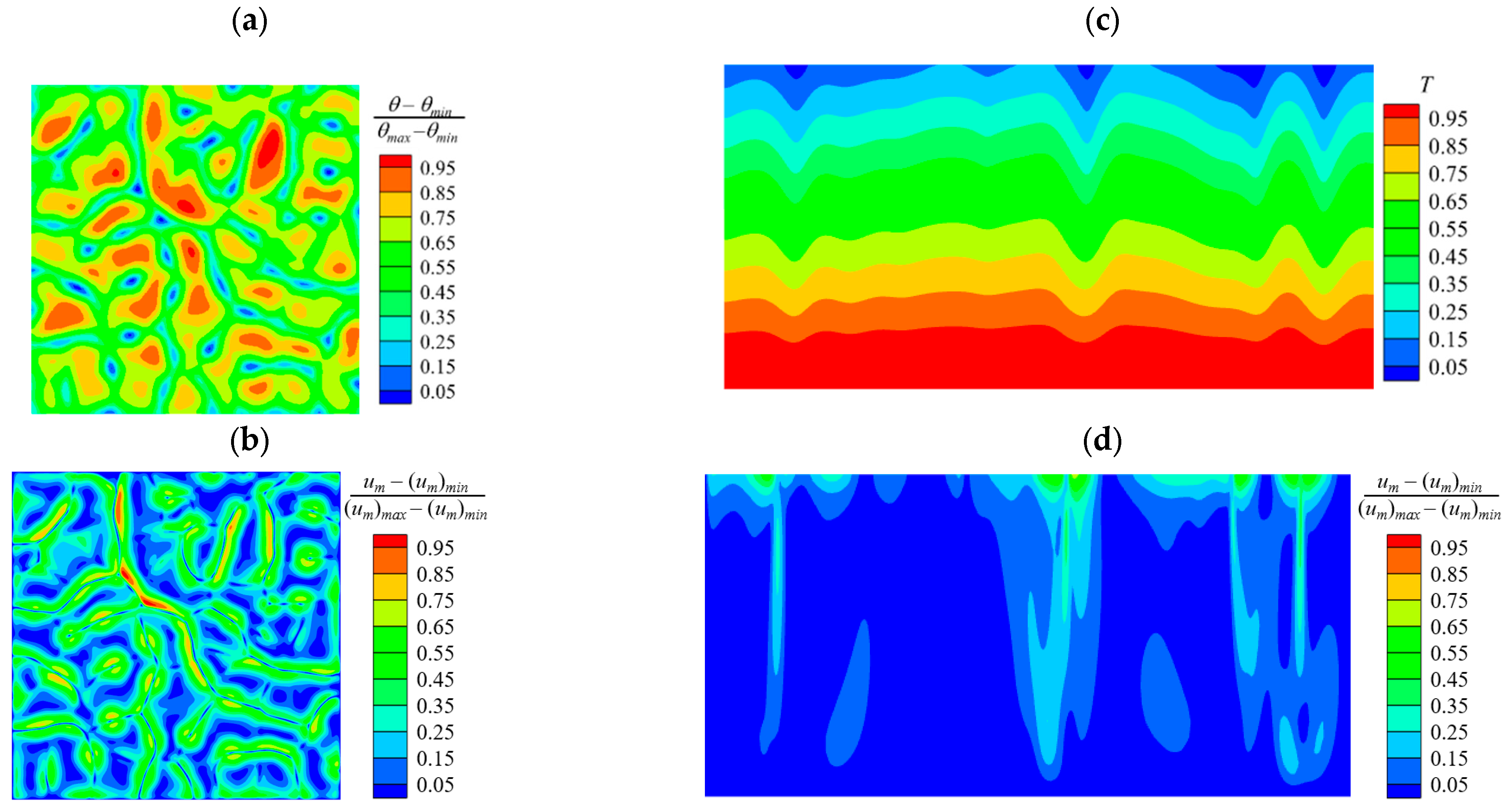
3.3. Supercritical Bifurcation

Increasing the Marangoni number further may lead to supercritical bifurcations. A dimensionless supercritical number may be defined as [34],

$$\epsilon =\frac{Ma-M{a}_c}{M{a}_c}.$$

(17)

Higher supercritical number of fluid layer indicates strong Bénard–Marangoni convection.

The numerical result for the case of ε = 0.25 is shown in Figure 4. Seen from Figure 4a,b, the symmetry of the flow is continuously broken, the temperature and velocity field on the top surface show irregular hexagonal cells. The centers of cells are cooler than the outer regions of cells. Seen from Figure 4c, the isothermal surfaces at the slice of x = 0 are inclined and curved, which means the convection is enhanced. This can be verified by the field of velocity magnitude at the slice of x = 0 in Figure 4d, of which the flow is stronger than that in the case with Ma = 80 in Figure 3.

The numerical result for the case of ε = 1.5 is shown in Figure 5. Seen from Figure 5a,b, the temperature and velocity fields on the top surface show irregular cells. It is worth noting that the centers of cells are still cooler than the outer regions of cells. Seen from Figure 5c, the isothermal surfaces at the slice of x = 0 are more inclined and curved than those with ε = 0.25 in Figure 4c, which means the convection is enhanced. This can be verified by the field of velocity magnitude at the slice of x = 0, of which the flow is stronger than that in the case with ε = 0.25 in Figure 4d.

As the supercritical number is increased further, the convection of the fluid flow becomes much stronger, as shown by the numerical result for the case with ε = 36.5 and Pr = 0.029, which is presented in Figure 6. Seen from the temperature and velocity field on the top surface in Figure 6a,b, the cells are difficult to identify. The average size of surface structures is obviously smaller than those in the case with ε = 0.25 and 1.5. The thermal boundary layer at the slice of x = 0 is thinner, the peak number of isothermal lines at the slice of x = 0 in Figure 6c is higher, and the columns of velocity magnitude at the slice of x = 0 in Figure 6d are more than those in the case with ε = 0.25 and 1.5.

Further increasing the Marangoni number to a supercritical number ε = 499 induces a much stronger flow convection, as presented in Figure 7. Compared with the result of the case with ε = 36.5 in Figure 6, the structure of convection cells is finer, as may be seen in Figure 7a,b. The thermal boundary layer beside the heated bottom boundary is thinner, and the peak number of isothermal lines at the slice of x = 0 in Figure 7c is higher, indicating a higher efficient heat transfer. The columns of velocity magnitude at the slice of x = 0 in Figure 7d are more, which means a much stronger flow and higher efficient of mass transfer.

3.4. Heat and Mass Transfer

In order to characterize convection quantitatively, it may be possible to measure the area-weighted mean velocity magnitude at the top boundary to quantify convection. The velocity magnitudes for different Marangoni numbers and Prandtl numbers are plotted in Figure 8.

A scaling of velocity magnitude may be obtained as,

$$u_m~MaP{r}^{-2/3},$$

(18)

which means the mass transfer may be enhanced by high Marangoni numbers and low Prandtl numbers.

To characterize the heat transfer quantitatively, the Nusselt number of the bottom boundary may be measured to quantify the heat transfer. The Nusselt numbers for different Marangoni numbers and Prandtl numbers are plotted in Figure 9. It is clear that Nu keeps almost constant value for Ma ≤ 400 but increases slowly for Ma > 400, which means the heat transfer is enhanced by the Bénard–Marangoni convection. In the range of 0 < Ma ≤ 4 × 10⁴, Nu~1 for all the three Prandtl numbers, but may increase fast with further increasing of Ma according to Boeck’s work [19].

4. Conclusions

In this study, 3D direct numerical simulations were performed to further understand the Bénard–Marangoni convection in an open cavity. The working fluids are liquids of silicon melt and liquid metals at Prandtl numbers lower than unity. Flow structures are presented and discussed for Prandtl numbers of 0.011, 0.029, and 0.063 and a wide range of Ma from 5.0 × 10¹ to 4.0 × 10⁴.

• For small Ma, the liquid metal in the cavity is conduction by conduction, and there is no convection.
• For Ma~Ma_c, the symmetry of flow is broken down, Bénard–Marangoni convection occurs and the hexagonal cells may be found on the surface. The critical Marangoni number agrees with that of fluids at Pr > 1. In the hexagonal cells in this study, the centers of the cells are cooler than the outer regions, which are different with the cells of fluid at Pr > 1. This phenomenon agrees with the prediction of Rosenblat [17].
• For Ma >> Ma_c, supercritical bifurcations may occur and are described by a supercritical number as Ma increases further. When the supercritical number is increased, the pattern of cells losses symmetry and becomes complex, the sizes of cells on the top surface decrease. Seen from the flow in the middle slice of the fluid at x = 0, the higher the supercritical number is, the thinner thermal boundary layers are, and the more intensive of the velocity columns are, indicating a stronger convection with higher Marangoni number.
• Heat and mass transfer in the transition route are quantified. The area-weighted mean velocity magnitude at the top boundary follows a scaling of u_m~Ma Pr^−2/3, which is a new scaling, which means the mass transfer may be enhanced by high Marangoni numbers and low Prandtl numbers. The Nusselt number is approximately constant for Ma ≤ 400 but increases slowly for Ma > 400, indicating that the heat transfer may be enhanced by increasing the Marangoni number.

This study investigates the Bénard–Marangoni convection in an open cavity filled with liquid metal, of which the Prandtl number is lower than 1. A series of the bifurcations are revealed, the temperature and velocity fields of convection are uncovered, heat and mass transfer in the cavity are quantified for a better understanding of the Bénard–Marangoni convection, and a new scaling of u_m~Ma Pr^−2/3 is found compared to previous studies. In the future, large-scale numerical simulations will be conducted to reveal the transition route to chaos for Bénard–Marangoni convection with liquid metal. Moreover, experiments can be carried out to explore the transient flow and compared to the numerical results. These investigations will further advance the understanding of Bénard–Marangoni convection and provide insights into applications of, e.g., material fabrication, crystal growth, chemical processes and welding.

References

1. Chen, S.; Zhang, Z.; Zhang, Y.; Sha, Y. A three-dimensional multiphase numerical model for the influence of Marangoni convection on Marangoni self-driven object. Phys. Fluids 2022, 34, 043308. [Google Scholar] [CrossRef]
2. Wissink, J.G.; Herlina, H. Surface-temperature-induced Marangoni effects on developing buoyancy-driven flow. J. Fluid Mech. 2023, 962, A23. [Google Scholar] [CrossRef]
3. Wang, H.; Liu, D.; Zheng, C.; Zhao, J.; Chang, J.; Hu, L.; Liao, H.; Geng, D.; Xie, W.; Wei, B. Spiral eutectic growth dynamics facilitated by space Marangoni convection and liquid surface wave. Phys. Fluids 2024, 36, 047137. [Google Scholar] [CrossRef]
4. Bénard, H. Les tourbillons cellulaires dans une nappe liquide. Rev. Gén. Sci. Pures Appl. 1900, 11, 1261–1271, 1309–1328. [Google Scholar]
5. Block, M.J. Surface tension as the cause of Bénard cells and surface deformation in a liquid film. Nature 1956, 178, 650–651. [Google Scholar] [CrossRef]
6. Pearson, J.R.A. On convection cells induced by surface tension. J. Fluid Mech. 1958, 4, 489–500. [Google Scholar] [CrossRef]
7. Nield, D.A. Surface tension and buoyancy effects in cellular convection. J. Fluid Mech. 1964, 19, 341–352. [Google Scholar] [CrossRef]
8. Scriven, L.E.; Sternling, C.V. On cellular convection driven by surface-tension gradients: Effects of mean surface tension and surface viscosity. J. Fluid Mech. 1964, 19, 321–340. [Google Scholar] [CrossRef]
9. Zhao, Y.; Wu, D.; Duan, L.; Wang, J.; Li, J.; Duan, L.; Kang, Q. Turbulence structure of the Rayleigh–Bénard convection using liquid CO2 as working fluid. Phys. Fluids 2024, 36, 015132. [Google Scholar] [CrossRef]
10. Wu, D.; Duan, L.; Kang, Q. Defects of Bénard cell on a propagating front. Phys. Fluids 2020, 32, 024107. [Google Scholar] [CrossRef]
11. Jeyabalan, S.R.; Chertovskih, R.; Gama, S.; Zheligovsky, V. Nonlinear Large-Scale Perturbations of Steady Thermal Convective Dynamo Regimes in a Plane Layer of Electrically Conducting Fluid Rotating about the Vertical Axis. Mathematics 2022, 10, 2957. [Google Scholar] [CrossRef]
12. Ma, X.; Huang, Y.; Huang, Y.; Liu, Z.; Li, Z.; Floryan, J.M. Experiments on Marangoni spreading–evidence of a new type of interfacial instability. J. Fluid Mech. 2023, 958, A33. [Google Scholar] [CrossRef]
13. Koschmieder, E.L.; Biggerstaff, M.I. Onset of surface-tension-driven Bénard convection. J. Fluid Mech. 1986, 167, 49–64. [Google Scholar] [CrossRef]
14. Schatz, M.F.; VanHook, S.J.; McCormick, W.D.; Swift, J.B.; Swinney, H.L. Onset of Surface-Tension-Driven Bénard Convection. Phys. Rev. Lett. 1995, 75, 1938–1941. [Google Scholar] [CrossRef] [PubMed]
15. Nitschke, K.; Thess, A. Secondary instability in surface-tension-driven Bénard convection. Phys. Rev. E 1995, 52, R5772–R5775. [Google Scholar] [CrossRef] [PubMed]
16. Koschmieder, E.L.; Switzer, D.W. The wavenumbers of supercritical surface-tension-driven Bénard convection. J. Fluid Mech. 1992, 240, 533–548. [Google Scholar] [CrossRef]
17. Rosenblat, S.; Davis, S.H.; Homsy, G.M. Nonlinear Marangoni convection in bounded layers. Part 1. Circular cylindrical containers. J. Fluid Mech. 1982, 120, 91–122. [Google Scholar] [CrossRef]
18. Ginde, R.M.; Gill, W.N.; Verhoeven, J.D. An experimental study of Reyleigh-Benard convection in liquid Tin. Chem. Eng. Commun. 1989, 82, 223–228. [Google Scholar] [CrossRef]
19. Boeck, T.; Thess, A. Turbulent Bénard-Marangoni Convection: Results of Two-Dimensional Simulations. Phys. Rev. Lett. 1998, 80, 1216–1219. [Google Scholar] [CrossRef]
20. Boeck, T.; Thess, A. Bénard–Marangoni convection at low Prandtl number. J. Fluid Mech. 1999, 399, 251–275. [Google Scholar] [CrossRef]
21. Boeck, T. Bénard–Marangoni convection at large Marangoni numbers: Results of numerical simulations. Adv. Space Res. 2005, 36, 4–10. [Google Scholar] [CrossRef]
22. Boeck, T.; Thess, A. Inertial Bénard–Marangoni convection. J. Fluid Mech. 1997, 350, 149–175. [Google Scholar] [CrossRef]
23. Awwad, F.A.; Ismail, E.A.A.; Gul, T. Heat and Mass Transfer Gravity Driven Fluid Flow over a Symmetrically-Vertical Plane through Neural Networks. Symmetry 2023, 15, 1288. [Google Scholar] [CrossRef]
24. Wang, S.; Niu, S.; Li, X.; He, G. An Experimental Study of the Effects of Asymmetric Pitching Motion on the Hydrodynamic Propulsion of a Flapping Fin. Symmetry 2024, 16, 302. [Google Scholar] [CrossRef]
25. Ye, Z.; Chen, Y.; Yang, C.; Wu, D.; Wang, J.; Hu, L.; Duan, L.; Kang, Q. The Mechanism of Droplet Thermocapillary Migration Coupled with Multi-Physical Fields. Symmetry 2023, 15, 2069. [Google Scholar] [CrossRef]
26. Chen, E.; Xu, F. Transient Marangoni convection induced by an isothermal sidewall of a rectangular liquid pool. J. Fluid Mech. 2021, 928, A6. [Google Scholar] [CrossRef]
27. Villers, D.; Platten, J.K. Influence of interfacial tension gradients on thermal convection in two superposed immiscible liquid layers. Appl. Sci. Res. 1990, 47, 177–191. [Google Scholar] [CrossRef]
28. Guo, Z.; Li, J.; Li, K.; Zhao, J.; Hu, W. Dependency of transition in thermocapillary convection on volume ratio in annular pools of large-Pr fluid in microgravity. Int. J. Heat Mass Transf. 2023, 208, 124059. [Google Scholar] [CrossRef]
29. Meng, X.; Chen, E.; Xu, F. Thermocapillary convection in a cuboid pool with a sidewall of different temperature sections. Int. Commun. Heat Mass Transf. 2024, 155, 107549. [Google Scholar] [CrossRef]
30. Li, Y.-R.; Imaishi, N.; Azami, T.; Hibiya, T. Three-dimensional oscillatory flow in a thin annular pool of silicon melt. J. Cryst. Growth 2004, 260, 28–42. [Google Scholar] [CrossRef]
31. Liu, T.; Sen, P.; Kim, C.-J. Characterization of nontoxic liquid-metal alloy Galinstan for applications in microdevices. J. Microelectromech. Syst. 2012, 21, 443–450. [Google Scholar] [CrossRef]
32. Gao, Y.; Wang, L.; Li, H.; Liu, J. Liquid metal as energy transportation medium or coolant under harsh environment with temperature below zero centigrade. Front. Energy 2013, 8, 49–61. [Google Scholar] [CrossRef]
33. Rosenblat, S.; Homsy, G.M.; Davis, S.H. Nonlinear Marangoni convection in bounded layers. Part 2. Rectangular cylindrical containers. J. Fluid Mech. 1982, 120, 123–138. [Google Scholar] [CrossRef]
34. Bragard, J.; Lebon, G. Non-Linear Marangoni Convection in a Layer of Finite Depth. Europhys. Lett. 1993, 21, 831. [Google Scholar] [CrossRef]
Figure 1. Schematic of physical model.
Symmetry 16 00844 g001
Figure 2. The temperature and velocity magnitude for cases with Ma << Mac. (a) The temperature field on the top surface. (b) The velocity magnitude on the top surface. (c) The temperature field at the slice of x = 0. (d) The velocity magnitude at the slice of x = 0. Note that the height of slice is stretched for better visualization.
Symmetry 16 00844 g002
Figure 3. The temperature and velocity magnitude for cases with Ma = 80 and Pr = 0.029. (a) The temperature field on the top surface. (b) The velocity magnitude on the top surface. (c) The temperature field at the slice of x = 0. (d) The velocity magnitude at the slice of x = 0. Note that the height of slice is stretched for better visualization.
Symmetry 16 00844 g003
Figure 4. The temperature and velocity magnitude for cases with ε = 0.25 and Pr = 0.029. (a) The temperature field on the top surface. (b) The velocity magnitude on the top surface. (c) The temperature field at the slice of x = 0. (d) The velocity magnitude at the slice of x = 0. Note that the height of slice is stretched for better visualization.
Symmetry 16 00844 g004
Figure 5. The temperature and velocity magnitude for cases with ε = 1.5 and Pr = 0.029. (a) The temperature field on the top surface. (b) The velocity magnitude on the top surface. (c) The temperature field at the slice of x = 0. (d) The velocity magnitude at the slice of x = 0. Note that the height of slice is stretched for better visualization.
Symmetry 16 00844 g005
Figure 6. The temperature and velocity magnitude for cases with ε = 36.5 and Pr = 0.029. (a) The temperature field on the top surface. (b) The velocity magnitude on the top surface. (c) The temperature field at the slice of x = 0. (d) The velocity magnitude at the slice of x = 0. Note that the height of slice is stretched for better visualization.
Symmetry 16 00844 g006
Figure 7. The temperature and velocity magnitude for cases with ε = 499 and Pr = 0.029. (a) The temperature field on the top surface. (b) The velocity magnitude on the top surface. (c) The temperature field at the slice of x = 0. (d) The velocity magnitude at the slice of x = 0. Note that the height of slice is stretched for better visualization.
Symmetry 16 00844 g007
Figure 8. The area-weighted average velocity magnitude of the top boundary.
Symmetry 16 00844 g008
Figure 9. The Nusselt number on the heated bottom boundary.
Symmetry 16 00844 g009