Symmetry-Optimized Dynamical Analysis of Optical Soliton Patterns in the Flexibly Supported Euler–Bernoulli Beam Equation: A Semi-Analytical Solution Approach

Abstract

This study employs spatial optimization principles to investigate the nonlinear vibration of a flexibly supported Euler–Bernoulli beam, a (1 + 1)-dimensional system subjected to axial loads. The modified Khater method, a crucial tool in mechanical engineering, is utilized to analyze analytical solutions, which include a symmetric spatial representation of the waveform as an integral part of each solution. Notably, periodic soliton solutions for the nonlinear model closely align with numerical and approximate analytical solutions, demonstrating the accuracy of our modeling approach. Density diagrams, contour diagrams, and Poincaré maps depicting the obtained analytical solutions are presented to elucidate their accuracy and provide visual confirmation of the optimized engineering model’s physical significance. The planar dynamical system is derived through the Galilean transformation by employing mathematical models and appropriate parameter values, thereby further refining problem understanding. Sensitivity analysis is conducted, and phase portraits with equilibrium points are illustrated by analyzing a special case of the investigated dynamical system, emphasizing its symmetrical properties. Lastly, we perform a global analysis to identify periodic, quasi-periodic, and chaotic behaviors, with an extra weak forcing term confirmed by Poincaré maps and a two-dimensional symmetric basin of the largest Lyapunov exponent.

1. Introduction

The demand for engineered construction is continually increasing. In structural engineering, the investigation of vibrations in beams is of great importance, especially in the context of tall structures, aerospace vehicles, large bridges, and various industrial applications. As the oscillation’s amplitude increases, these structures experience nonlinear vibrations, which can result in material fatigue and structural damage. The repercussions become more pronounced as the system approaches its inherent frequency. Consequently, precise mathematical and numerical analysis is imperative to comprehend the nonlinear vibration characteristics of these structures.

The design of such buildings necessitates careful consideration of multiple factors to optimize performance and extend their lifespan. Dynamic reactions of structures play a significant role in the design process. Distributed parameters and continuous systems, exemplified by the nonlinear vibration of beams, are addressed using linear and nonlinear partial differential equations (PDEs) in both spatial and temporal dimensions. Attaining precise or closed-form solutions for nonlinear issues has proven challenging.

Researchers have employed two primary categories of approximation solutions for initial boundary-value problems: numerical approaches [1,2] as well as approximate analytical approaches [3,4]. Perturbation methods have not been directly applied to solve nonlinear PDEs and their appropriate boundary conditions, especially in severely nonlinear systems. Consequently, the Galerkin method is employed to transform the initial partial differential equations into a set of nonlinear ordinary differential equations. Subsequently, these governing equations are analytically resolved in the time domain.

Numerous researchers have addressed the issue of vibrating beams by formulating partial differential equations of motion with diverse boundary conditions [5,6,7,8,9,10,11,12,13]. Bayat et al. [14] conducted an extensive investigation into the analytical evaluation of vibrating tapered beams, achieving notable progress in developing analytical solutions for nonlinear equations devoid of very small parameters. These advancements have been instrumental in approximating solutions for nonlinear oscillators.

Various classical methodologies, including perturbation techniques, have been employed to tackle the governing nonlinear differential equations for investigating nonlinear vibrations. Noteworthy methods include the Max-Min Approach [15], Homotopy Analysis Method [16,17], Iteration Perturbation Method [18], ADM-Padé technique [19], Homotopy Perturbation Method (HPM) [20], Adomian Decomposition [21], Energy Balance Method [22,23], Multistage Adomian Decomposition [24], Variational Iteration Method [25,26], Monotone Iteration Schemes [27], Hamiltonian Approach [28], Navier and Levy-type Solution [29,30], and Parameter Expansion Method [31].

A critical aspect of investigating nonlinear physical mechanisms involves exploring solutions in the form of traveling waves for nonlinear PDEs, which find applications in engineering sciences, mathematics, and technological fields. Nonlinear partial and ordinary differential equations (PDEs and ODEs) are crucial for simulating various significant phenomena in sciences such as mechanical engineering, biology, chemistry, and finance, as demonstrated in the literature [32,33,34,35].

Although numerous works exist on approximate analytical solutions in mechanical engineering, a gap persists in the literature regarding semi-analytical solutions. Therefore, this study aims to uncover soliton solutions with the aid of semi-analytical methods. The chosen methodologies encompass the $G^{\prime }/G$-expansion method [36], the Sardar sub-equation method [37], the modified simple equation method [38], the generalized Jacobi elliptic function method [39], the modified extended tanh scheme [40], the Kudryashov method [41], the improved Fan sub-equation method [42], the extended rational sine-cosine method [43], the unified method [44,45], the extended algebraic method [46], the new auxiliary equation technique [47], bifurcation analysis methods [48,49], and others.

According to Jhangeer et al. [50,51], the perturbed Fokas–Lenells equation has been demonstrated to have bifurcations, soliton structures, and chaotic dynamics. Solitons play a significant role in various physical phenomena and manifest in diverse forms, including kinks, light breathers, periodic structures, darkness, envelopes, and more. Imran et al. [52] show saddle-node bifurcation while studying the fractional space-time nonlinear Chen–Lee–Liu equation’s shift from periodic to quasi-periodic behavior. The work analyzes solitonic structures using direct algebraic methods and Galilean transformations to examine multi-dimensional bifurcations of dynamical solutions. A chaotic structure and multi-stability indicate a higher degree of complexity in the equation’s behavior.

In this investigation, we apply the Modified Khater Method (MKM)—a methodology not previously applied in the field of mechanical engineering of beams. Application of this effective technique to our experimental equation yields a visualization of novel wave patterns. Utilizing MKM, periodic soliton solutions, bright solutions, soliton-like solutions, mixed soliton solutions, and solitary bright solutions are attained. These results are expressed in terms of trigonometric and hyperbolic functions. The findings presented in this research have not been previously documented in the existing literature. The solutions developed in this study are new and hold significant utility across other scientific disciplines.

The Winkler model, introduced in 1867, incorporates the typical displacement of a structure. This model establishes a linear algebraic relationship between the normal displacement of the structure and the contact pressure [53]. Utilizing a set of mutually parallel and independent spring components to represent the soil medium, the Winkler model allows for a more straightforward comparison of the system’s nonlinear behavior compared to other approaches [54,55]. Wu and Liu [56] employed the technique of differential quadrature to address the buckling equation of a single-span Bernoulli-Euler beam. In 2006, they proposed the Parameterized-Perturbation method as a solution for highly nonlinear equations.

Osman and Omer [57] elucidated the relationship between curvature and bending moment in large-deformation Euler–Bernoulli beams, emphasizing distinctions between linear and nonlinear theories. Their work cautions against the indiscriminate use of nonlinear mathematical curvature, providing a numerical example for practical clarity. Pirbodaghi et al. [58] explored the nonlinear vibration characteristics of Euler–Bernoulli beams with geometric nonlinearity under axial loads using the homotopy analysis approach. They also examined the influence of vibration amplitude on nonlinear frequency and buckling load. In a study by Burgreen [59], the natural vibrations of a buckling beam supported at both ends were explored using a discretization method that considered a single mode of vibration. According to Burgreen, the buckling beam’s natural frequencies are vibration amplitude-dependent.

Abinash and Sundararajan [60] extend the Fragile Points Method (FPM) to analyze the behavior of isotropic and functionally graded Euler–Bernoulli beams under static bending, free vibration, and mechanical buckling. This is achieved through a meshless approach that utilizes discontinuous polynomial test and trial functions, along with numerical flux corrections, to enhance consistency. Pratiwi et al. [61] presents a Python-based tool that is validated against analytical solutions and commercial finite element solvers to efficiently and accurately analyze the structural response of wind turbine blades under aerodynamic loading using complex Euler–Bernoulli Beam theory and the polygon algorithm. Ataman and Szcześniak [62] analyze the dynamic response of a Bernoulli–Euler beam on a three-parameter inertial basis to moving forces. Deformable foundation properties, velocities, and foundation models all have an impact on beam dynamic deflection. The findings are a baseline for studying more complicated engineering structures under moving loads like road or railroad vehicles.

Upon examining the aforementioned achievements, the primary objective of this work is to derive the mathematical equation that describes the vibration behavior of clamped-clamped Euler–Bernoulli beams, considering their geometric nonlinearity. These beams are fixed at one end, and their geometric nonlinearity arises from the nonlinear interactions between strain and displacement, a topic frequently addressed in existing literature. This type of nonlinearity stems from various factors, including stretching in the middle of the structure, high curvatures in structural parts, and significant rotation of elements.

Initially, the governing nonlinear PDE was simplified to a solitary nonlinear ODE using the Galerkin technique under the assumption that only the basic mode was stimulated. Subsequently, this problem was analytically solved in the time domain using the MKM approach employed in this work. Finally, the results obtained from the proposed approach are compared with numerical solutions.

Finally, in relation to practical applications within the domain of engineering design and optimization, the precise semi-analytical solutions offered by the model can be utilized for the design and optimization of structures that involve Euler–Bernoulli beams. This application ensures enhanced reliability and performance, as demonstrated in studies such as [4,9,53].

Similarly, regarding vibration control and mitigation, gaining insight into the diverse, dynamic behaviors of beams can assist in formulating efficient vibration control and mitigation solutions. These solutions are essential for enhancing the durability and safety of engineering structures, as evidenced in [5,8,63,64,65,66].

The subsequent sections follow this sequence: Section 2 outlines the formulation of the problem. In Section 3, we illustrate the traveling wave solutions of the model under consideration. Section 4 presents the visualization and discussion of the dynamics of wave patterns, while Section 5.1 showcases phase portraits of the given planar dynamical system, incorporating bifurcation analysis. Moreover, Section 5.2 demonstrates the sensitivity of the system corresponding to initial conditions, and Section 5.3 depicts the chaotic behavior of the system with extra small harmonic forcing (perturbation) term, i.e., later verified with the help of Poincaré section and Lyapunov exponents spectra. Final conclusions drawn from these patterns are presented in Section 6.

2. Formulation of the Problem

A linear beam is supported by a flexible base and possesses properties such as length $\widehat{L}$, cross-sectional area $\widehat{A}$, mass per unit length $\widehat{\mu }$, moment of inertia $\widehat{I}$, and modulus of elasticity $\widehat{E}$. Additionally, the beam is subjected to an axial force of magnitude $\widehat{F}$ as shown in Figure 1. Assumptions include a uniform cross-sectional area and homogeneous material, in accordance with the Euler–Bernoulli beam theory. According to this theory, post-deformation, cross-sectional planes maintain their planar shape, while lines perpendicular to the central plane retain their perpendicularity. However, lines running across the cross-section do not change in length.

Three fundamental assumptions underpin the theory:

• Neglect of deformation within the same plane.
• Dismissal of transverse shear forces (resulting in cross-section rotation solely caused by bending).
• The incompressibility condition, which suggests the absence of transverse typical strains.

References supporting these assumptions include [65,67].

The equation of motion, considering the impact of mid-plane stretching, is expressed as follows:

$$\widehat{E}\widehat{I}\frac{{\partial }^4\widehat{W}}{\partial \widehat{X^4}}+\widehat{\mu }\frac{{\partial }^2\widehat{W}}{\partial {\widehat{t}}^2}+\widehat{F}\frac{{\partial }^2\widehat{W}}{\partial \widehat{X^2}}+\widehat{C}\frac{\partial \widehat{W}}{\partial \widehat{X}}+\widehat{K}\widehat{W}-\frac{\widehat{E}\widehat{A}}{2\widehat{L}}\frac{{\partial }^2\widehat{W}}{\partial \widehat{X^2}}{\int }_0^L{\left(\frac{\partial \widehat{W}}{\partial \widehat{X}}\right)}^{2}d\widehat{X}=V(\widehat{X},\widehat{t}).$$

(1)

The viscous damping coefficient is represented by $\widehat{C}$, the foundation modulus is denoted by $\widehat{K}$, and $\widehat{W}(\widehat{X},\widehat{t})$ is an unknown function, and V represents the distributed load in the transverse direction.

Let us assume that the non-conservative forces are negligible, meaning that the terms at $\widehat{C}$ and V are equal to zero. Therefore, Equation (1) can be expressed in the following manner:

$$\widehat{E}\widehat{I}\frac{{\partial }^4\widehat{W}}{\partial \widehat{X^4}}+\widehat{\mu }\frac{{\partial }^2\widehat{W}}{\partial {\widehat{t}}^2}+\widehat{F}\frac{{\partial }^2\widehat{W}}{\partial \widehat{X^2}}+\widehat{K}\widehat{W}-\frac{\widehat{E}\widehat{A}}{2\widehat{L}}\frac{{\partial }^2\widehat{W}}{\partial \widehat{X^2}}{\int }_0^L{\left(\frac{\partial \widehat{W}}{\partial \widehat{X}}\right)}^2\phantom{a}d\widehat{X}=0.$$

(2)

For enhanced convenience, we employ the following non-dimensional variables:

$$\overline{X}=\frac{\widehat{X}}{\widehat{L}},\phantom{aaa}\overline{W}=\frac{\widehat{W}}{\widehat{R}},\phantom{aaa}\overline{t}=\widehat{t}\sqrt{\frac{\widehat{E}\widehat{I}}{\widehat{\mu }\widehat{L^4}}},\phantom{aaa}\overline{F}=\frac{\widehat{F}\widehat{L^2}}{\widehat{E}\widehat{I}},\phantom{aaa}\overline{K}=\frac{\widehat{K}\widehat{L^4}}{\widehat{E}\widehat{I}}.$$

(3)

Here, the symbol $\widehat{R}$ represents the radius of gyration of the cross-section, which is calculated as $\widehat{R}=\sqrt{\widehat{I}/\widehat{A}}$. Therefore, Equation (2) yields:

$$\frac{{\partial }^4\overline{W}}{\partial \overline{X^4}}+\frac{{\partial }^2\overline{W}}{\partial \overline{t^2}}+\overline{F}\frac{{\partial }^2\overline{W}}{\partial \overline{X^2}}+\overline{K}\overline{W}-\frac{1}{2}\frac{{\partial }^2\overline{W}}{\partial \overline{X^2}}{\int }_0^L{\left(\frac{\partial \overline{W}}{\partial \overline{X}}\right)}^2\phantom{a}d\overline{X}=0.$$

(4)

By assuming that $\overline{W}(\overline{X},\overline{t})$ can be expressed as the product of $\delta \left(\overline{X}\right)$ and $\omega \left(\overline{t}\right)$, where $\delta \left(\overline{X}\right)$ represents the first eigenmode of the beam [66], and applying the Galerkin technique, we can derive the equation of motion as follows:

$${\ddot{\omega }}_{\left(\overline{t}\right)}+\alpha {\omega }_{\left(\overline{t}\right)}+\beta {\omega }_{\left(\overline{t}\right)}^3=0,$$

(5)

where $\alpha$ controls the linear stiffness, $\beta$ controls the amount of nonlinearity in the restoring force, $\alpha ={\alpha }_1+{\alpha }_2\overline{F}+\overline{K}$ and the values of ${\alpha }_1$, ${\alpha }_2$, and $\beta$ are as follows:

$${\alpha }_1=\frac{{\int }_0^1{\delta }^{iv}\delta dx}{{\int }_0^1{\delta }^{2}dx},\phantom{aaa}{\alpha }_2=\frac{{\int }_0^1{\delta }^{″}\delta dx}{{\int }_0^1{\delta }^{2}dx},\phantom{aaa}\beta =\frac{-0.5{\int }_0^1\left({\delta }^{″}{\int }_0^1{\delta }^{\prime 2}dx\right)\delta dx}{{\int }_0^1{\delta }^{2}dx}.$$

(6)

Equation (5) describes the governing nonlinear vibration behavior of Euler–Bernoulli beams. The equation is governed by the initial conditions specified at the center of the beam:

$${\omega }_{\left(0\right)}=A,{\dot{\omega }}_{\left(0\right)}=0,$$

(7)

where A stands for the dimensionless maximum amplitude of oscillation, the focus is on analyzing the natural response of the beam. This analysis starts with a specific displacement with no initial velocity, emphasizing the natural vibrational properties without any external or damping effects.

In this study, our initial attempt involved applying the Sardar sub-equation method to derive solutions for the equation. However, this approach proved unsuccessful, primarily due to square roots in the solution, hindering the separation of variables. Consequently, we turned to the modified Khater method, which proved to be a more suitable approach for addressing our problem.

3. The Traveling Wave Solutions

In this section, our focus is on finding the traveling wave solutions to Equation (1).

We generate wave patterns for the Euler–Bernoulli beam using the MKM based on Equation (5).

By employing the balancing strategy outlined in Appendix A, wherein we compare the highest-order linear and nonlinear terms, we determine the value of n. Specifically, we select the linear term ${\ddot{\omega }}_{\left(\overline{t}\right)}$, denoted as $n+2$, and the nonlinear term ${\omega }_{\left(\overline{t}\right)}^3$, denoted as $3n$, from Equation (5). Hence, we have $n+1=3n$. Solving this equation yields $n=1$, see [68] which we then substitute into Equation (A4). Thus, the resulting equation becomes:

$$V\left(\tau \right)={\lambda }_0+{\lambda }_1\Re \left(\tau \right),$$

(8)

where $\Re \left(\tau \right)$ is a solution of the ODE:

$$\dot{\Re }\left(\tau \right)=ln\left(v\right)({\sigma }_1+{\sigma }_2\Re \left(\tau \right)+{\sigma }_3{\Re }^2\left(\tau \right)).$$

(9)

By substituting Equations (8) and (9) into Equation (5) and performing simplifications, we derive a system of equations that provides the following set of solutions:

$$\begin{array}{cc}\hfill {\lambda }_0& ={\lambda }_0,{\lambda }_1=\frac{2{\lambda }_0{\sigma }_3}{{\sigma }_2}.\hfill \end{array}$$

(10)

The set of solutions for Equation (1) is obtained by using Equation (10):

• 1: If $\delta <0$ and ${\sigma }_3\ne 0$, then:

  $$\begin{array}{cc}\hfill {\overline{W}}_1(\overline{X},\overline{t})& =\frac{{\lambda }_0\sqrt{-\delta }}{{\sigma }_2}tan\left(\frac{\sqrt{-\delta }}{2}\tau \right),{\overline{W}}_2(\overline{X},\overline{t})=-\frac{{\lambda }_0\sqrt{-\delta }}{{\sigma }_2}cot\left(\frac{\sqrt{-\delta }}{2}\tau \right),\hfill \\ \hfill {\overline{W}}_3(\overline{X},\overline{t})& =\frac{{\lambda }_0\sqrt{-\delta }}{{\sigma }_2}\left(tan\left(\sqrt{-\delta }\tau \right)\pm \sqrt{mc}sec\left(\sqrt{-\delta }\tau \right)\right),\hfill \\ \hfill {\overline{W}}_4(\overline{X},\overline{t})& =-\frac{{\lambda }_0\sqrt{-\delta }}{{\sigma }_2}\left(cot\left(\sqrt{-\delta }\tau \right)\pm \sqrt{mc}csc\left(\sqrt{-\delta }\tau \right)\right),\hfill \\ \hfill {\overline{W}}_5(\overline{X},\overline{t})& =\frac{{\lambda }_0\sqrt{-\delta }}{2{\sigma }_2}\left(tan\left(\frac{\sqrt{-\delta }}{4}\tau \right)-cot\left(\frac{\sqrt{-\delta }}{4}\tau \right)\right).\hfill \end{array}$$

  (11)
• 2: If $\delta >0$ and ${\sigma }_3\ne 0$, then:

  $$\begin{array}{cc}\hfill {\overline{W}}_6(\overline{X},\overline{t})& =-\frac{{\lambda }_0\sqrt{\delta }}{{\sigma }_2}tanh\left(\frac{\sqrt{\delta }}{2}\tau \right),{\overline{W}}_7(\overline{X},\overline{t})=-\frac{{\lambda }_0\sqrt{\delta }}{{\sigma }_2}coth\left(\frac{\sqrt{\delta }}{2}\tau \right),\hfill \\ \hfill {\overline{W}}_8(\overline{X},\overline{t})& =-\frac{{\lambda }_0\sqrt{\delta }}{{\sigma }_2}\left(tanh\left(\sqrt{\delta }\tau \right)\pm \iota \sqrt{mc}sech\left(\sqrt{\delta }\tau \right)\right),\hfill \\ \hfill {\overline{W}}_9(\overline{X},\overline{t})& =-\frac{{\lambda }_0\sqrt{\delta }}{{\sigma }_2}\left(coth\left(\sqrt{\delta }\tau \right)\pm \sqrt{mc}csch\left(\sqrt{\delta }\tau \right)\right),\hfill \\ \hfill {\overline{W}}_{10}(\overline{X},\overline{t})& =-\frac{{\lambda }_0\sqrt{\delta }}{2{\sigma }_2}\left(tanh\left(\frac{\sqrt{\delta }}{4}\tau \right)+coth\left(\frac{\sqrt{\delta }}{4}\tau \right)\right).\hfill \end{array}$$

  (12)
• 3: If ${\sigma }_1{\sigma }_3>0$ and ${\sigma }_2=0$, then:

  $$\begin{array}{cc}\hfill {\overline{W}}_{11}(\overline{X},\overline{t})& =\frac{\left({\sigma }_2+2{\sigma }_3\left(\sqrt{\frac{{\sigma }_1}{{\sigma }_3}}tan\left(\sqrt{{\sigma }_1{\sigma }_3}\tau \right)\right)\right){\lambda }_0}{{\sigma }_2},\hfill \\ \hfill {\overline{W}}_{12}(\overline{X},\overline{t})& =\frac{\left({\sigma }_2-2{\sigma }_3\left(\sqrt{\frac{{\sigma }_1}{{\sigma }_3}}cot\left(\sqrt{{\sigma }_1{\sigma }_3}\tau \right)\right)\right){\lambda }_0}{{\sigma }_2},\hfill \\ \hfill {\overline{W}}_{13}(\overline{X},\overline{t})& =\frac{\left({\sigma }_2+2{\sigma }_3\left(\sqrt{\frac{{\sigma }_1}{{\sigma }_3}}\left(tan\left(2\sqrt{{\sigma }_1{\sigma }_3}\tau \right)\pm \sqrt{mc}sec\left(2\sqrt{{\sigma }_1{\sigma }_3}\tau \right)\right)\right)\right){\lambda }_0}{{\sigma }_2},\hfill \\ \hfill {\overline{W}}_{14}(\overline{X},\overline{t})& =\frac{\left({\sigma }_2+2{\sigma }_3\left(\sqrt{\frac{{\sigma }_1}{{\sigma }_3}}\left(-cot\left(2\sqrt{{\sigma }_1{\sigma }_3}\tau \right)\pm \sqrt{mc}csc\left(2\sqrt{{\sigma }_1{\sigma }_3}\tau \right)\right)\right)\right){\lambda }_0}{{\sigma }_2},\hfill \\ \hfill {\overline{W}}_{15}(\overline{X},\overline{t})& =\frac{\left({\sigma }_2+{\sigma }_3\left(\sqrt{\frac{{\sigma }_1}{{\sigma }_3}}\left(tan\left(\frac{\sqrt{{\sigma }_1{\sigma }_3}}{2}\tau \right)-cot\left(\frac{\sqrt{{\sigma }_1{\sigma }_3}}{2}\tau \right)\right)\right)\right){\lambda }_0}{{\sigma }_2}.\hfill \end{array}$$

  (13)
• 4: If ${\sigma }_1{\sigma }_3<0$ and ${\sigma }_2=0$, then:

  $$\begin{array}{cc}\hfill {\overline{W}}_{16}(\overline{X},\overline{t})& =\frac{\left({\sigma }_2-2{\sigma }_3\left(\sqrt{-\frac{{\sigma }_1}{{\sigma }_3}}tanh\left(\sqrt{-{\sigma }_1{\sigma }_3}\tau \right)\right)\right){\lambda }_0}{{\sigma }_2},\hfill \\ \hfill {\overline{W}}_{17}(\overline{X},\overline{t})& =\frac{\left({\sigma }_2-2{\sigma }_3\left(\sqrt{-\frac{{\sigma }_1}{{\sigma }_3}}coth\left(\sqrt{-{\sigma }_1{\sigma }_3}\tau \right)\right)\right){\lambda }_0}{{\sigma }_2},\hfill \\ \hfill {\overline{W}}_{18}(\overline{X},\overline{t})& =\frac{\left({\sigma }_2-2{\sigma }_3\left(\sqrt{-\frac{{\sigma }_1}{{\sigma }_3}}\left(tanh\left(2\sqrt{-{\sigma }_1{\sigma }_3}\tau \right)\pm \iota \sqrt{mc}sech\left(2\sqrt{-{\sigma }_1{\sigma }_3}\tau \right)\right)\right)\right){\lambda }_0}{{\sigma }_2},\hfill \\ \hfill {\overline{W}}_{19}(\overline{X},\overline{t})& =\frac{\left({\sigma }_2-2{\sigma }_3\left(\sqrt{-\frac{{\sigma }_1}{{\sigma }_3}}\left(coth\left(2\sqrt{-{\sigma }_1{\sigma }_3}\tau \right)\pm \sqrt{mc}csch\left(2\sqrt{-{\sigma }_1{\sigma }_3}\tau \right)\right)\right)\right){\lambda }_0}{{\sigma }_2},\hfill \\ \hfill {\overline{W}}_{20}(\overline{X},\overline{t})& =\frac{\left({\sigma }_2-{\sigma }_3\left(\sqrt{-\frac{{\sigma }_1}{{\sigma }_3}}\left(tanh\left(\frac{\sqrt{-{\sigma }_1{\sigma }_3}}{2}\tau \right)+coth\left(\frac{\sqrt{-{\sigma }_1{\sigma }_3}}{2}\tau \right)\right)\right)\right){\lambda }_0}{{\sigma }_2}.\hfill \end{array}$$

  (14)
• 5: If ${\sigma }_1={\sigma }_3$ and ${\sigma }_2=0$, then:

  $$\begin{array}{cc}\hfill {\overline{W}}_{21}(\overline{X},\overline{t})& =\frac{\left({\sigma }_2+2{\sigma }_3\left(tan\left({\sigma }_1\tau \right)\right)\right){\lambda }_0}{{\sigma }_2},{\overline{W}}_{22}(\overline{X},\overline{t})=\frac{\left({\sigma }_2-2{\sigma }_3\left(cot\left({\sigma }_1\tau \right)\right)\right){\lambda }_0}{{\sigma }_2},\hfill \\ \hfill {\overline{W}}_{23}(\overline{X},\overline{t})& =\frac{\left({\sigma }_2+2{\sigma }_3\left(tan\left(2{\sigma }_1\tau \right)\pm \sqrt{mc}sec\left(2{\sigma }_1\tau \right)\right)\right){\lambda }_0}{{\sigma }_2},\hfill \\ \hfill {\overline{W}}_{24}(\overline{X},\overline{t})& =\frac{\left({\sigma }_2+2{\sigma }_3\left(-cot\left(2{\sigma }_1\tau \right)\pm \sqrt{mc}csc\left(2{\sigma }_1\tau \right)\right)\right){\lambda }_0}{{\sigma }_2},\hfill \\ \hfill {\overline{W}}_{25}(\overline{X},\overline{t})& =\frac{\left({\sigma }_2+{\sigma }_3\left(tan\left(\frac{{\sigma }_1}{2}\tau \right)-cot\left(\frac{{\sigma }_1}{2}\tau \right)\right)\right){\lambda }_0}{{\sigma }_2}.\hfill \end{array}$$

  (15)
• 6: If ${\sigma }_1=-{\sigma }_3$ and ${\sigma }_2=0$, then:

  $$\begin{array}{cc}\hfill {\overline{W}}_{26}(\overline{X},\overline{t})& =\frac{\left({\sigma }_2-2{\sigma }_3\left(tanh\left({\sigma }_1\tau \right)\right)\right){\lambda }_0}{{\sigma }_2},{\widehat{W}}_{27}(\widehat{X},\widehat{t})=\frac{\left({\sigma }_2-2{\sigma }_3\left(coth\left({\sigma }_1\tau \right)\right)\right){\lambda }_0}{{\sigma }_2},\hfill \\ \hfill {\overline{W}}_{28}(\overline{X},\overline{t})& =\frac{\left({\sigma }_2+2{\sigma }_3\left(-tanh\left(2{\sigma }_1\tau \right)\pm \iota \sqrt{mc}sech\left(2{\sigma }_1\tau \right)\right)\right){\lambda }_0}{{\sigma }_2},\hfill \\ \hfill {\overline{W}}_{29}(\overline{X},\overline{t})& =\frac{\left({\sigma }_2+2{\sigma }_3\left(-coth\left(2{\sigma }_1\tau \right)\pm \sqrt{mc}csch\left(2{\sigma }_1\tau \right)\right)\right){\lambda }_0}{{\sigma }_2},\hfill \\ \hfill {\overline{W}}_{30}(\overline{X},\overline{t})& =\frac{\left({\sigma }_2-{\sigma }_3\left(tanh\left(\frac{{\sigma }_1}{2}\tau \right)+coth\left(\frac{{\sigma }_1}{2}\tau \right)\right)\right){\lambda }_0}{{\sigma }_2}.\hfill \end{array}$$

  (16)
• 7: If ${\sigma }_2^2=4{\sigma }_1{\sigma }_3$, then ${\overline{W}}_{31}(\overline{X},\overline{t})=\left(1-{\displaystyle \frac{4{\sigma }_1{\sigma }_3\left({\sigma }_2\tau ln\left(v\right)+2\right)}{{\sigma }_2^3\tau ln\left(v\right)}}\right){\lambda }_0.$
• 8: If ${\sigma }_2=\mu$, ${\sigma }_1=q\mu$$(q\ne 0)$, ${\sigma }_3=0$, then ${\overline{W}}_{32}(\overline{X},\overline{t})={\displaystyle \frac{\left({\sigma }_2+2{\sigma }_3\left(v^{\mu \tau }-q\right)\right){\lambda }_0}{{\sigma }_2}}.$
• 9: If ${\sigma }_2={\sigma }_3=0$, then ${\overline{W}}_{33}(\overline{X},\overline{t})={\displaystyle \frac{\left({\sigma }_2+2{\sigma }_3{\sigma }_1\tau ln\left(v\right)\right){\lambda }_0}{{\sigma }_2}}.$
• 10: If ${\sigma }_2={\sigma }_1=0$, then ${\overline{W}}_{34}(\overline{X},\overline{t})=\left(1-{\displaystyle \frac{2}{{\sigma }_2\tau ln\left(v\right)}}\right){\lambda }_0.$
• 11: If ${\sigma }_1=0$ and ${\sigma }_2\ne 0$, then

  $$\begin{array}{cc}\hfill {\overline{W}}_{35}(\overline{X},\overline{t})& =\left(1-\frac{2m}{cosh\left({\sigma }_2\tau \right)-sinh\left({\sigma }_2\tau \right)+m}\right){\lambda }_0,\hfill \\ \hfill {\overline{W}}_{36}(\overline{X},\overline{t})& =\left(1-\frac{2\left(cosh\left({\sigma }_2\tau \right)+sinh\left({\sigma }_2\tau \right)\right)}{cosh\left({\sigma }_2\tau \right)-sinh\left({\sigma }_2\tau \right)+c}\right){\lambda }_0.\hfill \end{array}$$

  (17)
• 12: If ${\sigma }_2=\mu$, ${\sigma }_3=q\mu$$(q\ne 0)$, ${\sigma }_1=0$, then

  $${\overline{W}}_{37}(\overline{X},\overline{t})=\left(1+\frac{2{\sigma }_{3}m{v}^{\mu \tau }}{\left(c-qm{v}^{\mu \tau }\right){\sigma }_2}\right){\lambda }_0.$$

  (18)

The presented approach marks the first application of solving the Euler–Bernoulli beam problem using a symmetric spatial representation of the waveform as part of each solution, which includes the $\tau$ function in ${\overline{W}}_i(\overline{X},\overline{t})$∀$i\in 1\dots 37$. Following the derivation of solutions, as detailed in Equation (10), their accuracy was validated by reintegrating them into the original Equation (5). Upon substitution, all solutions satisfied the equation, thus affirming their accuracy.

3.1. Strengths and Weaknesses

3.1.1. Strengths

• Direct method: Possibly producing quicker and more effective results, the modified Khater method looks for solutions directly rather than using iterative methods.
• Multiple exact solutions: It can often compute more than 1 exact solution to the same PDE. This gives you flexibility in how to analyze the behavior of your system and explore different scenarios.

3.1.2. Weaknesses

• Limited applicability: Not all nonlinear PDEs can be solved by the modified Khater approach. Especially complicated equations or ones with certain nonlinearities might not work well with it.
• Limited theoretical framework: The modified Khater approach may have a less developed theoretical framework than some well-known analytical techniques with a solid theoretical basis.

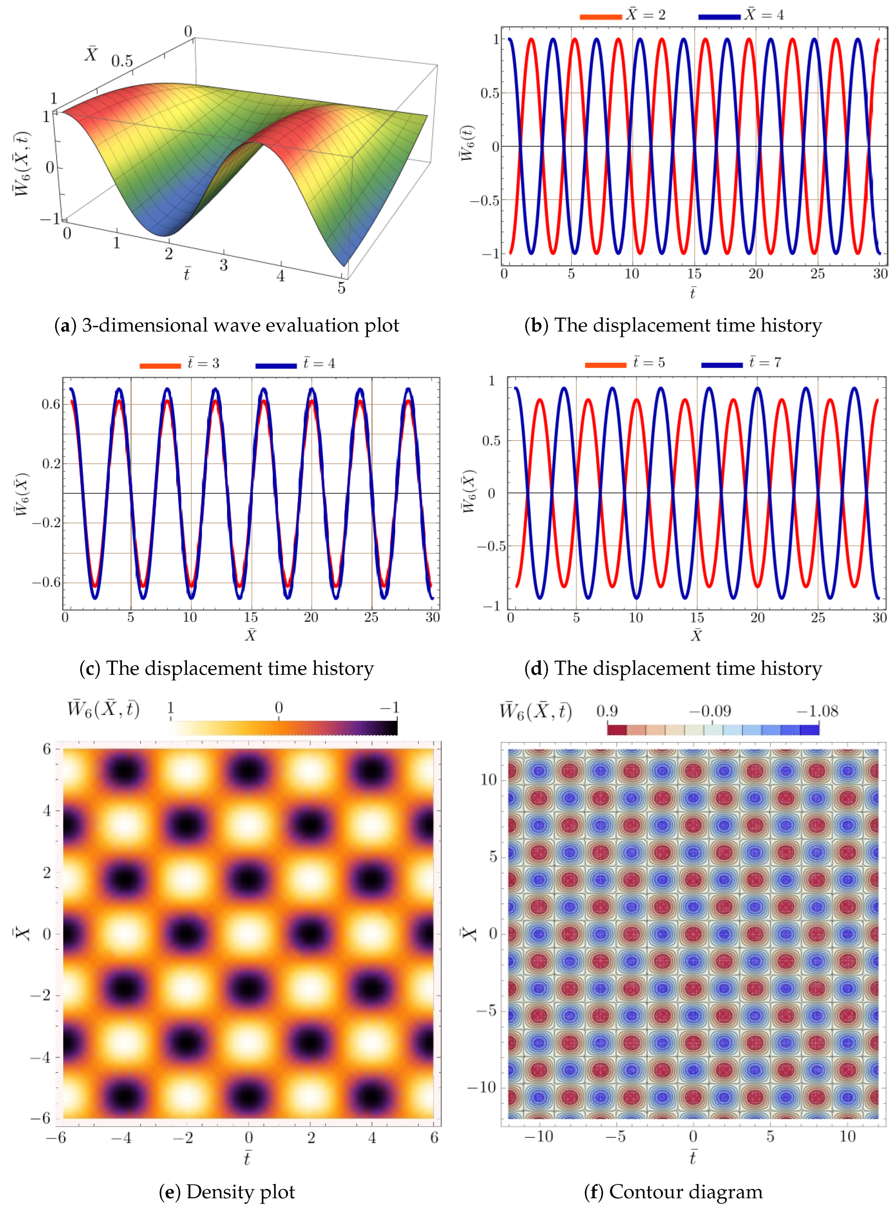
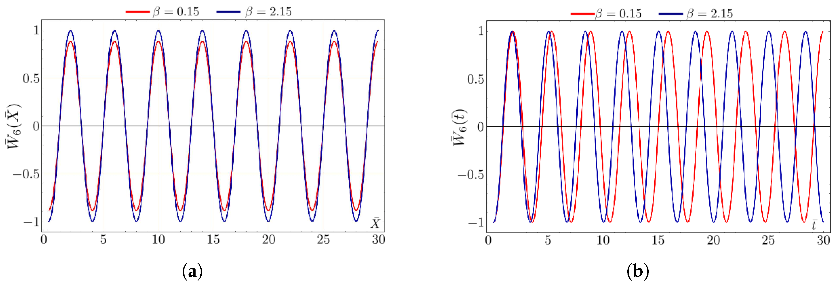
4. Visualization and Discussion of the Symmetric Wave Patterns

This study showcases the physical significance of the model through a representation of three- and two-dimensional density and contour diagrams, which illustrate the results obtained from numerical computations. These diagrams depict periodic soliton patterns, with each figure accompanied by a detailed list of model parameter values chosen carefully for accuracy.

In Figure 2 and Figure 3, we present a series of plots depicting the functions of selected solutions, ${\overline{W}}_6(\overline{x},\overline{t})$ and ${\overline{W}}_{37}(\overline{x},\overline{t})$, as described in Equations (12) and (18). Utilizing various types of plots allows us to illustrate the expected and correctly derived analytical solutions presented in the previous chapters. To assess the analytical solutions for the vibrations of the examined beam, density diagrams, and contour plots were employed to visualize and comprehend the behavior of this structure in time and space. The horizontal axis represents time $\overline{t}$, the vertical axis represents position $\overline{X}$, and density or contour levels represent the values of the deflection function $\overline{W}(\overline{x},\overline{t})$. These visual tools provide insights into several different aspects of the vibrations of the examined beam.

In Figure 2 and Figure 3e,f, the distribution of amplitude over time and space is illustrated. The values of the function $\overline{W}(\overline{x},\overline{t})$ are depicted using shades, revealing how the amplitude changes along the beam and over time as well. In Figure 3, we observe blurred and less distinct cyclically appearing regions compared to Figure 2. Additionally, under certain assumed boundary conditions and vibration frequencies, density diagrams revealed standing and traveling wave phenomena, where the deflection exhibits a characteristic pattern resembling a standing wave. Contour plots depict the dominant modes of vibration in the beam, with different contours corresponding to different vibration modes. As a result of this modal analysis, Figure 3 indicates a greater unevenness in the distribution of modes for the solution ${\overline{W}}_{37}(\overline{x},\overline{t})$.

Figure 4a,b illustrate the influence of the $\beta$ parameter on the dynamical response of ${\overline{W}}_6(\overline{X},\overline{t})$ at a specific time and position $\overline{X}$. In Figure 4a, it is evident that when time is held constant, the $\beta$ parameter affects the amplitude of the wave without inducing any phase difference. Conversely, in Figure 4b, the $\beta$ parameter does not impact the amplitude but causes a slight forward shift in the wave, resulting in a phase difference.

The fourth-order Runge–Kutta (RK4) numerical integration algorithm has been employed to numerically solve Equation (5). The obtained numerical solution serves as a means of comparison to validate our semi-analytical results and to demonstrate their closeness to the solutions derived from Equation (12), particularly ${\overline{W}}_6(\overline{X},\overline{t})$ as depicted in Figure 5. The approach involves discretizing the differential equation into small steps and iteratively calculating the approximate solution at each step.

Utilizing this precise and stable numerical method, we successfully captured the behavior of the system described by Equation (5). The numerical solutions exhibit satisfactory agreement with the semi-analytical solutions of the system ${\overline{W}}_6(\overline{X},\overline{t})$, confirming the reliability of our novel methodology in accurately depicting the dynamics of the system. This alignment between numerical and semi-analytical results highlights the strength of the numerical algorithm in approximating the mathematical model (5).

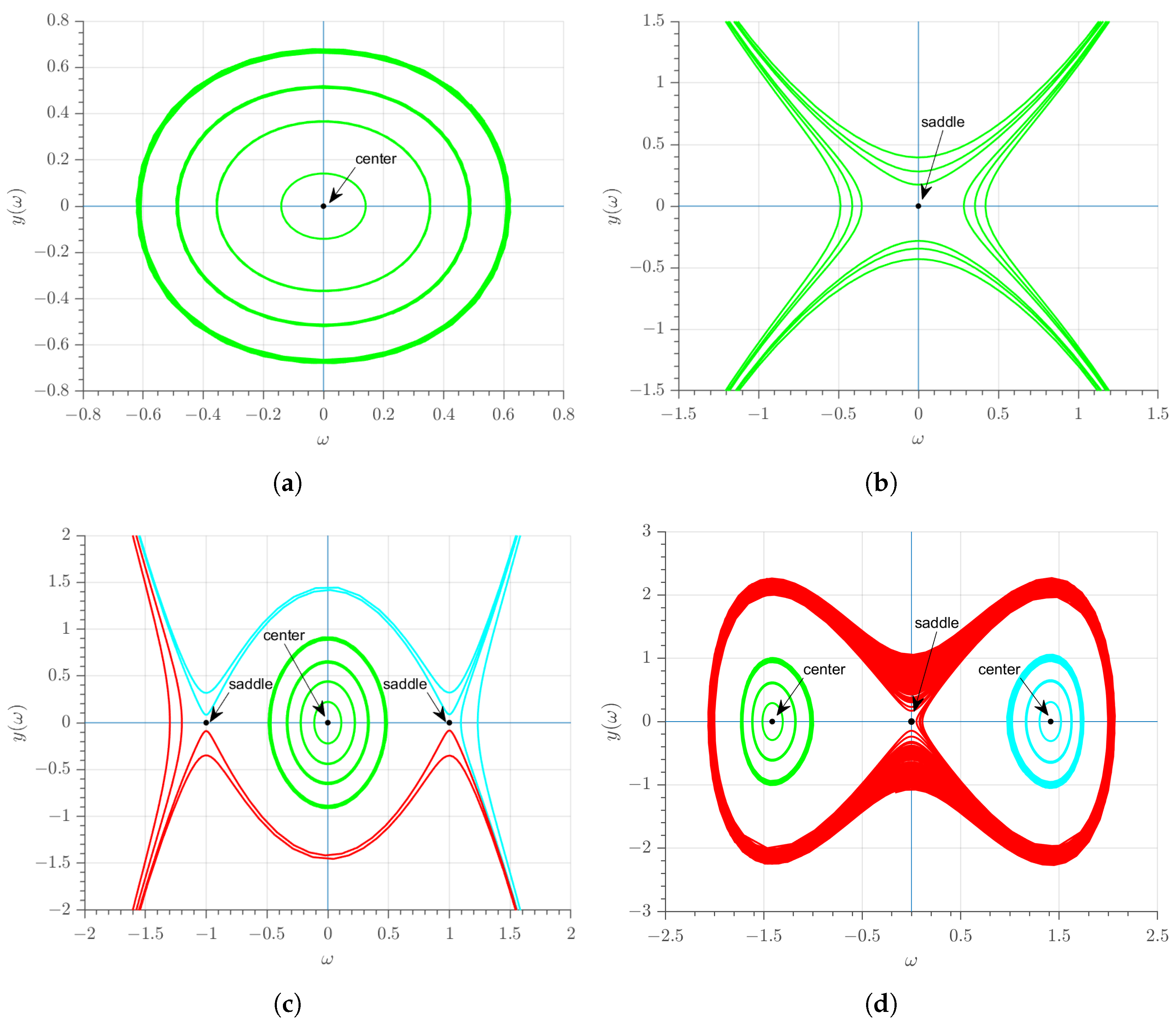
5. Dynamical Analysis

This section of the work explores the examined equation to unveil unexplored yet intriguing dynamics. The theories of sensitivity analysis, bifurcation, and chaos will be employed for this purpose. Given its applicability to a broad spectrum of independent variables, all subsequent calculations will be based on Equation (5).

5.1. Computation and Analysis of Equilibrium Points

After substituting $\dot{\omega }=y$ into Equation (5) and replacing $\widehat{t}$ with t, the resulting planar dynamical system is obtained:

$$\left\{\begin{array}{cc}{\displaystyle \frac{d\omega }{dt}}\hfill & =y\left(t\right),\hfill \\ {\displaystyle \frac{dy}{dt}}\hfill & =-\beta {\omega }^3\left(t\right)-\alpha \omega \left(t\right).\hfill \end{array}\right.$$

(19)

In relation to System (19), the first integral takes the form of a Hamiltonian

$$G(\omega ,y)=\frac{y^2}{2}+\frac{\beta }{4}{y}^4+\frac{\alpha }{2}{y}^2=H,$$

(20)

where H represents the Hamiltonian constant. The vector field of System (19) governs the phase orbits of this planar dynamical system.

Hence, it is important to examine various phase profiles of the System (19) using different parameters. The System (19) exhibits three equilibrium points for non-zero parameters $\alpha$ and $\beta$:

$$V_1=(0,0),V_2=\left(\sqrt{\frac{-\alpha }{\beta }},0\right),V_3=\left(-\sqrt{\frac{-\alpha }{\beta },0}\right).$$

(21)

The expression for the Jacobian of the linearized System (19) is given by

$$J(\omega ,y)=\left|\begin{array}{ccccc}0& & & & 1\\ -3\beta {\omega }^2-\alpha & & & & 0\end{array}\right|=3\beta {\omega }^2+\alpha .$$

(22)

The equilibrium points $(V_i,0)$, $i=1,2,3$ exhibit distinct characteristics determined by the value of $J(\omega ,y)$, as shown in Figure 6.

They act as saddle points when $J(\omega ,y)<0$, as centers when $J(\omega ,y)>0$, and as cuspidal points when $J(\omega ,y)=0$. To illustrate the phase portrait analysis of System (19), we explored various combinations of the parameters. The phase portraits illustrating the dynamical behavior of the system in Figure 6 depend on the following configurations of parameters:

• Case 1: $\alpha >0$ and $\beta >0$ Three equilibrium points are obtained from the System (19) by assigning specific values to the free parameters, such as $\alpha ,\beta =1$: $V_1=(0,0)$, $V_2=(\iota ,0)$, and $V_3=(-\iota ,0)$. The only actual point, denoted as $V_1$, is illustrated in Figure 6a, as $V_2$ and $V_3$ are imaginary.
• Case 2: $\alpha <0$ and $\beta <0$ Three equilibria are obtained from the System (19) with specific values assigned to $\alpha ,\beta =-1$: $V_1=(0,0)$, $V_2=(-\iota ,0)$, and $V_3=(\iota ,0)$. The only actual point $V_1$, is shown in Figure 6b, as $V_2$ and $V_3$ are imaginary.
• Case 3: $\alpha >0$ and $\beta <0$ Three equilibria are obtained from the System (19) by assigning $\alpha =1$ and $\beta =-1$: $V_1=(0,0)$, $V_2=(1,0)$, and $V_3=(-1,0)$. In this case, $V_2$ and $V_3$ indicate saddle points, while $V_1$ represents a center; see Figure 6c.
• Case 4: $\alpha <0$ and $\beta >0$ Three equilibria are obtained from the System (19) with specific values $\alpha =-2$ and $\beta =1$: $V_1=(0,0)$, $V_2=(1.4142,0)$, and $V_3=(-1.4142,0)$. In this case, $V_2$ and $V_3$ represent centers, while $V_1$ is a saddle point; see Figure 6d.

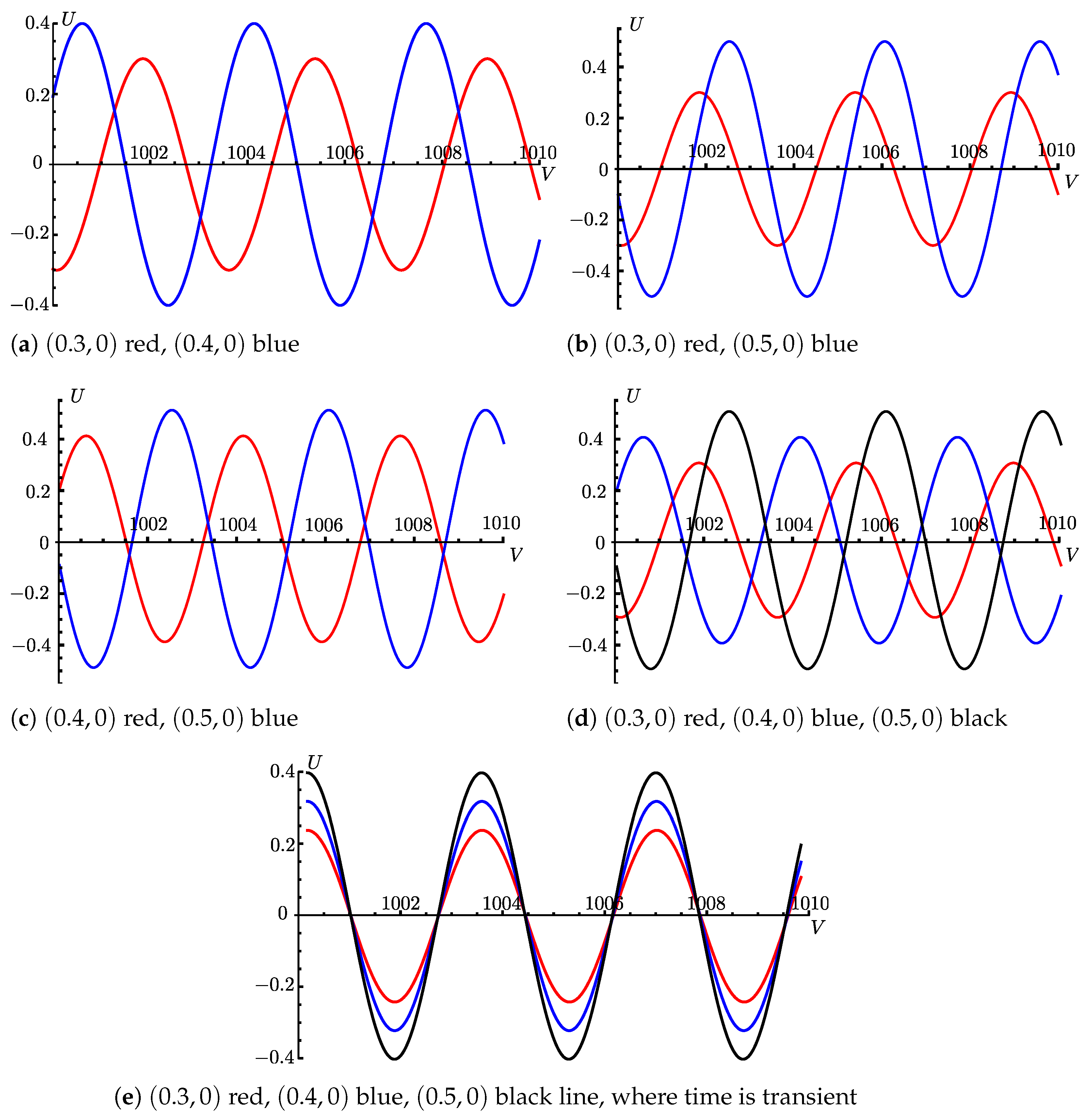
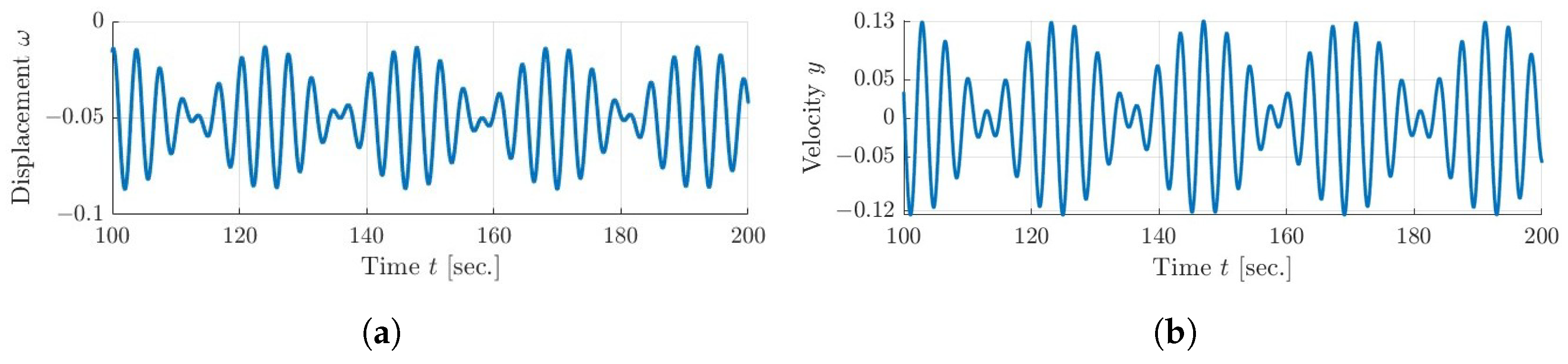
5.2. The Sensitivity Analysis

This section addresses the sensitivity analysis of the complex structure described by Equation (19) from an optimization perspective.

Figure 7a–d depicts three distinct configurations of initial conditions alongside several cases. Specifically, in Figure 7e, the red curve corresponds to $(U,V)=(0.3,0)$, the blue curve to $(U,V)=(0.4,0)$, and the black curve to $(U,V)=(0.5,0)$, indicating transient time. During this transient period, as illustrated in Figure 7e, the system demonstrates insensitivity. However, upon transitioning beyond the transient state, as evidenced in Figure 7a–c, System (19) exhibits a notably high level of sensitivity.

At the end, the comparison was conducted using various initial values, specifically $(0.3,0)$, $(0.4,0)$, and $(0.5,0)$, as illustrated in Figure 7d. The results clearly indicate that even minor variations in the initial values of System (19) significantly impact the final output. Consequently, it can be inferred that the investigated model is highly sensitive to initial conditions, lacking a transitional state.

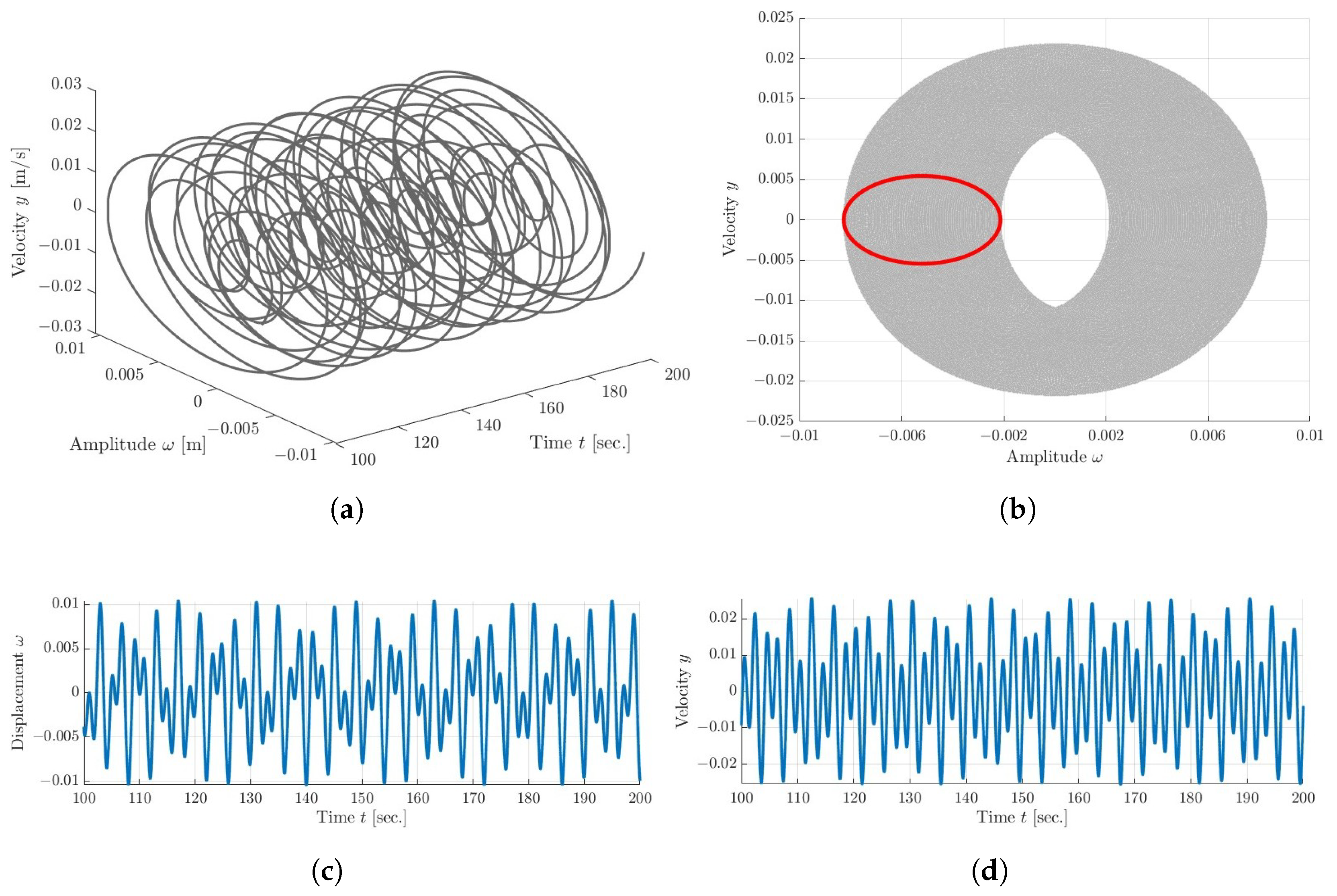
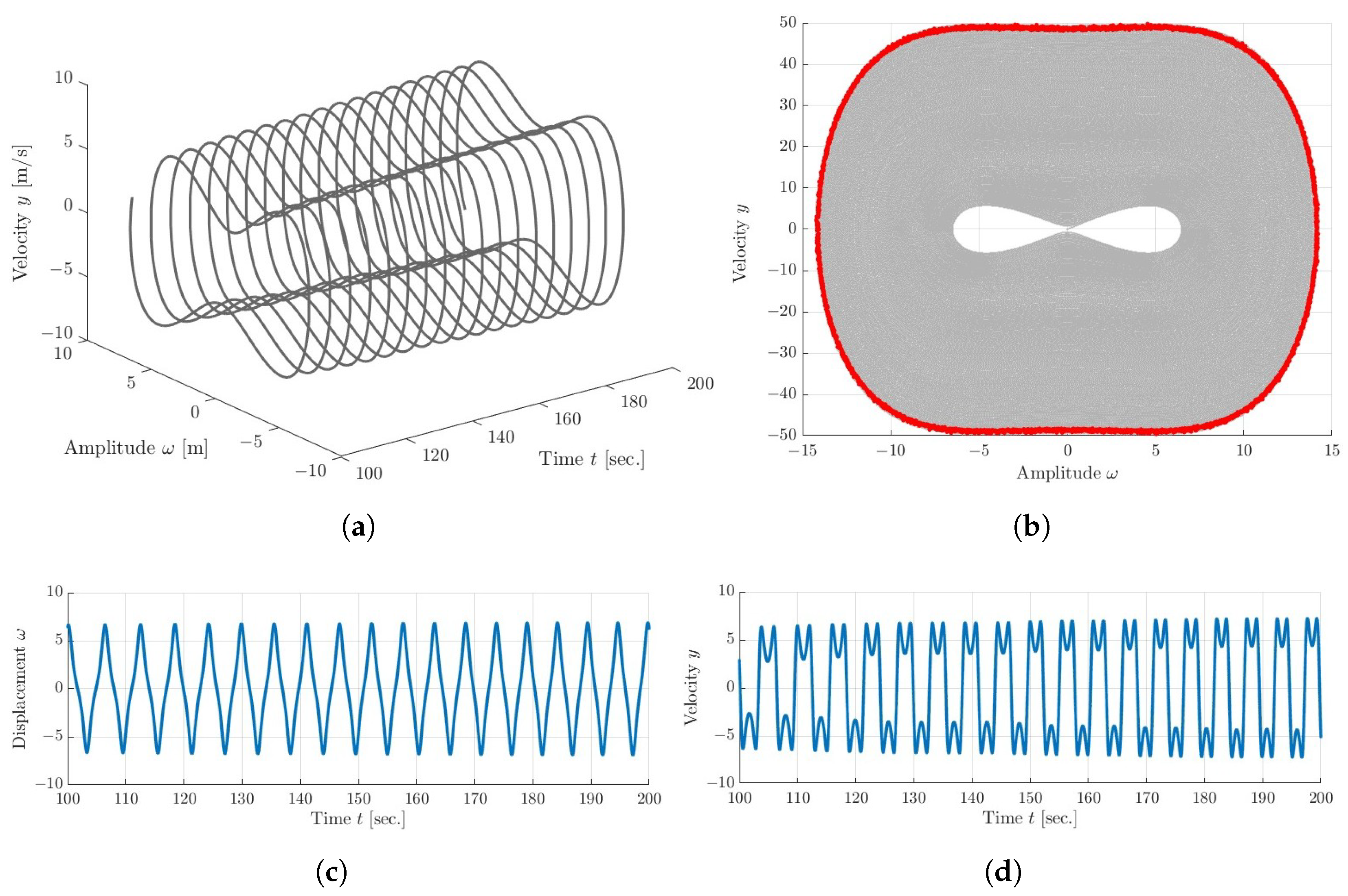
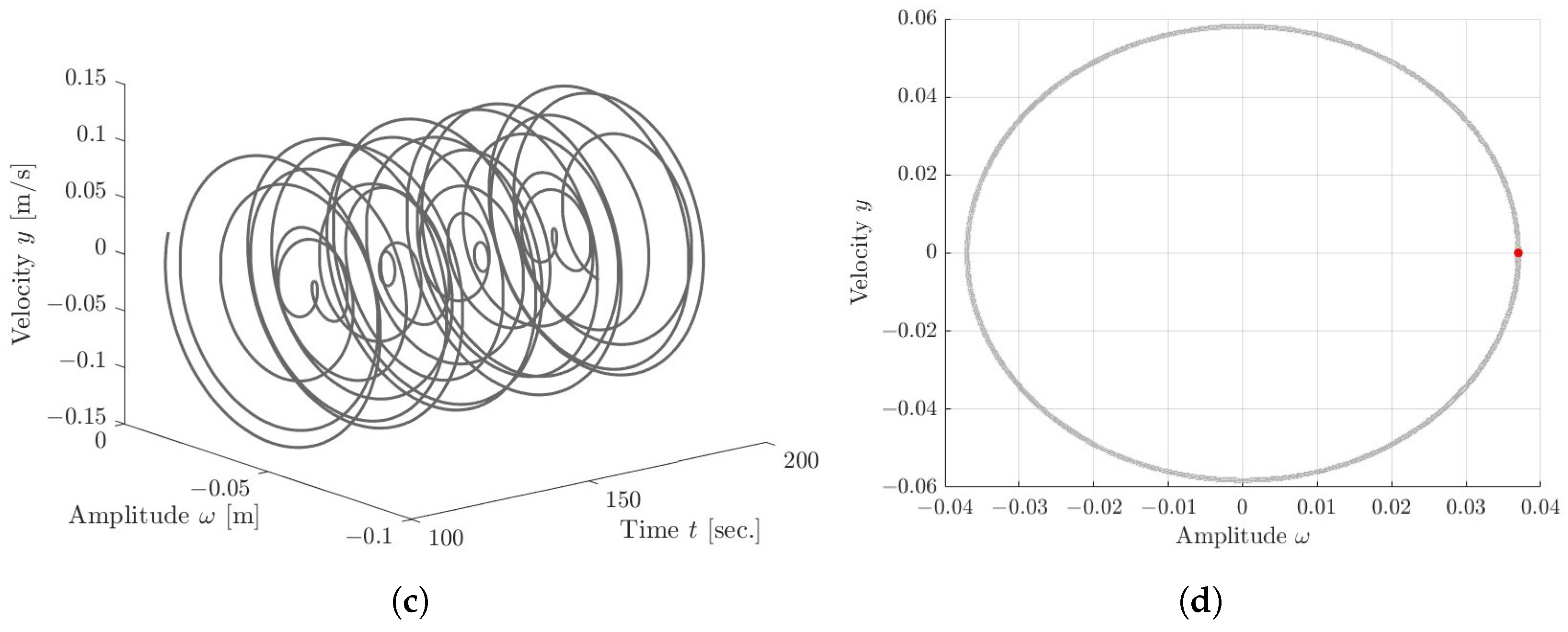
5.3. Quasi-Periodic and Chaotic Dynamics

The primary focus of this section is on describing the quasi-periodic, chaotic, and periodic dynamics governed by the 2-DOF ODE under investigation. Equation (19) is now supplemented with the weak forcing term $\epsilon cos\left(\vartheta t\right)$. Therefore, the following system may be expressed using Equation (19), including an extra forcing term (a form of perturbation):

$$\left\{\begin{array}{c}{\displaystyle \frac{d\omega }{dt}}=y,\hfill \\ {\displaystyle \frac{dy}{dt}}=-\beta {\omega }^3-\alpha \omega +\epsilon cos\left(\vartheta t\right),\hfill \end{array}\right.$$

(23)

where $\vartheta$ denotes the angular frequency and $\epsilon$ describes the small amplitude of the harmonic force. The introduction of the external periodic force, absent in System (19), is now incorporated into System (23). To explore the various dynamic effects covered by the description in Equation (1), a weak forcing term with parameters $\epsilon$ and $\vartheta =\pi$ is introduced while still considering the sustained influence of an external force with a certain excitation frequency, acting vertically at one end, and simultaneously taking into account specific physical properties of the model.

Figure 8, Figure 9 and Figure 10 depict quasi-periodic, chaotic, and periodic two-dimensional phase plane orbits versus time $t\in [100,200]$ s, respectively.

The dynamical responses shown in Figure 8 and Figure 9 are observed in the appropriate phase space and are obtained for the same set of model parameters, differing only in the signs of $\alpha$ and $\beta$. For instance, a time history spanning 20,000 s demonstrated in Figure 9 confirms a very weak dissipation of energy, resulting in a prolonged convergence time to the steady, albeit chaotic, dynamical state. In Figure 8, the periodic system response is found to be somewhat faster, as confirmed by the closed red Poincaré map, albeit with a quasi-periodic behavioral shift.

The dynamic responses, as illustrated in Figure 10, are observed in the corresponding phase plane for different sets of model parameters: $\alpha =3.41$, $\beta =2.15$, $\vartheta =\pi /2$, and a small amplitude of $\epsilon =0.035$. For example, the 60000-s time history depicted in Figure 10 confirms a prolonged convergence time to steady and periodic dynamics.

The dynamical system described by Equation (23) exhibits chaotic behavior under weak forcing, as depicted in Figure 9 for a steady-state irregular solution.

In addition to the Poincaré maps, the presence of quasi-periodic, chaotic, and periodic behavior is confirmed by the Lyapunov exponent spectra, presented in

Table 1. Lyapunov exponents spectra.

Figure	${\mathit{t}}_{\mathbf{end}}$	${\mathit{\lambda }}_{\mathbf{1}}$	${\mathit{\lambda }}_{\mathbf{2}}$
Figure 8	2000	0.000010	−0.000010
Figure 9	2000	0.170928	−0.170928
Figure 10	2000	0.000686	−0.000686

.

From the physics point of view, the influence of parameter $\alpha$ variation is illustrated in Figure 11a and the initial conditions imposed on the position and initial velocity on the dynamics of vibrations of the considered beam in Figure 11b. It is evident that both dependencies exhibit a symmetric nature of the physical system with respect to the zero velocity value, indicating a boundary of direction change. Within the range $\alpha =(-0.7;0.7)$, the motion may exhibit chaotic behavior, while outside of this range, it remains periodic, assuming that the remaining parameters of the model remain constant, with values of $\beta =2.15$, $\epsilon =0.035$, and $\theta =\pi /2$ (as depicted in the particular dynamic response in Figure 10). In this case, periodic motion was observed, confirming the significance of the special value of parameter $\alpha =3.41$, located outside the window $(-0.7;0.7)$ in which the dynamical response is mostly expected to be unstable.

Subsequently, we chose one of the values of parameter $\alpha$ and examined the sensitivity of the investigated dynamical system to changes in initial conditions, as visible in Figure 11b. A series of dark points symmetrically distributed on a yellow background can be observed. In these areas, the system will be more sensitive to changes in the pair of initial conditions $(\omega ,y)$, and in places of almost black color, where the largest Lyapunov exponent exceeds $0.01$, chaotic or quasi-periodic motion will occur. It is interesting to note that these areas consist of scattered points, yet the map maintains its symmetry.

6. Conclusions

In this study, the symmetry-optimized method of solution for a boundary- and initial-value problem, coupled with its dynamical analysis, enabled us to tackle two primary tasks. Firstly, we aimed to derive precise, explicit semi-analytical solutions. Secondly, we sought to analyze the dynamical behavior of the integrable Euler–Bernoulli beam model, representing a two-dimensional dynamical system subjected to axial load from one end and vertical forcing from the other. Employing the modified Khater approach allowed us to obtain precise, explicit solutions, including periodic soliton solutions presented in polynomials as well as rational function forms. The existence of these solutions was found to depend on the fulfillment of stable and favorable conditions, as illustrated through various graphical representations.

Furthermore, the phase portraits of the extracted two-degree-of-freedom dynamical system governing the nonlinear vibration behavior of the analyzed Euler–Bernoulli beams reveal planar orbits with equilibrium points of two types: center and saddle points. These results, showcasing bifurcations of solutions in the investigated system, hold promise for applications in exploring the dynamics and observational aspects of models used in engineering, bio-mathematics, mathematical physics, optics, and fluid dynamics.

Additionally, alongside the axial load, we introduced a small harmonic horizontal force acting in a perturbed manner on the second end of the investigated dynamical system. Subsequently, several techniques of dynamical analysis were employed to detect various kinds of periodic or even chaotic behavior. Utilizing phase plots, Poincaré maps, time history plots, Lyapunov exponent spectra, and their basins facilitated the demonstration of the existence of quasi-periodic, chaotic, and periodic dynamics within the harmonically and weakly forced system. The results illustrate specific cases of the model equation’s dynamics on symmetry-optimized global maps, depicting the system’s behavioral dependency on initial conditions and model parameters.

Furthermore, our analysis has shown symmetry in the system’s sensitivity to initial conditions. Remarkably, even minor changes in the initial values lead to significant differences in the system’s behavior. In summary, the findings of the current study reveal the effectiveness of the proposed approaches, which will be useful in assessing symmetric soliton dynamics as well as phase patterns of nonlinear phenomena.

References

1. Shi, Y.; Mei, C. A finite element time domain modal formulation for large amplitude free vibrations of beams and plates. J. Sound Vib. 1996, 193, 453–464. [Google Scholar] [CrossRef]
2. Sarma, B.S.; Varadan, T.K. Lagrange-type formulation for finite element analysis of non-linear beam vibrations. J. Sound Vib. 1983, 86, 61–70. [Google Scholar] [CrossRef]
3. Qaisi, M.I. Application of the harmonic balance principle to the nonlinear free vibration of beams. Appl. Acoust. 1993, 40, 141–151. [Google Scholar] [CrossRef]
4. Azrar, L.; Benamar, R.; White, R.G. Semi-analytical approach to the non-linear dynamic response problem of S-S and C-C beams at large vibration amplitudes part I: General theory and application to the single mode approach to free and forced vibration analysis. J. Sound Vib. 1999, 224, 183–207. [Google Scholar] [CrossRef]
5. Arvin, H.; Bakhtiari-Nejad, F. Non-linear modal analysis of a rotating beam. Int. J. Non-Linear Mech. 2011, 46, 877–897. [Google Scholar] [CrossRef]
6. Bahrami, M.N.; Arani, M.K.; Saleh, N.R. Modified wave approach for calculation of natural frequencies and mode shapes in arbitrary non-uniform beams. Sci. Iran. 2011, 18, 1088–1094. [Google Scholar] [CrossRef]
7. Freno, B.A.; Cizmas, P.G.A. A computationally efficient non-linear beam model. Int. J. Non-Linear Mech. 2011, 46, 854–869. [Google Scholar] [CrossRef]
8. Zohoor, H.; Kakavand, F. Vibration of Euler-Bernoulli and Timoshenko beams in large overall motion on flying support using finite element method. Sci. Iran. 2012, 19, 1105–1116. [Google Scholar] [CrossRef]
9. Chen, J.S.; Chen, Y.K. Steady state and stability of a beam on a damped tensionless foundation under a moving load. Int. J. Non-Linear Mech. 2011, 46, 180–185. [Google Scholar] [CrossRef]
10. Andreaus, U.; Placidi, L.; Rega, G. Soft impact dynamics of a cantilever beam: Equivalent SDOF model versus infinite-dimensional system. Proc. Inst. Mech. Eng. Part C J. Mech. Eng. Sci. 2011, 225, 2444–2456. [Google Scholar] [CrossRef]
11. Jang, T.S.; Baek, H.S.; Paik, J.K. A new method for the non-linear deflection analysis of an infinite beam resting on a non-linear elastic foundation. Int. J. Non-Linear Mech. 2011, 46, 339–346. [Google Scholar] [CrossRef]
12. Sapountzakis, E.J.; Dikaros, I.C. Non-linear flexural-torsional dynamic analysis of beams of arbitrary cross section by BEM. Int. J. Non-Linear Mech. 2011, 46, 782–794. [Google Scholar] [CrossRef]
13. Campanile, L.F.; Jahne, R.; Hasse, A. Exact analysis of the bending of wide beams by a modified elastic approach. Proc. Inst. Mech. Eng. Part C J. Mech. Eng. Sci. 2011, 225, 2759–2764. [Google Scholar] [CrossRef]
14. Bayat, M.; Pakar, I.; Bayat, M. Analytical study on the vibration frequencies of tapered beams. Lat. Am. J. Solids Struct. 2011, 8, 149–162. [Google Scholar] [CrossRef]
15. He, J.H. Max-min approach to nonlinear oscillators. Int. J. Nonlinear Sci. Numer. Simul. 2008, 9, 207–210. [Google Scholar] [CrossRef]
16. Sedighi, H.M.; Shirazi, K.H.; Zare, J. An analytic solution of transversal oscillation of quintic non-linear beam with homotopy analysis method. Int. J. Non-Linear Mech. 2012, 47, 777–784. [Google Scholar] [CrossRef]
17. Liao, S.J. An analytic approximate approach for free oscillations of self-excited systems. Int. J. Non-Linear Mech. 2004, 39, 271–280. [Google Scholar] [CrossRef]
18. Eigoli, A.K.; Vossoughi, G.R. A periodic solution for friction drive microrobots based on the iteration perturbation method. Sci. Iran. 2011, 18, 368–374. [Google Scholar] [CrossRef]
19. Noghrehabadi, A.; Ghalambaz, M.; Ghanbarzadeh, A. A new approach to the electrostatic pull-in instability of nanocantilever actuators using the ADM-Pade technique. Comput. Math. Appl. 2012, 64, 2806–2815. [Google Scholar] [CrossRef]
20. Shadloo, M.S.; Kimiaeifar, A. Application of homotopy perturbation method to find an analytical solution for magnetohydrodynamic flows of viscoelastic fluids in converging/diverging channels. Proc. Inst. Mech. Eng. Part C J. Mech. Eng. Sci. 2011, 225, 347–353. [Google Scholar] [CrossRef]
21. Soroush, R.; Koochi, A.; Kazemi, A.S.; Noghrehabadi, A.; Haddadpour, H.; Abadyan, M. Investigating the effect of Casimir and van der Waals attractions on the electrostatic pull-in instability of nano-actuators. Phys. Scr. 2010, 82, 045801. [Google Scholar] [CrossRef]
22. He, J.H. Preliminary report on the energy balance for nonlinear oscillations. Mech. Res. Commun. 2002, 29, 107–111. [Google Scholar] [CrossRef]
23. Bayat, M.; Shahidi, M.; Barari, A.; Domairry, G. Analytical evaluation of the nonlinear vibration of coupled oscillator systems. Z. Naturforschung A 2011, 66, 67–74. [Google Scholar] [CrossRef]
24. Evirgen, F.; Ozdemir, N. Multistage adomian decomposition method for solving NLP problems over a nonlinear fractional dynamical system. J. Comput. Nonlinear Dyn. 2011, 6, 021003. [Google Scholar] [CrossRef]
25. Khosrozadeh, A.; Hajabasi, M.A.; Fahham, H.R. Analytical approximations to conservative oscillators with odd nonlinearity using the variational iteration method. J. Comput. Nonlinear Dyn. 2013, 8, 014502. [Google Scholar] [CrossRef]
26. He, J.H. A short remark on fractional variational iteration method. Phys. Lett. A 2011, 375, 3362–3364. [Google Scholar] [CrossRef]
27. Hasanov, A. Some new classes of inverse coefficient problems in non-linear mechanics and computational material science. Int. J. Non-Linear Mech. 2011, 46, 667–684. [Google Scholar] [CrossRef]
28. He, J.H. Hamiltonian approach to nonlinear oscillators. Phys. Lett. A 2010, 374, 2312–2314. [Google Scholar] [CrossRef]
29. Naderi, A.; Saidi, A.R. Buckling analysis of functionally graded annular sector plates resting on elastic foundations. Proc. Inst. Mech. Eng. Part C J. Mech. Eng. Sci. 2011, 225, 312–325. [Google Scholar] [CrossRef]
30. Baferani, A.H.; Saidi, A.R.; Jomehzadeh, E. An exact solution for free vibration of thin functionally graded rectangular plates. Proc. Inst. Mech. Eng. Part C J. Mech. Eng. Sci. 2011, 225, 526–536. [Google Scholar] [CrossRef]
31. He, J.H. Modified Lindstedt-Poincare methods for some strongly non-linear oscillations: Part I: Expansion of a constant. Int. J. Non-Linear Mech. 2002, 37, 309–314. [Google Scholar] [CrossRef]
32. Rezazadeh, H.; Inc, M.; Baleanu, D. New solitary wave solutions for variants of (3 + 1)-dimensional Wazwaz-Benjamin-Bona-Mahony equations. Front. Phys. 2020, 8, 332. [Google Scholar] [CrossRef]
33. Jin, S.; Liu, N.; Yu, Y. Time complexity analysis of quantum algorithms via linear representations for nonlinear ordinary and partial differential equations. J. Comput. Phys. 2023, 487, 112149. [Google Scholar] [CrossRef]
34. Ullah, N.; Rehman, H.U.; Imran, M.A.; Abdeljawad, T. Highly dispersive optical solitons with cubic law and cubic-quintic-septic law nonlinearities. Results Phys. 2020, 17, 103021. [Google Scholar] [CrossRef]
35. Zhao, D.; Lu, D.; Salama, S.A.; Khater, M.M. Stable novel and accurate solitary wave solutions of an integrable equation: Qiao model. Open Phys. 2021, 19, 742–752. [Google Scholar] [CrossRef]
36. Baishya, C.; Rangarajan, R. A new application of G/G-expansion method for travelling wave solutions of fractional PDEs. Int. J. Appl. Eng. Res. 2018, 13, 9936–9942. [Google Scholar]
37. Younas, U.; Baber, M.Z.; Yasin, M.W.; Sulaiman, T.A.; Ren, J. The generalized higher-order nonlinear Schrodinger equation: Optical solitons and other solutions in fiber optics. Int. J. Mod. Phys. B 2023, 37, 2350174. [Google Scholar] [CrossRef]
38. Biswas, A.; Yildirim, Y.; Yasar, E.; Zhou, Q.; Moshokoa, S.P.; Belic, M. Optical solitons for Lakshmanan-Porsezian-Daniel model by modified simple equation method. Optik 2018, 160, 24–32. [Google Scholar] [CrossRef]
39. Zayed, E.M.; Alngar, M.E. Optical solitons in birefringent fibers with Biswas-Arshed model by generalized Jacobi elliptic function expansion method. Optik 2020, 203, 163922. [Google Scholar] [CrossRef]
40. Raslan, K.R.; Ali, K.K.; Shallal, M.A. The modified extended tanh method with the Riccati equation for solving the space-time fractional EW and MEW equations. Chaos Solitons Fractals 2017, 103, 404–409. [Google Scholar] [CrossRef]
41. Akbari, M. Application of Kudryashov method for the Ito equations. Appl. Appl. Math. Int. J. AAM 2017, 12, 9. [Google Scholar]
42. Feng, D.; Luo, G. The improved Fan sub-equation method and its application to the SK equation. Appl. Math. Comput. 2009, 215, 1949–1967. [Google Scholar] [CrossRef]
43. Mahak, N.; Akram, G. Exact solitary wave solutions by extended rational sine-cosine and extended rational sinh-cosh techniques. Phys. Scr. 2019, 94, 115212. [Google Scholar] [CrossRef]
44. Raza, N.; Rafiq, M.H. Abundant fractional solitons to the coupled nonlinear Schrodinger equations arising in shallow water waves. Int. J. Mod. Phys. B 2020, 34, 2050162. [Google Scholar] [CrossRef]
45. Qin, M.; Wang, Y.; Yuen, M. Optimal System, Symmetry Reductions and Exact Solutions of the (2+ 1)-Dimensional Seventh-Order Caudrey-Dodd-Gibbon-KP Equation. Symmetry 2024, 16, 403. [Google Scholar] [CrossRef]
46. Younas, U.; Sulaiman, T.A.; Ren, J. Dynamics of optical pulses in fiber optics with stimulated Raman scattering effect. Int. J. Mod. Phys. B 2023, 37, 2350080. [Google Scholar] [CrossRef]
47. Riaz, M.B.; Jhangeer, A.; Martinovic, J.; Kazmi, S.S. Dynamics and Soliton Propagation in a Modified Oskolkov Equation: Phase Plot Insights. Symmetry 2023, 15, 2171. [Google Scholar] [CrossRef]
48. Rafiq, M.H.; Jhangeer, A.; Raza, N. The analysis of solitonic, supernonlinear, periodic, quasiperiodic, bifurcation and chaotic patterns of perturbed Gerdjikov-Ivanov model with full nonlinearity. Commun. Nonlinear Sci. Numer. Simul. 2023, 116, 106818. [Google Scholar] [CrossRef]
49. Jhangeer, A.; Raza, N.; Rezazadeh, H.; Seadawy, A. Nonlinear self-adjointness, conserved quantities, bifurcation analysis and travelling wave solutions of a family of long-wave unstable lubrication model. Pramana 2020, 94, 1–9. [Google Scholar] [CrossRef]
50. Jhangeer, A.; Rezazadeh, H.; Seadawy, A. A study of travelling, periodic, quasiperiodic and chaotic structures of perturbed Fokas-Lenells model. Pramana 2021, 95, 1–11. [Google Scholar] [CrossRef]
51. Jhangeer, A.; Hussain, A.; Junaid-U-Rehman, M.; Baleanu, D.; Riaz, M.B. Quasi-periodic, chaotic and travelling wave structures of modified Gardner equation. Chaos Solitons Fractals 2021, 143, 110578. [Google Scholar] [CrossRef]
52. Imran, M.; Jhangeer, A.; Ansari, A.R.; Riaz, M.B.; Ghazwani, H.A. Investigation of space-time dynamics of perturbed and unperturbed Chen-Lee-Liu equation: Unveiling bifurcations and chaotic structures. Alex. Eng. J. 2024, 97, 283–293. [Google Scholar] [CrossRef]
53. Gorbunov-Posadov, M.I. Design of structure upon elastic foundations. Proc. VICSMFE 1961, 1, 643–648. [Google Scholar]
54. Soldatos, K.P.; Selvadurai, A.P.S. Flexure of beams resting on hyperbolic elastic foundations. Int. J. Solids Struct. 1985, 21, 373–388. [Google Scholar] [CrossRef]
55. Al-Hosani, K.; Fadhil, S.; El-Zafrany, A. Fundamental solution and boundary element analysis of thick plates on Winkler foundation. Comput. Struct. 1999, 70, 325–336. [Google Scholar] [CrossRef]
56. Wu, T.Y.; Liu, G. A differential quadrature as a numerical method to solve differential equations. Comput. Mech. 1999, 24, 197–205. [Google Scholar] [CrossRef]
57. Kopmaz, O.; Gundogdu, O. On the curvature of an Euler-Bernoulli beam. Int. J. Mech. Eng. Educ. 2003, 31, 132–142. [Google Scholar] [CrossRef]
58. Pirbodaghi, T.; Ahmadian, M.T.; Fesanghary, M. On the homotopy analysis method for non-linear vibration of beams. Mech. Res. Commun. 2009, 36, 143–148. [Google Scholar] [CrossRef]
59. Burgreen, D. Free vibrations of a pin-ended column with constant distance between pin ends. J. Appl. Mech. 2021, 18, 135–139. [Google Scholar] [CrossRef]
60. Malla, A.; Natarajan, S. Fragile points method for Euler–Bernoulli beams. Eur. J. Mech.-A/Solids 2024, 106, 105319. [Google Scholar] [CrossRef]
61. Fudlailah, P.; Allen, D.H.; Cordes, R. Verification of Euler–Bernoulli beam theory model for wind blade structure analysis. Thin-Walled Struct. 2024, 202, 111989. [Google Scholar] [CrossRef]
62. Ataman, M.; Szcześniak, W. Influence of Inertial Vlasov Foundation Parameters on the Dynamic Response of the Bernoulli-Euler Beam Subjected to A Group of Moving Forces-Analytical Approach. Materials 2022, 15, 3249. [Google Scholar] [CrossRef] [PubMed]
63. He, X.; Song, Y.; Han, Z.; Zhang, S.; Jing, P.; Qi, S. Adaptive inverse backlash boundary vibration control design for an Euler-Bernoulli beam system. J. Frankl. Inst. 2020, 357, 3434–3450. [Google Scholar] [CrossRef]
64. Wang, Z.; Wu, W.; Görges, D.; Lou, X. Sliding mode vibration control of an Euler-Bernoulli beam with unknown external disturbances. Nonlinear Dyn. 2022, 110, 1393–1404. [Google Scholar] [CrossRef]
65. Rao, S.S. Vibration of Continuous Systems, 2nd ed.; John Wiley & Sons: Hoboken, NJ, USA, 2019. [Google Scholar]
66. Tse, F.S.; Morse, I.E.; Hinkle, R.T. Mechanical Vibrations; Allyn and Bacon: Boston, MA, USA, 1963. [Google Scholar]
67. Barari, A.; Kaliji, H.D.; Ghadimi, M.; Domairry, G. Non-linear vibration of Euler-Bernoulli beams. Lat. Am. J. Solids Struct. 2011, 8, 139–148. [Google Scholar] [CrossRef]
68. Khater, M.M.; Seadawy, A.R.; Lu, D. Elliptic and solitary wave solutions for Bogoyavlenskii equations system, couple Boiti-Leon-Pempinelli equations system and Time-fractional Cahn-Allen equation. Results Phys. 2017, 7, 2325–2333. [Google Scholar] [CrossRef]
69. Hussain, A.; Jhangeer, A.; Abbas, N.; Khan, I.; Sherif, E.S.M. Optical solitons of fractional complex Ginzburg-Landau equation with conformable, beta, and M-truncated derivatives: A comparative study. Adv. Differ. Equ. 2020, 2020, 612. [Google Scholar] [CrossRef]
70. Riaz, M.B.; Awrejcewicz, J.; Jhangeer, A.; Junaid-U-Rehman, M. A Variety of New Traveling Wave Packets and Conservation Laws to the Nonlinear Low-Pass Electrical Transmission Lines via Lie Analysis. Fractal Fract. 2021, 5, 170. [Google Scholar] [CrossRef]
Figure 1. A model of an Euler–Bernoulli beam under the influence of an axial load.
Symmetry 16 00849 g001
Figure 2. Dynamical behavior of the investigated beam on the solution W ¯ 6 ( X ¯ , t ¯ ) in the three-dimensional wave evaluation plot, time-dependent two-dimensional displacement plots, density, and contour diagrams for the model parameters: α = π , β = 0.15 , σ 1 = 0.1 , σ 2 = 2 , σ 3 = 3 , a 0 = 1.7 , δ = 5.2 .
Symmetry 16 00849 g002
Figure 3. Dynamical behavior of the investigated beam on the solution W ¯ 37 ( X ¯ , t ¯ ) in the three-dimensional wave evaluation plot, time-dependent two-dimensional displacement plots, density, and contour diagrams for the model parameters: α = π , β = 0.15 , σ 1 = 0 , σ 2 = 4 , σ 3 = 2 , a 0 = 1 , m = 1 , c = 3 , v = 1.1 , q = 0.5 , μ = 4 .
Symmetry 16 00849 g003
Figure 4. Influence of β parameter on the response W ¯ 6 ( X ¯ , t ¯ ) in the t-dependent 2-dimensional displacement plots for the model parameters: α = π , σ 1 = 0.1 , σ 2 = 2 , σ 3 = 3 , a 0 = 1.7 , δ = 5.2 . (a) The time history when t ¯ is fixed; (b) The time history when X ¯ is fixed.
Symmetry 16 00849 g004
Figure 5. Numerical solution of the ODE (5) with model parameters α = π and β = 0.15 .
Symmetry 16 00849 g005
Figure 6. Phase portrait analysis of equilibrium points. (a) Case 1: α > 0 and β > 0 ; (b) Case 2: α < 0 and β < 0 ; (c) Case 3: α > 0 and β < 0 ; (d) Case 4: α < 0 and β > 0 .
Symmetry 16 00849 g006
Figure 7. Sensitivity plots of the nonlinear dynamical behavior of the examined beam for different initial conditions ( U 0 , V 0 ) superposed on the states ( U , V ) . The system parameters: α = π , β = 0.15 .
Symmetry 16 00849 g007
Figure 8. The quasi-periodic dynamics of the examined beam at the initial conditions ( ω 0 , y 0 ) = ( 0 , 0 ) and model parameters α = π , β = 0.15 , ϑ = π , and the weak forcing amplitude ε = 0.035 . (a) A quasi-periodic 2D transient phase orbit versus time t [ 100 , 200 ] s; (b) Poincaré map (red dots) on the background of a phase trajectory (gray dots) of the system; (c) Time history of the symmetrically distributed displacement in the initial state dynamics; (d) Time history of the symmetrically distributed velocity in the initial state dynamics.
Symmetry 16 00849 g008
Figure 9. The chaotic dynamics of the examined beam proved by an irregular Poincaré map extended over a narrow symmetric region of the phase plane at the initial conditions ( ω 0 , y 0 ) = ( 0 , 0 ) , model parameters α = π , β = 0.15 , ϑ = π , and the small harmonic forcing amplitude ε = 0.035 . (a) A chaotic 2D transient phase orbit versus time t [ 100 , 200 ] s; (b) A steady-state Poincaré map (red dots) on the background of the full phase trajectory; (c) Time history of the symmetrically distributed displacement in the initial state dynamics; (d) Time history of the symmetrically distributed velocity in the initial state dynamics.
Symmetry 16 00849 g009
Figure 10. The periodic dynamical behavior of the examined beam proved by an irregular Poincaré map extended over a narrow symmetric region of the phase plane at the initial conditions ( ω 0 , y 0 ) = ( 0 , 0 ) and model parameters α = 3.41 , β = 2.15 , ϑ = π / 2 , and the small forcing amplitude ε = 0.035 . (a) Time history of the symmetrically distributed displacement in the initial state dynamics; (b) Time history of the symmetrically distributed velocity in the initial state dynamics; (c) A periodic 2D transient phase orbit versus time t [ 100 , 200 ] s; (d) Poincaré map (red dots) on the background of a phase trajectory (grey dots) of the system.
Symmetry 16 00849 g010aSymmetry 16 00849 g010b
Figure 11. Global illustration showing the influence of varying the parameter α of the model beam on the distribution of Lyapunov exponents (a) and their dependence on the initial conditions ω ( 0 ) and y ( 0 ) (b), depicted across a 200 × 200 rectangular grid basin ( α = α * , β = 2.15 , ε = 0.035 , θ = π / 2 ).
Symmetry 16 00849 g011