Abstract
A subset of non-negative integers is called a numerical semigroup if it is a submonoid of and has a finite complement in . An undirected graph associated with is a graph having and . In this article, we propose a conjecture for the clique number of graphs associated with a symmetric family of numerical semigroups of arbitrary multiplicity and embedding dimension. Furthermore, we prove this conjecture for the case of arbitrary multiplicity and embedding dimension 7.
1. Introduction and Preliminaries
An important field of mathematics called graph theory uses graph representations to study the interactions between pairs of objects. Recent developments in mathematics led to new studies into the relationship between algebraic objects and graphs. In the past, scholars have developed links between graphs and other algebraic structures, enhancing mathematical analysis [1,2,3]. The Cayley graph, zero divisor graph, and nilpotent graphs are important ideas in this field [4,5,6]. Numerous features of a graph related to numerical semigroups and their ideals were studied by Binyamin et al. [7,8].
A graph H is said to be an induced subgraph of G if and . A graph is said to be complete if each pair of distinct vertices is connected by an edge. A clique in a graph G is a complete subgraph, and the largest possible clique in G is referred to as the maximal clique. The size of the maximal clique in G is termed the clique number, denoted by .
The most significant clique problem involves determining the largest clique or maximum complete subgraph. Numerous disciplines, including electrical engineering, chemistry, biology, medicine, image processing, and network analysis, have used this problem in the past. For instance, Ref. [9] proposed a bottom-up clustering technique based on incrementally collapsing small cliques within a system for VLSI architecture. Szabó [10] reformulated the graph coloring problem as a k-clique problem and also introduced symmetry-breaking techniques. In [11], Seda proposed modifications in integer models that improve time complexity for solving the maximum clique problem by using GAMS. In [12], the relevance to the gas sector is discussed, while [13] proposed a clique-based strategy for recognizing protein clusters (see Figure 1), Ref. [14] offers a method using graph theory for finding cliques for the comparative modeling of protein structures.
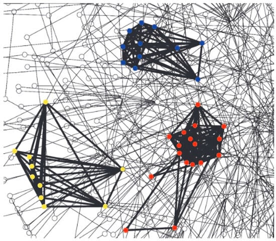
Figure 1.
Fragment of the protein network, nodes, and interactions in discovered clusters are shown in bold. Nodes are colored by functional categories in MIPS ; red, transcription regulation; blue, cell cycle/cell fate control; green, RNA processing; and yellow, protein transport [13]. Reprinted with permission from Ref. [13], Copyright 2003 Victor Spirin and Leonid A. Mirny.
Cliques inside an image are used in [15] to compute clique potentials with the objective of segmenting the entire image. A brain tumor picture receives treatment as a graph segment in [16], which uses a clique-based strategy to perform multi-modal segmentation of brain tumors. Additionally, Ref. [17] analyzes the brain’s synaptic networks and finds a large number of neuron cliques within gaps that facilitate correlated activity (see Figure 2).
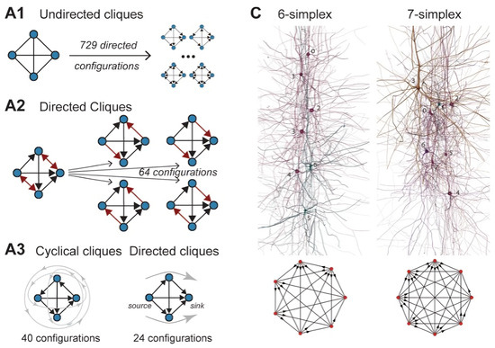
Figure 2.
Examples of neurons forming high-dimensional simplices in the reconstruction and their representation as directed graphs [17].
Cliques are another way that social networks identify groups of people who are acquainted with each other. Group members (or cliques) may have asymmetric relationships with anyone outside the group, while symmetric ties with one another belong to all by members. This is due to the fact that some individuals outside the clique are not connected at all, while others may be connected by an edge, implying exclusive relationships. The maximum clique constrained to visibility graphs of a simple polygon, computed using dynamic programming, is described in [18] (see Figure 3).
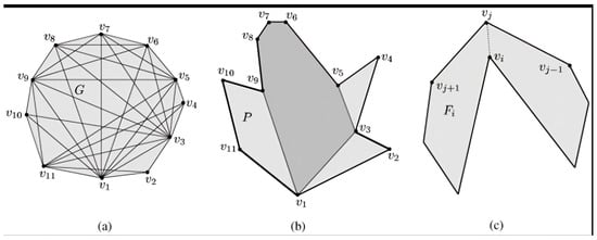
Figure 3.
The maximum clique in G and vertices of the largest convex polygon in P consist of vertices , which are shown in (a) and (b), respectively. (c) No vertex of can see any vertex of in the fan .
In [19], it is restricted to one-planar graphs, in [20] to dense graphs, and in [21] to graphs without long cycles. To generate different partitions on graphs, Tomescu et al. [22] employed counting, sequence, and layer matrices, along with proposed modifications and extensions. These partitions were then used to produce visual representations of the graphs.
A numerical semigroup is a cofinite subset of non-negative integers having additive binary operation and identity element. If , we can view the submonoid of , generated by X as
where . If is a numerical semigroup, then gcd. If no proper subset of X generates the numerical semigroup , then X is called the minimal set of generators and its cardinality is called embedding dimension e. The multiplicity m is the smallest non-zero element that belongs to the and the largest integer is called the Frobenius number . Rosales and Branco introduced that a numerical semigroup is irreducible if it is not expressible as the intersection of two numerical semigroups properly containing . Additionally, if a numerical semigroup has an odd Frobenius number and is irreducible, then it is symmetric. The main objective of this article is to propose a conjecture for the clique number of graphs associated with symmetric numerical semigroups of arbitrary multiplicity and embedding dimension and prove it for the case of
2. Clique Number of Graphs Associated with Symmetric Numerical Semigroups
In this section, we compute the clique number of , where is a symmetric numerical semigroup of arbitrary multiplicity and embedding dimension discussed in [23]. Let , then a graph associated with is said to be an induced subgraph of , represented by
Lemma 1
([24]). Let be a numerical semigroup with Then if and only if with and
Let , where and . We define the following sets as:
If is an odd integer, then we consider
or
and if or is an even integer, then
Proposition 1.
Let be a graph associated with numerical semigroup . Then , for every .
Proof.
Since , therefore . Furthermore, for , we have . Note that for every and ,
and for every
Above discussion implies for given conditions. Since is symmetric and is the Frobenius number of , therefore .
Now, we need to show that , are positive integers for given conditions. To show this, we consider the following cases:
- (1)
- For :
Since the maximum value of p is q, then
This implies , for .
- (2)
- For :
As the maximum value of t is , therefore
This gives , for .
- (3)
- For :
Note that for each a, the maximum of b is . Then,
since , therefore . This implies for and .
- (4)
- For :
If and , then
Now, if and , where , then
If q is odd, and , then
These imply that is a positive integer for all possibilities of a and b. Consequently, we obtain for every . □
Proposition 2.
Let be an induced subgraph of such that where . Then, .
Proof.
Since and , therefore This implies
We can write
This gives
Consider Since therefore . This implies Hence,
If m is even, then
Since and therefore and if m is odd, then
Since and therefore
To prove to be a complete graph, we have to show that
- Case 1:
- If and then
- Case 2:
- If and then
- Case 3:
- Let and Let where and Consider
- Case 4:
- Assume that , , then
- (1)
- and :
We can write
If q is even, then , and if q is odd, then and also, . This implies and and therefore
By Lemma 1, This gives
- (2)
- and :
It is easy to see that for every q and for each l, . This implies
If , then consider
where This implies
By Lemma 1,
Now, if , then consider
We can write
Note that
as By Lemma 1, . Furthermore, , from the above case. Consequently, we obtain .
- (3)
- q is odd, and :
Since and , therefore
If , then consider
This implies
By using Lemma 1, we obtain
Now, if , then consider
We can write
Note that
By using Lemma 1, . Furthermore, , from the above case. Consequently, we obtain . □
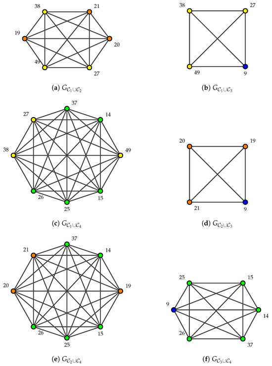
Example 1.
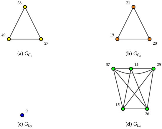
Let be a graph associated with then By Proposition 2, , , and The corresponding graphs are shown in Figure 4.
Figure 4.
The graphs associated with vertex partitions of numerical semigroup .
Proposition 3.
Let be an induced subgraph of such that , where . Then
Proof.
If , then consider
This implies
Now, if , then consider
We can write
Note that
By Lemma 1, . Furthermore, . Consequently, we obtain .
Since where then If then consider
This implies
So, we obtain
If then consider
This implies
So, we obtain
If , then consider
This implies
Now, if , then consider
We can write
Note that
By Lemma 1, . Furthermore, . Consequently, we obtain .
If then consider
This implies
So, we obtain
To prove is a complete graph where , we have to show that for and
- Case 1:
- If and , where and , where then
- Case 2:
- If and , where and then
Now, if , then consider
We can write
Note that
because This implies . Furthermore, . Consequently, we obtain .
- Case 3:
- If and , where and then
- (1)
- and :We can see that therefore Hence
- (2)
- , and or :
If then If then consider We can write
Note that
By Lemma 1, . Furthermore, . Consequently, we obtain .
- Case 4:
- If and , where and , then
Now, if , then consider
We can write
Note that
as This implies . Furthermore, . Consequently, we obtain .
- Case 5:
- If and , where and then
- Case 6:
- If and , where and then
Now, if , then consider
We can write
Note that
This implies . Furthermore, . Consequently, we obtain .
□
Example 2.
Let be a graph associated with , then
By Proposition 3, , , and The corresponding graphs are shown in Figure 5, respectively.
Figure 5.
The complete graphs associated with for .
Theorem 1.
Let be an induced subgraph of such that . Then, Moreover,
- 1.
- , if is odd.
- 2.
- if or is even.
Proof.
This follows from Proposition 3 that so we need to show for . For this, we have to discuss the following cases:
- Case 1:
- If , then t is not a minimal generator, which is a contradiction. Therefore and must be disjoint sets. Similar reasons imply and
- Case 2:
- If , then . Since therefore . As we know that and , therefore and are disjoint.
- Case 3:
- If , then and therefore . If then this gives and , which is a contradiction. If then , and gcd, therefore This gives , which is a contradiction as . This implies and are disjoint.
- Case 4:
- If , then . If , then , which is a contradiction, as j is a generator. If then . Since therefore and we also know that . Therefore,
This implies , and therefore
It is easy to see that if is odd then
if or is even then
□
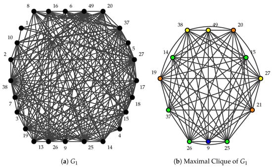
Conjucture: Let be a graph associated with numerical semigroup . If is odd then
and if or is even then
We prove this conjucture for the case, when . For this, we only need to show that is a maximal clique of .
Theorem 2.
Let , then is a maximal clique of .
Proof.
Since (by Lemma 1), therefore
Since therefore
Since (by Lemma 1), therefore
Since , therefore
Since (by Lemma 1), therefore
Since (by Lemma 1), therefore □
Let , where
- Case-1:
- If then for
- Case-2:
- If then
- Case-3:
- If then for
- Case-4:
- If and , then
- Case-5:
- If , , and , then
- Case-6:
- If , and , then
3. Discussion
In this work, we proposed a conjecture for the clique number of graphs associated with symmetric numerical semigroups of arbitrary multiplicity and embedding dimension. We elaborate this conjecture to relate back to the existing results characterizing the structural and algebraic properties of numerical semigroups dictated by their ass-commutation, which would further clarify some of these deeply involved connections with graph theory. We give evidence of this claim by studying a large number of examples of symmetric numerical semigroups with arbitrary multiplicities and embedding dimensions. The conjecture is supported extremely well by empirical data, and the proposed function turns out to be a very good predictor of the clique number in these cases. We have also verified the conjecture with computational techniques for a wider range of numerical semigroups giving our points another layer of evidence in favor of this hypothesis. The main focus for future research is to mathematically prove our conjecture. This will involve thoroughly studying the structure of symmetric numerical semigroups and their graphs, as well as developing new theoretical approaches and methods, and while our conjecture mainly applies to symmetric numerical semigroups, it would also be valuable to explore if similar outcomes can be obtained for non-symmetric numerical semigroups. Examining this wider category might uncover more connections and characteristics, thus enhancing the theory as a whole.
4. Conclusions
In this article, we compute the maximal clique of graphs associated with symmetric numerical semigroup of arbitrary multiplicity and embedding dimension 7. Moreover, we give a conjecture on the clique number of where is a symmetric numerical semigroup of arbitrary multiplicity and embedding dimension. In the future, we will compute the clique number of other classes of numerical semigroups and on this basis we will discuss the several invariants of .
Author Contributions
Conceptualization, M.A.B. and M.M.; methodology, M.M.; software, M.A.B.; validation, M.A.B., M.M. and A.S.A.; formal analysis, M.M.; investigation, M.A.B.; resources, A.S.A.; data curation, M.A.B.; writing—original draft preparation, M.M. and A.S.A.; writing—review and editing, M.A.B.; visualization, M.M.; supervision, M.A.B.; project administration, A.S.A.; funding acquisition, A.S.A. All authors have read and agreed to the published version of the manuscript.
Funding
This research was funded by Princess Nourah bint Abdulrahman University under Researchers Supporting Project Number (PNURSP2024R231).
Data Availability Statement
Data is contained within the article.
Acknowledgments
The authors extend their appreciations to Princess Nourah bint Abdulrahman University for funding this research under Researchers Supporting Project Number (PNURSP2024R231), Princess Nourah bint Abdulrahman University, Riyadh, Saudi Arabia.
Conflicts of Interest
The authors declare no conflicts of interest.
References
- Hashemi, E.; Alhevaz, A.; Yoonesian, E. On zero divisor graph of unique product monoid rings over Noetherian reversible ring. Categ. Gen. Algebr. Struct. Appl. 2016, 4, 95–114. [Google Scholar]
- Shen, R. Intersection graphs of subgroups of finite groups. Czechoslov. Math. J. 2010, 60, 945–950. [Google Scholar] [CrossRef][Green Version]
- Yaraneri, E. Intersection graph of a module. J. Algebra Appl. 2013, 12, 1250218. [Google Scholar] [CrossRef]
- Anderson, D.F.; Livingston, P.S. The Zero-Divisor Graph of a Commutative Ring. J. Algebra 1999, 217, 434–447. [Google Scholar] [CrossRef]
- Kumar, B.D.; Ajay, S.; Rahul, D. Nilpotent Graph. Theory Appl. Graphs 2021, 8, 2. [Google Scholar]
- Meier, J. Groups Graphs and Trees: An Introduction to the Geometry of Infinite Groups; Cambridge University Press: Cambridge, UK, 2008. [Google Scholar]
- Binyamin, M.A.; Siddiqui, H.M.A.; Khan, N.M.; Aslam, A.; Rao, Y. Characterization of graphs associated with numerical semigroups. Mathematics 2019, 7, 557. [Google Scholar] [CrossRef]
- Rao, Y.; Binyamin, M.A.; Aslam, A.; Mehtab, M.; Fazal, S. On the planarity of graphs associated with symmetric and pseudo symmetric numerical semigroups. Mathematics 2023, 11, 1681. [Google Scholar] [CrossRef]
- Cong, J.; Smith, M.L. A parallel bottom-up clustering algorithm with applications to circuit partitioning in VLSI design. In Proceedings of the 30th International Design Automation Conference, Dallas, TX, USA, 14–18 June 1993; pp. 755–760. [Google Scholar]
- Szabó, S.; Zaválnij, B. Graph Coloring via Clique Search with Symmetry Breaking. Symmetry 2022, 14, 1574. [Google Scholar] [CrossRef]
- Seda, M. The Maximum Clique Problem and Integer Programming Models, Their Modifications, Complexity and Implementation. Symmetry 2023, 15, 1979. [Google Scholar] [CrossRef]
- Vorobev, S.; Kolosnitsyn, A.; Minarchenko, I. Determination of the Most Interconnected Sections of Main Gas Pipelines Using the Maximum Clique Method. Energies 2022, 15, 15020501. [Google Scholar] [CrossRef]
- Spirin, V.; Mirny, L.A. Protein complexes and functional modules in molecular networks. Proc. Natl. Acad. Sci. USA 2003, 100, 12123–12128. [Google Scholar] [CrossRef]
- Samudrala, R.; Moult, J. A graph-theoretic algorithm for comparative modeling of protein structure. J. Mol. Biol. 1998, 279, 287–302. [Google Scholar] [CrossRef]
- Kato, Z.; Zerubia, J. Markov random fields in image segmentation. Found. Trends® Signal Process. 2012, 5, 1–155. [Google Scholar] [CrossRef]
- Liu, S.; Song, Y.; Zhang, F.; Feng, D.; Fulham, M.; Cai, W. Clique identification and propagation for multimodal brain Tumor image segmentation. In Proceedings of the Brain Informatics and Health: International Conference, Omaha, NE, USA, 13–16 October 2016; pp. 285–294. [Google Scholar]
- Reimann, M.W.; Nolte, M.; Scolamiero, M.; Turner, K.; Perin, R.; Chindemi, G.; Markram, H. Cliques of neurons bound into cavities provide a missing link between structure and function. Front. Comput. Neurosci. 2017, 11, 48. [Google Scholar] [CrossRef]
- Ghosh, S.K.; Shermer, T.C.; Bhattacharya, B.K.; Goswami, P.P. Computing the maximum clique in the visibility graph of a simple polygon. J. Discret. Algorithms 2007, 5, 524–532. [Google Scholar] [CrossRef]
- Gollin, J.P.; Hendrey, K.; Methuku, A.; Tompkins, C.; Zhang, X. Counting cliques in 1-planar graphs. Eur. J. Comb. 2023, 109, 103654. [Google Scholar] [CrossRef]
- Hedman, B. The maximum number of cliques in dense graphs. Discret. Math. 1985, 54, 161–166. [Google Scholar] [CrossRef][Green Version]
- Luo, R. The maximum number of cliques in graphs without long cycles. J. Comb. Theory Ser. B 2018, 128, 219–226. [Google Scholar] [CrossRef]
- Tomescu, M.A.; Jäntschi, L.; Rotaru, D.I. Figures of graph partitioning by counting, sequence and layer matrices. Mathematics 2021, 9, 1419. [Google Scholar] [CrossRef]
- Rosales, J. Symmetric numerical semigroups with arbitrary multiplicity and embedding dimension. Proc. Am. Math. Soc. 2002, 129, 2197–2203. [Google Scholar] [CrossRef]
- García-Sánchez, P.A.; Rosales, J.C. Numerical semigroups generated by intervals. Pasific J. Math. 1999, 191, 75–83. [Google Scholar] [CrossRef]


Disclaimer/Publisher’s Note: The statements, opinions and data contained in all publications are solely those of the individual author(s) and contributor(s) and not of MDPI and/or the editor(s). MDPI and/or the editor(s) disclaim responsibility for any injury to people or property resulting from any ideas, methods, instructions or products referred to in the content. |
© 2024 by the authors. Licensee MDPI, Basel, Switzerland. This article is an open access article distributed under the terms and conditions of the Creative Commons Attribution (CC BY) license (https://creativecommons.org/licenses/by/4.0/).