Abstract
Solitary waves, inherent in nonlinear wave equations, manifest across various physical systems like water waves, optical fibers, and plasma waves. In this study, we present this type of wave solution within the integrable Mikhailov–Novikov–Wang (MNW) equation, an integrable system known for representing localized disturbances that persist without dispersing, retaining their form and coherence over extended distances, thereby playing a pivotal role in understanding nonlinear dynamics and wave phenomena. Beyond this innovative work, we examine the stability and modulation instability of its gained solutions. These new solitary wave solutions have potential applications in telecommunications, spectroscopy, imaging, signal processing, and pulse modeling, as well as in economic systems and markets. To derive these solitary wave solutions, we employ two effective methods: the improved Sardar subequation method and the (℧′/℧, 1/℧) method. Through these methods, we develop a diverse array of waveforms, including hyperbolic, trigonometric, and rational functions. We thoroughly validated our results using Mathematica software to ensure their accuracy. Vigorous graphical representations showcase a variety of soliton patterns, including dark, singular, kink, anti-kink, and hyperbolic-shaped patterns. These findings highlight the effectiveness of these methods in showing novel solutions. The utilization of these methods significantly contributes to the derivation of novel soliton solutions for the MNW equation, holding promise for diverse applications throughout different scientific domains.
1. Introduction
Nonlinear equations (NLEs) represent the intricate tapestry of natural phenomena, encapsulating the nuanced behaviors of heat, fluidity, and light propagation. Unlike their linear counterparts, which tread predictable paths, NLEs navigate the complex terrain of our world, revealing its richness and depth. In the realm of scientific inquiry, these equations become storytellers, weaving narratives of soliton’s lone waves that glide effortlessly through optical fibers and other communication networks. Their solutions unveil the enigmatic workings of diverse natural phenomena, inviting exploration and understanding. Whether it is the intense heat flow within a furnace or the mesmerizing patterns of light pulses, NLEs offer a potent narrative tool [1,2,3,4,5]. Among different NLEs, the MNW equation, a prominent integrable equation, arises within the domain of nonlinear waves and soliton theory, finding applications in a multitude of physical phenomena such as shallow water waves, plasma physics, and nonlinear optics [6,7]. Renowned for its integrability, the MNW equation facilitates exact soliton solutions and enables both analytical and numerical investigations. Selected for its relevance and importance, the MNW signifies the localized disturbances that endure without dispersing, preserving their shape and coherence over considerable distances, crucial for comprehending nonlinear dynamics and wave behaviors [8,9]. By comprehensively studying the soliton propagation of the MNW equation, we acquire significant insights into its activities and dynamics across various fields. This equation arises from the application of the perturbative symmetry method for the classification of integrable equations. It belongs to a hierarchical structure, with the Boussinesq equation being one of its members. The equation manifests in two main forms: dispersive and nondispersive. The dispersive form is significant in systems where wave dispersion profoundly influences wave dynamics, such as in fiber optics and water waves. On the other hand, the nondispersive form holds relevance in scenarios where nonlinearity predominantly governs wave behavior, and dispersion effects are negligible, such as in certain shock waves. This investigation will focus on unveiling the dispersive form, which is expressed as follows [10,11]:
where signifies the wave amplitude with denoting time and representing the spatial coordinate; the terms , and represent the nonlinear interactions among the wave components. The incorporation of these nonlinear terms alongside high-order derivatives serves to reinforce the dispersive characteristics of the equation; the term indicates that the equation captures alterations in the curvature of the wave profile as time progresses, which is a characteristic feature of dispersive behavior; the term contributes to dispersion by introducing complexity into the evolution of the wave; and the terms , and indicate nonlinear interactions, which are typical in equations describing complex wave phenomena.
Because of the MNW equation’s unique properties and dynamics, this equation has captured the interest of researchers. Among various researchers, refs. [8,12] derived kink-type multi-soliton solutions of the equation employing the (G′/G)-expansion method and the simplified version of Hirota’s method, respectively. Using a unified approach, ref. [13] established some anti-bell and periodic solutions. Conversely, ref. [6] developed bright and periodic soliton solutions, along with numerical verification using three methods: the extended simple equation technique, He’s variational iteration technique, and the modified Riccati technique. Given the significant importance of this equation, various methodologies have been employed to derive exact solutions. However, this study aims to explore additional approaches to generate new types of solutions.
Due to the significant fascination and importance of finding exact solutions for NLEs, numerous scholars have employed several mathematical procedures to accomplish the goal. These techniques encompass the extension of the auxiliary equation mapping method [14], the technique [15], the modified exp-function approach [16], the Hirota bilinear method [17], the Riccati equation approach [18], the -expansion technique [19], the generalized exp-function approach [20], the functional variable technique [21], the fractional approach [22], the extension of the modified rational expansion approach [23,24], the first integral approach [25], the simple equation technique [26], the tanh–coth method [27], the generalized Kudryshov method [28], the unified method [29], the technique [30], and many others.
The improved Sardar subequation method’s advantage in discovering exact solutions lies in its capacity to simplify intricate nonlinear equations, making it easier to identify a wide array of soliton solutions efficiently. Specifically tailored for equations with one variable, it yields precise and diverse soliton patterns that might pose challenges for other methodologies. Widely utilized by researchers, it has proven effective in revealing analytical solutions for various NLEs [31,32,33,34,35,36]. On the other hand, the (, ) method operates with two variables. It provides a comprehensive framework for exploring various transformations and solution strategies, thereby offering insights into the behavior and properties of solutions. Notably, this method encompasses trigonometric, hyperbolic, and rational solutions, making it highly versatile [37,38,39,40,41].
Up to the present, there has not been any examination of the stated equation employing these two techniques. Additionally, exploring the aforementioned equation using both stability and modulation instability methods has been absent. Stability and modulation instability are pivotal phenomena observed in nonlinear systems. Stability refers to a substance’s ability to maintain its equilibrium despite disturbances, while modulation instability signifies the uncontrolled growth of oscillations or perturbations, leading to the formation of patterns or features within a system [42,43]. These analyses find wide-ranging applications across various fields such as nonlinear imaging, wavelength conversion, telecommunications, spectroscopy, optical coherence tomography, as well as economic systems and markets. Therefore, this study aims to employ these specified methodologies to derive exact solutions while examining the stability analysis and modulation instability of the given nonlinear equation. The manuscript is put in order as follows: (i) Section 2 supplies an overview of the methods. (ii) In Section 3, the methodological application of the MNW equation is provided. (iii) Several analyses of the main equation are presented in Section 4. (iv) Section 5 delves into visual representations with a discussion. (v) A comparison is presented in Section 6. (vi) The conclusion is shown in Section 7 and at the end of this manuscript, a bibliography comprising references is appended.
2. Mathematical Approach
2.1. Improved Sardar Subequation Approach
In this section, we delve into the improved Sardar subequation method, renowned for its efficacy in deriving precise solutions to a range of NLEs [32,44,45]. As we embark on this analytical exploration, let us consider the broad framework of NLEs, typically characterized by two distinct independent variables, and , as follows:
where is a polynomial and , , , , , ….
Now, assume a new variable, , governed by the following succeeding relationship:
where represents the speed of the soliton.
Thus, by employing Equation (3) to Equation (2), we can convert it into an ordinary differential equation (ODE), structured as follows:
Top of Form
In this context, the symbol represents a novel polynomial incorporating alongside its ordinary derivatives ().
The equation describing the subsequent general solution is as follows:
Top of Form
succeeding in the following:
In Equation (6), the symbol ‘’ denotes differentiation with respect to , while (i = 1, 2, 3, ..., n), , and are arbitrary constants. Here, the parameter n is the balancing constant to be determined and represents a positive integer.
The solutions derived from Equation (6) are contingent upon the properties of the parameters ( and ) and are manifested as follows:
Scenario I. When but , then
where and .
Scenario II. When but , then
where and .
Scenario III. When but , then
where and .
Scenario IV. When but , then
where and .
In Equations (7)–(20), the parameters and are nonzero-free arbitrary real values. When or , the given equations transform into known trigonometric and hyperbolic forms and the solution offered by Equation (15) corresponds to the solution provided by Equation (12), and the solutions given by Equations (19) and (20) correspond to the solution offered by Equation (17), i.e., and
Next, we proceed to the subsequent steps aimed at deriving exact solutions for the NLEs:
Method’s Workflow
To determine the balance number , we employ the homogeneous balance method. By switching the value of into Equation (5) and subsequently merging this into Equation (4), utilizing Equation (6), the left-hand side of Equation (4) is converted into a polynomial containing terms with . Setting the coefficients of each term with matching powers in the polynomial to zero establishes a system containing , and . By solving these systems, the unknown coefficients, denoted as , are determined. Substituting these coefficients into Equation (5) yields exact solutions for Equation (1) in 14 different forms.
2.2. The (, ) Approach
Here, we offer an extensive guide to the fundamental steps involved in employing the method, originally introduced by [46]. To analyze the NLEs described in Equation (2), we utilize the transformation variable outlined in Equation (3). This transformation enables us to convert the NLEs into ODEs, facilitating a more straightforward analytical treatment [47,48]. The ODE associated with this method can be expressed as follows:
where ‘’ is the derivative concerning .
The two new variables within this method can be defined as follows:
subsequent correspondences are as follows:
The result of Equation (21) differs depending on λ, which falls into three separate scenarios:
Scenario I. If :
The general solution of this case is as follows:
which generates the following:
where .
Scenario II. If :
Similarly, like the previous case, the general solution is written as follows:
subsequent in the following:
where .
Scenario III. If :
Similarly:
Which gives the following:
Therefore, Equation (4) yields the following general solution:
where, , , and (i = 1, 2, 3,…, p) denote unknown coefficients, ensuring that . The parameter signifies that the balance number needs to be figured out.
Method’s Workflow for Computing Exact Solutions:
- Substitute the determined value of into Equation (30) and then substitute in Equation (4), along with Equations (22), (23) and (25). This transformation yields a polynomial in the left-hand side of Equation (30), incorporating terms and .
- Formulate a system of algebraic equations by equating the coefficients of terms with corresponding powers within the polynomial to 0. These equations include parameters such as , , , , , and others.
- Any symbolic calculation tools can solve these algebraic equations, thereby determining the values of the involved parameters.
- Substitute the obtained parameter values into Equation (30), expressed in trigonometric, hyperbolic, and rational functions that are the exact solution of Equation (1).
3. Method’s Application
Upon applying the transformation outlined in Equation (3) to Equation (1), the equation undergoes the following transformation:
After integrating the ODE as mentioned above and setting the constant of integration to zero, the resulting equation is given by the following:
Suppose
Alternatively, Equation (33) is represented by the following:
Equation (34) has been solved in the following subsections to extract soliton solutions using the previously outlined schemes.
3.1. The Improved Sardar Subequation Method
Employing the balancing principle in Equation (34), we get the balance number ; the solution takes on the following structure:
Within this equation, the constants , , and represent coefficients that need to be determined. By following the outlined methodology, we derive a set of algebraic equations (see Appendix A), which we subsequently solve to determine the unknown coefficients as follows:
and
Utilizing Equations (5), (6) and (35)–(37), the solutions for Equation (1) are derived as follows:
Scenario I. When but , then
Scenario II. When but , then
Top of Form
Scenario III. When but , then
or
Scenario IV. When but , then
or
3.2. The (, ) Approach
Again, applying the balance principle in Equation (34) that provides , the solution takes on the following structure in this approach:
The equation needs the determination of the coefficients , , and , as well as and
Scenario I. For trigonometric solutions ().
Following the methodology outlined in the methodology section, we have derived a set of algebraic equations (see Appendix B). Solving this system yields the values of the coefficients as follows:
Now, collectively, Equations (34), (56) and (57) yield:
Setting both and to zero, however, confirming is non-zero, Equation (58) converts into the following format:
Scenario II. For hyperbolic solutions ().
Similarly, for this scenario, we have derived a set of algebraic equations (see Appendix C). Solving this system provides the values of the coefficients as follows:
Top of Form
Similarly, as in the earlier case:
Top of Form
Scenario III. If (rational solutions).
Using the outlined methodology, we formulate a set of algebraic equations (see Appendix D). Solving these equations provides us with the velocity, is zero, which is not physically feasible. This indicates that there is no valid solution for this particular case.
4. Analyses
In this section, we aim to examine both the stability analysis and modulation instability analysis of the derived solution.
4.1. Stability Analysis
The stability analysis is of fundamental importance across various disciplines such as system control and signal processing. It typically pertains to understanding the behavior of dynamic systems, which can span mechanical, electrical, or chemical domains in the natural world. In the case of Equation (1), the Hamiltonian and momentum associated with this approach are described as follows [49,50]:
wherein denotes the momentum and means the electrical potential. To check stability, the following inequalities must be satisfied:
where represents the frequency.
Now, this phenomenon is applied to one of the solutions, such as Equation (39), for the fixed value of (we can choose any real value of ), which yields the following:
Oversimplification yields the following:
Exploiting the stabilization in Equation (63) yields the following:
Given the conditions outlined in Equation (63), the stability of the solution obtained in Equation (39) is clearly demonstrated by Equation (66), indicating that Equation (1) exhibits nonlinear stability for any real value of . Through a similar process, we can conduct a stability analysis of other solutions.
4.2. Modulation Instability
Modulation instability exemplifies the unconfined progress of perturbations or fluctuations in a system. In this subsection, modulation instability is thoroughly checked for the MNW equation. At this point, we assume the perturbed solution as follows [49,50]:
where stands for a steady flow attitude for Equation (1). By relating Equation (67) to Equation (1), while linearizing in , this yields the following:
We can assume that the solution of Equation (68) is of the following form:
where and represent the waveform quantity and the frequency, respectively.
Equations (68) and (69) jointly provide the following:
From the above equation, we can write the following:
Equation (71) always supplies the negative value. From this consequence, we confirmed that any arrangement of the soliton solutions showed a decaying configuration. So, a stable dispersion is discovered in the suggested model.
5. Visual Representation of the Exact Solutions
Using Mathematica, we explored the intricate graphical shapes displayed by the MNW equation employing both methods. Our exposition contained a diverse range of visualizations, including 3D, 2D, and contour depictions. These visual representations spanned various parameter values, providing a comprehensive insight into the graphical behavior of the MNW equation.
To ensure clarity and conciseness, we have selected four representative solutions for the improved Sardar subequation method and three sets for the (, ) method from our extensive results for visualization. These graphs are depicted over fitting intervals, specifically for each case, with the corresponding constants provided in the figure descriptions. In the 2D plots, various depictions were amalgamated into a unified figure by altering the parameter t.
5.1. Visualization via Improved Sardar Subeqaution Method
Figure 1, Figure 2, Figure 3 and Figure 4 are from Improve Sardar Subequation Method. Please check the following figures.
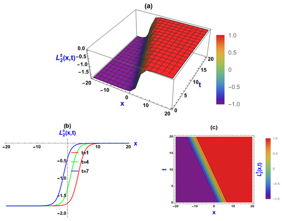
Figure 1.
Depiction of for , and : (a) 3D view of an anti-kink soliton, (b) 2D view of an anti-kink soliton, and (c) contour view of an anti-kink soliton.

Figure 2.
Depiction of for , and : (a) 3D view of the singular solitons, (b) 2D view of the singular solitons, and (c) contour view of the singular solitons.
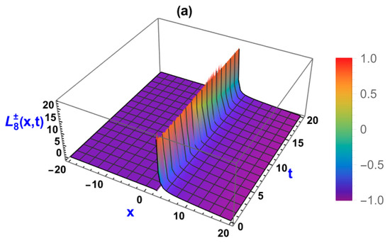
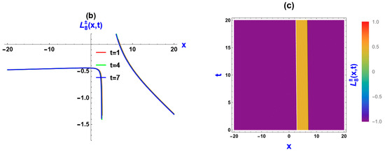
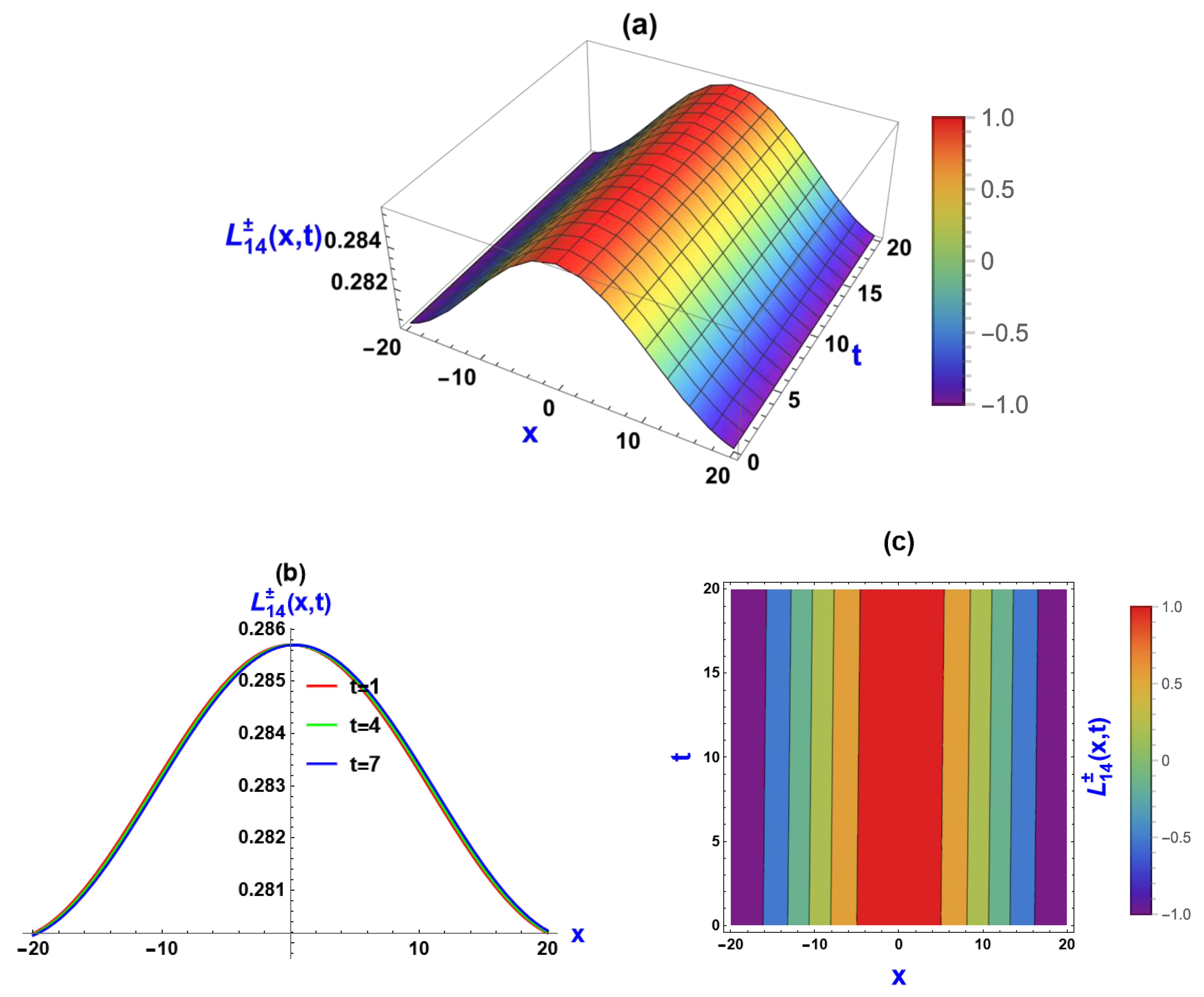
Figure 3.
Depiction of for , and : (a) 3D depiction of the breather soliton, (b) 2D depiction of the breather soliton, and (c) contour depiction of the breather soliton.

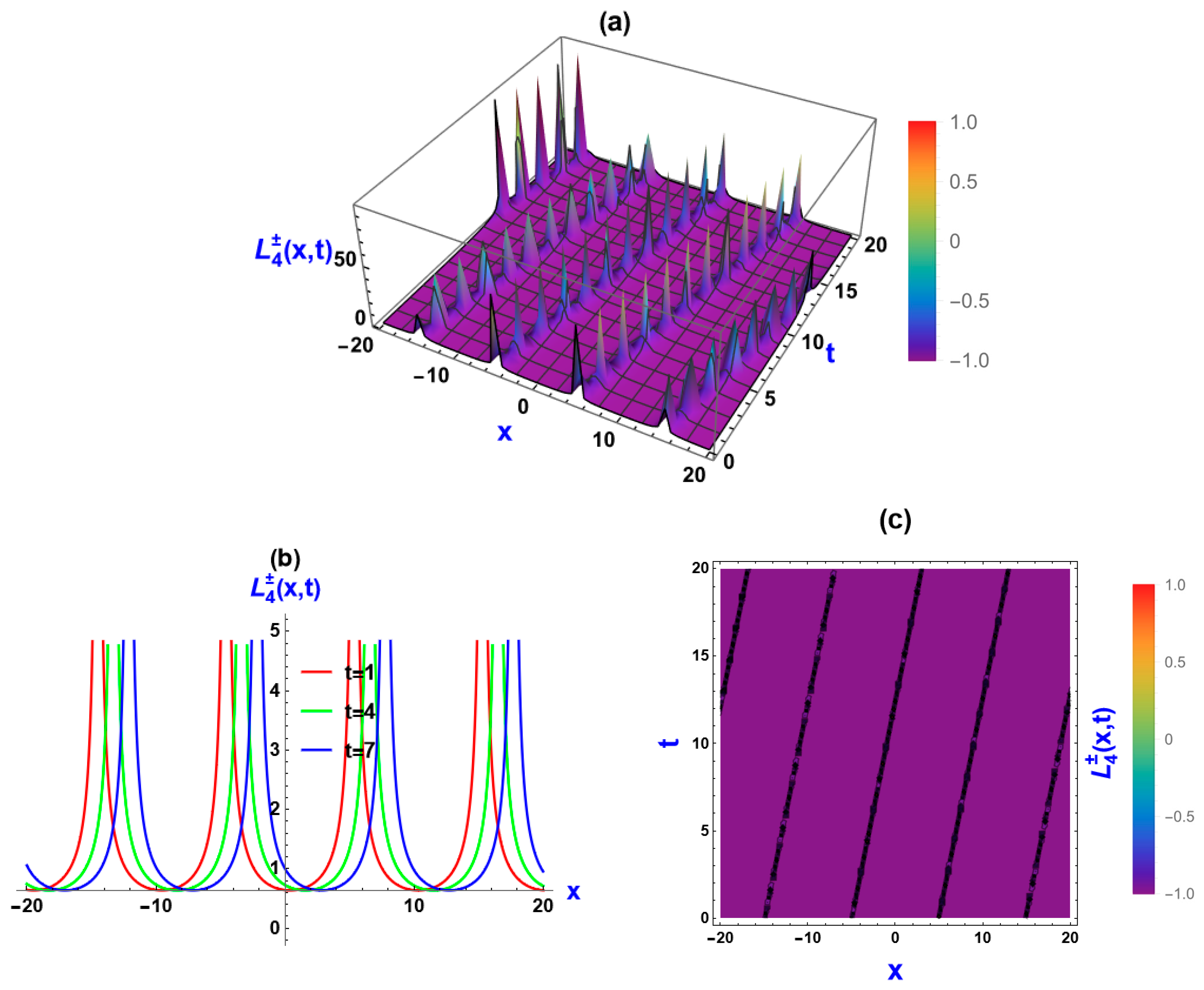
Figure 4.
Depiction of for , and : (a) 3D view of the bell-shaped solitons, (b) 2D view of the bell-shaped solitons, and (c) contour view of the bell-shaped solitons.
5.2. Visualization via (, ) Approach
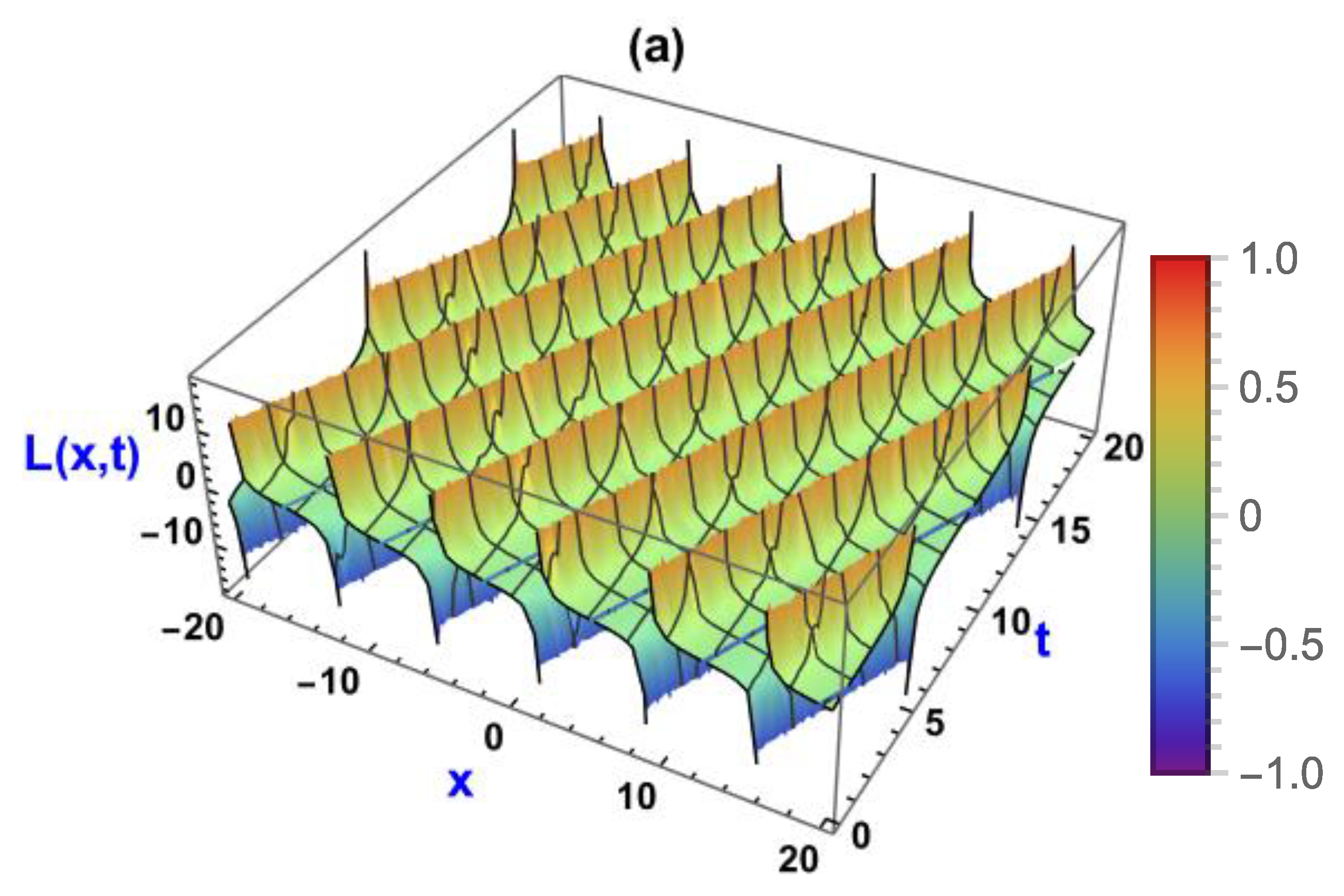
Figure 5.
Depiction of Equation (68) for , and : (a) 3D view of the multi-singular solitons, (b) 2D view of the multi-singular solitons, and (c) contour view of the multi-singular solitons.
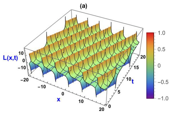
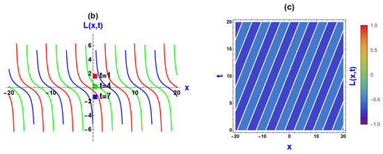
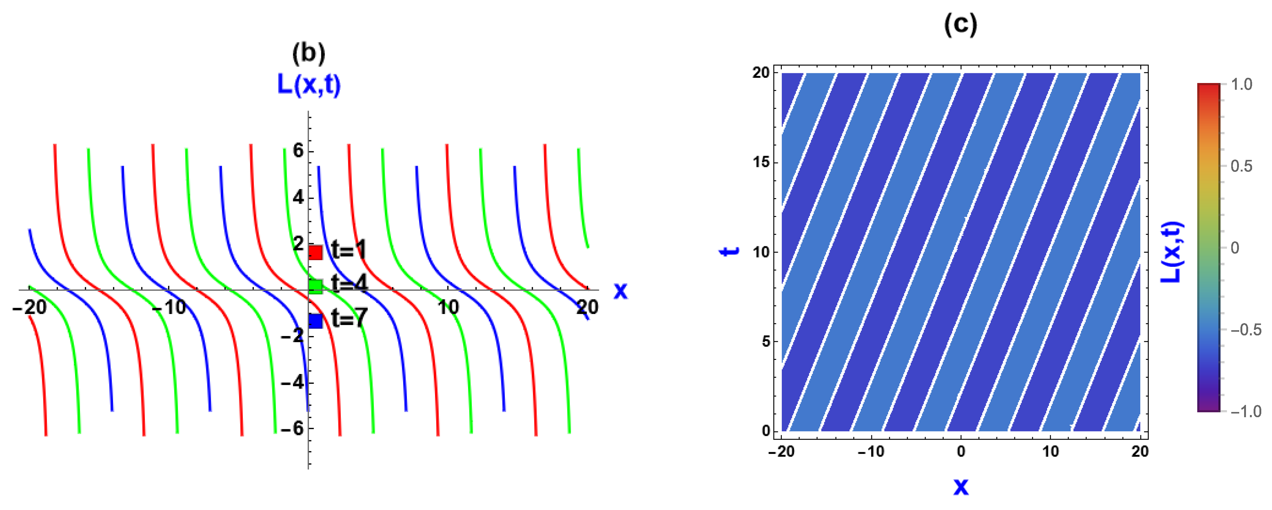
Figure 6.
Depiction of Equation (69) for : (a) 3D view of the kink solitons, (b) 2D view of the kink solitons, and (c) contour view of the kink solitons.

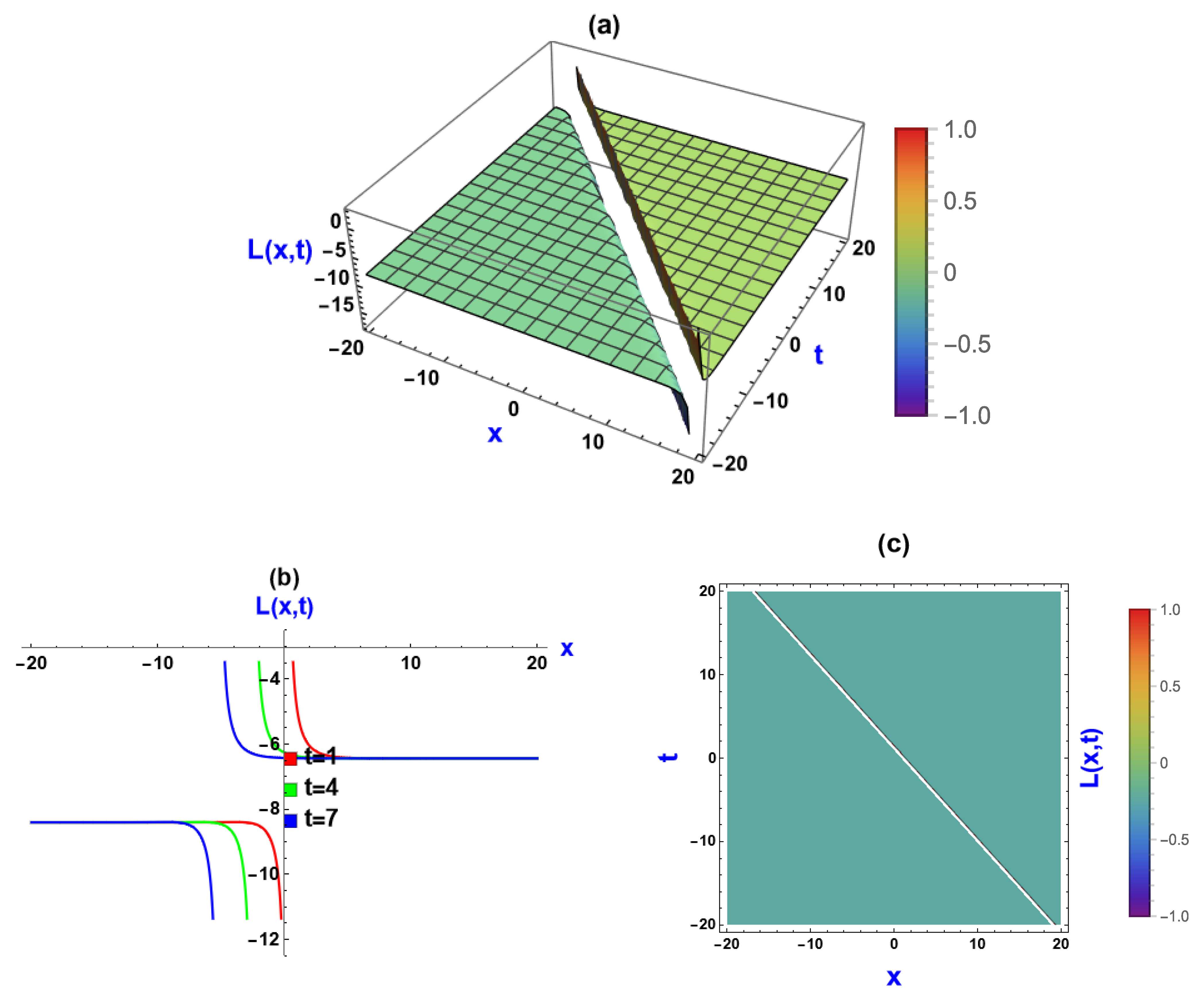
Figure 7.
Depiction of Equation (73) for and : (a) 3D view of the hyperbolic soliton, (b) 2D view of the hyperbolic soliton, and (c) contour 3D view of the hyperbolic soliton.
5.3. Discussions of the Graphs
The figures presented in this study depict various soliton structures obtained through two distinct methodologies: the improved Sardar subequation technique and the (, ) method. Focusing first on Figure 1, Figure 2, Figure 3 and Figure 4, which utilize the improved Sardar subequation technique, we observe a range of soliton behaviors. Figure 1 effectively illustrates the anti-kink soliton solution, while Figure 2 showcases the singular soliton. In Figure 3, we prominently observe characteristics of the breather solitons. Conversely, Figure 4 illustrates an anti-kink soliton structure. These visualizations are primarily influenced by the parameter , where positive values yield kink solitons, while negative values lead to the breather and singular solitons.
Turning attention to Figure 5, Figure 6 and Figure 7, derived using the (, ) method, we meet a different set of soliton structures, where Figure 5 illustrates the singular soliton solution, Figure 6 shows multi-singular soliton characteristics, and Figure 7 showcases the hyperbolic soliton structure. In this methodology, the dominant parameter influencing soliton behavior is , which acts as a wave speed in the model solution and is also responsible for the soliton behavior of the model.
Our exploration of soliton solutions from Equation (1) yields various types, including kink, ant-kink, bell, breather, multi-singular, hyperbolic, periodic, and singular solitons. These solutions play vital roles across diverse fields, providing deep insights into system dynamics and physics principles. Applications range from condensed matter physics, where kink and anti-kink solitons impact magnetic domain dynamics, to nonlinear optics; the breather soliton enables the generation of stable, localized light pulses that propagate over long distances in optical fibers with minimal distortion. Additionally, multiple singular and hyperbolic solitons find utility in fluid dynamics and plasma physics, while kink solitons with regular singularities aid in predicting extreme wave events. Furthermore, the bell soliton is applied to model stable, compact solitary waves in nonlinear wave equations, which is essential for describing localized structures across diverse physical systems. Overall, these soliton solutions advance science, technology, and engineering, enhancing our understanding of natural phenomena and driving technological innovation.
6. Comparison
This section delves into the originality and scientific significance of our discoveries by conducting a comparative analysis of the findings presented in the studies by [8,11,12]. This contrast is designed into two separate sections, carefully exploring the similarities and differences between our respective research endeavors. By highlighting both the shared aspects and discrepancies, our goal is to offer a thorough insight into the distinct contributions of our research concerning the existing works.
6.1. Unities
- (a)
- Both this study and previous studies focus on the MNW equation, a pivotal nonlinear model utilized for analyzing solitary wave dynamics.
- (b)
- The primary objective of both studies is to attain precise exact solutions through the utilization of analytical techniques.
- (c)
- Both studies have discovered a shared soliton type, specifically the kink soliton.
6.2. Variation and Uniqueness
- (a)
- In this study, two versatile methods were employed: the improved Sardar subequation method (involving one variable) and the (, ) method (utilizing two variables). Conversely, other studies utilized diverse methodologies, such as the (G′/G)-expansion method by [8], simplified Hirota’s method by [12], singular manifold method, exp(−(ξ))-expansion method, and generalized projective Riccati equations method by [11].
- (b)
- While the previous studies primarily yielded kink, anti-kink, bright, and periodic solitons, our investigation encompasses a broader range of soliton patterns. We have identified breather, singular, kink, anti-kink, bell, and hyperbolic-shaped solitons, among which singular, breather, bell, and hyperbolic-shaped solitons are entirely novel.
- (c)
- This study addresses both stability and modulation stability, whereas these critical aspects were overlooked in other studies.
7. Conclusions
In this study, a series of novel exact solitary wave solutions to the MNW equation were uncovered using two versatile methods: the improved Sardar subequation method (one variable) and the (, ) method (two variables). Through these methods, a diverse range of solutions were constructed, spanning rational, trigonometric, and hyperbolic functions. Additionally, both stability analysis and modulation instability analysis have been effectively conducted, confirming the stability (nonlinearly stable and following a stable dispersion pattern) of the derived solution within this model. The solution achieved in this investigation comprises a spectrum of soliton patterns, encompassing dark, singular, kink, anti-kink, and hyperbolic-shaped solitons, which deviate from conventional methodologies, offering a more precise portrayal of the dynamic behavior governed by the MNW equation. The utilization of computational techniques notably led to the revelation of a novel type of soliton solution for the MNW equation. Within this study, the identification of bell, breather, hyperbolic, and singular soliton types represents a significant advancement with broad applications in fluid dynamics and optical and plasma physics. Various manifestations of these solutions, depicted through contour, 2D, and 3D plots, accentuate their diversity. These soliton solutions present promising prospects for advancing technology and engineering, fostering a deeper comprehension of natural phenomena, and nurturing innovation within the realm of the MNW equation. These discoveries not only promise to augment technological capabilities but also contribute to a profound understanding of intricate nonlinear dynamics.
Author Contributions
Conceptualization, M.N.H., M.S.A., K.E.-R. and J.R.M.B.; methodology, M.N.H., M.S.A., K.E.-R., M.M.M. and M.K.; software, M.M.M. and J.R.M.B.; validation, M.N.H., M.M.M. and M.K.; investigation, M.N.H., M.S.A., K.E.-R., J.R.M.B. and M.K.; writing—original draft, M.N.H., M.S.A., K.E.-R., J.R.M.B. and M.M.M.; writing—review and editing, M.N.H., M.M.M. and M.K.; supervision, M.M.M. and M.K. All authors have read and agreed to the published version of the manuscript.
Funding
This research was funded by the Deanship of Graduate Studies and Scientific Research, Taif University.
Institutional Review Board Statement
I hereby declare that this manuscript is the result of my independent creation under the reviewers’ comments. Except for the quoted contents, this manuscript does not contain any research achievements that have been published or written by other individuals or groups.
Data Availability Statement
All data generated or analyzed during this study are included in this article.
Acknowledgments
The authors would like to acknowledge the Deanship of Graduate Studies and Scientific Research, Taif University for funding this work.
Conflicts of Interest
The authors declare no conflicts of interest.
Appendix A
Substituting Equation (35) into Equation (34), taking into account the derivative relationship given by Equation (6), provides a polynomial form according to , . Taking into account the identity of the polynomial to zero, the following system of algebraic equations is obtained:
For improved Sardar subequation method:
Appendix B
Similarly, we derived the following system of equations for the (, ) method:
For
Appendix C
For
Appendix D
For
References
- Zafar, A.; Raheel, M.; Ali, K.K.; Razzaq, W. On Optical Soliton Solutions of New Hamiltonian Amplitude Equation via Jacobi Elliptic Functions. Eur. Phys. J. Plus 2020, 135, 674. [Google Scholar] [CrossRef]
- Hossain, M.N.; Miah, M.M.; Hamid, A.; Osman, G.M.S. Discovering New Abundant Optical Solutions for the Resonant Nonlinear Schrödinger Equation Using an Analytical Technique. Opt. Quantum Electron. 2024, 56, 847. [Google Scholar] [CrossRef]
- Borhan, J.R.M.; Ganie, A.H.; Miah, M.M.; Iqbal, M.A.; Seadawy, A.R.; Mishra, N.K. A Highly Effective Analytical Approach to Innovate the Novel Closed Form Soliton Solutions of the Kadomtsev–Petviashivili Equations with Applications. Opt. Quantum Electron. 2024, 56, 938. [Google Scholar] [CrossRef]
- Seadawy, A.R.; Iqbal, M. Dispersive Propagation of Optical Solitions and Solitary Wave Solutions of Kundu-Eckhaus Dynamical Equation via Modified Mathematical Method. Appl. Math. 2023, 38, 16–26. [Google Scholar] [CrossRef]
- Seadawy, A.R.; Iqbal, M.; Althobaiti, S.; Sayed, S. Wave Propagation for the Nonlinear Modified Kortewege–de Vries Zakharov–Kuznetsov and Extended Zakharov–Kuznetsov Dynamical Equations Arising in Nonlinear Wave Media. Opt. Quantum Electron. 2021, 53, 85. [Google Scholar] [CrossRef]
- Khater, M.M.A. Soliton Propagation under Diffusive and Nonlinear Effects in Physical Systems; (1+1)–Dimensional MNW Integrable Equation. Phys. Lett. A 2023, 480, 128945. [Google Scholar] [CrossRef]
- Iqbal, M.; Lu, D.; Seadawy, A.R.; Ashraf, M.; Albaqawi, H.S.; Khan, K.A.; Chou, D. Investigation of Solitons Structures for Nonlinear Ionic Currents Microtubule and Mikhaillov-Novikov-Wang Dynamical Equations. Opt. Quantum Electron. 2024, 56, 361. [Google Scholar] [CrossRef]
- Bekir, A.; Shehata, M.S.M.; Zahran, E.H.M. Comparison between the New Exact and Numerical Solutions of the Mikhailov–Novikov–Wang Equation. Numer. Methods Partial Differ. Equ. 2024, 40, e22775. [Google Scholar] [CrossRef]
- Akbulut, A.; Kaplan, M.; Kaabar, M.K.A. New Exact Solutions of the Mikhailov-Novikov-Wang Equation via Three Novel Techniques. J. Ocean Eng. Sci. 2023, 8, 103–110. [Google Scholar] [CrossRef]
- Mikhailov, B.A.V.; Novikov, V.S.; Wang, J.P. On Classification of Integrable Davey-Stewartson Type Equations. Stud. Appl. Math. 2007, 118, 419–457. [Google Scholar] [CrossRef]
- Raza, N.; Seadawy, A.R.; Arshed, S.; Rafiq, M.H. A Variety of Soliton Solutions for the Mikhailov-Novikov-Wang Dynamical Equation via Three Analytical Methods. J. Geom. Phys. 2022, 176, 104515. [Google Scholar] [CrossRef]
- Ray, S.S.; Singh, S. New Various Multisoliton Kink-Type Solutions Ofthe (1 + 1)-Dimensional Mikhailov–Novikov–Wang Equation. Math. Methods Appl. Sci. 2021, 44, 14690–14702. [Google Scholar] [CrossRef]
- Kumar, A.; Kumar, S. Dynamic Nature of Analytical Soliton Solutions of the (1+1)-Dimensional Mikhailov-Novikov-Wang Equation Using the Unified Approach. Int. J. Math. Comput. Eng. 2023, 1, 217–228. [Google Scholar] [CrossRef]
- Seadawy, A.R.; Iqbal, M. Propagation Ofthe Nonlinear Damped Korteweg-de Vries Equation in an Unmagnetized Collisional Dusty Plasma via Analytical Mathematical Methods. Math Meth Appl Sci. 2021, 44, 737–748. [Google Scholar] [CrossRef]
- Mia, R.; Mamun Miah, M.; Osman, M.S. A New Implementation of a Novel Analytical Method for Finding the Analytical Solutions of the (2+1)-Dimensional KP-BBM Equation. Heliyon 2023, 9, e15690. [Google Scholar] [CrossRef] [PubMed]
- Shakeel, M.; Attaullah; Shah, N.A.; Chung, J.D. Modified Exp-Function Method to Find Exact Solutions of Microtubules Nonlinear Dynamics Models. Symmetry 2023, 15, 360. [Google Scholar] [CrossRef]
- Ma, W.X. N-Soliton Solutions and the Hirota Conditions in (1 + 1) -Dimensions. Int. J. Nonlinear Sci. Numer. Simul. 2022, 23, 123–133. [Google Scholar] [CrossRef]
- Elsayed, M.E.Z.; Khaled, A.E.A. The Generalized Projective Riccati Equations Method and Its Applications for Solving Two Nonlinear PDEs Describing Microtubules. Int. J. Phys. Sci. 2015, 10, 391–402. [Google Scholar] [CrossRef]
- Mohanty, S.K.; Kravchenko, O.V.; Deka, M.K.; Dev, A.N.; Churikov, D.V. The Exact Solutions of the 2+1–Dimensional Kadomtsev–Petviashvili Equation with Variable Coefficients by Extended Generalized [Formula Presented]-Expansion Method. J. King Saud Univ.-Sci. 2023, 35, 102358. [Google Scholar] [CrossRef]
- Shakeel, M.; Attaullah; Kbiri Alaoui, M.; Zidan, A.M.; Shah, N.A.; Weera, W. Closed-Form Solutions in a Magneto-Electro-Elastic Circular Rod via Generalized Exp-Function Method. Mathematics 2022, 10, 3400. [Google Scholar] [CrossRef]
- Babajanov, B.; Abdikarimov, F. The Application of the Functional Variable Method for Solving the Loaded Non-Linear Evaluation Equations. Front. Appl. Math. Stat. 2022, 8, 912674. [Google Scholar] [CrossRef]
- Tandel, P.; Patel, H.; Patel, T. Tsunami Wave Propagation Model: A Fractional Approach. J. Ocean Eng. Sci. 2022, 7, 509–520. [Google Scholar] [CrossRef]
- Iqbal, M.; Seadawy, A.R.; Lu, D.; Zhang, Z. Computational Approach and Dynamical Analysis of Multiple Solitary Wave Solutions for Nonlinear Coupled Drinfeld–Sokolov–Wilson Equation. Results Phys. 2023, 54, 107099. [Google Scholar] [CrossRef]
- Seadawy, A.R.; Zahed, H.; Iqbal, M. Solitary Wave Solutions for the Higher Dimensional Jimo-Miwa Dynamical Equation via New Mathematical Techniques. Mathematics 2022, 10, 1011. [Google Scholar] [CrossRef]
- Taghizadeh, N.; Mirzazadeh, M. The First Integral Method to Some Complex Nonlinear Partial Differential Equations. J. Comput. Appl. Math. 2011, 235, 4871–4877. [Google Scholar] [CrossRef]
- Islam, Z.; Sheikh, M.A.N.; Roshid, H.O.; Hossain, M.A.; Taher, M.A.; Abdeljabbar, A. Stability and Spin Solitonic Dynamics of the HFSC Model: Effects of Neighboring Interactions and Crystal Field Anisotropy Parameters. Opt. Quantum Electron. 2024, 56, 190. [Google Scholar] [CrossRef]
- Kumar, A.; Pankaj, R.D. Tanh–Coth Scheme for Traveling Wave Solutions for Nonlinear Wave Interaction Model. J. Egypt. Math. Soc. 2015, 23, 282–285. [Google Scholar] [CrossRef]
- Islam, S.; Khan, K.; Arnous, A.H. Generalized Kudryashov Method for Solving Some. New Trends Math. Sci. 2015, 57, 46–57. [Google Scholar]
- Abdel-Gawad, H.I.; Osman, M. On Shallow Water Waves in a Medium with Time-Dependent Dispersion and Nonlinearity Coefficients. J. Adv. Res. 2015, 6, 593–599. [Google Scholar] [CrossRef]
- Shakeel, M.; Manan, A.; Bin Turki, N.; Shah, N.A.; Tag, S.M. Novel Analytical Technique to Find Diversity of Solitary Wave Solutions for Wazwaz-Benjamin-Bona Mahony Equations of Fractional Order. Results Phys. 2023, 51, 106671. [Google Scholar] [CrossRef]
- Iqbal, I.; Rehman, H.U.; Mirzazadeh, M.; Hashemi, M.S. Retrieval of Optical Solitons for Nonlinear Models with Kudryashov’s Quintuple Power Law and Dual-Form Nonlocal Nonlinearity. Opt. Quantum Electron. 2023, 55, 588. [Google Scholar] [CrossRef]
- Rezazadeh, H.; Inc, M.; Baleanu, D. New Solitary Wave Solutions for Variants of (3+1)-Dimensional Wazwaz-Benjamin-Bona-Mahony Equations. Front. Phys. 2020, 8, 332. [Google Scholar] [CrossRef]
- Rehman, H.U.; Iqbal, I.; Subhi Aiadi, S.; Mlaiki, N.; Saleem, M.S. Soliton Solutions of Klein–Fock–Gordon Equation Using Sardar Subequation Method. Mathematics 2022, 10, 3377. [Google Scholar] [CrossRef]
- Ibrahim, S.; Ashir, A.M.; Sabawi, Y.A.; Baleanu, D. Realization of Optical Solitons from Nonlinear Schrödinger Equation Using Modified Sardar Sub-Equation Technique. Opt. Quantum Electron. 2023, 55, 617. [Google Scholar] [CrossRef]
- Cinar, M.; Secer, A.; Ozisik, M.; Bayram, M. Derivation of Optical Solitons of Dimensionless Fokas-Lenells Equation with Perturbation Term Using Sardar Sub-Equation Method. Opt. Quantum Electron. 2022, 54, 402. [Google Scholar] [CrossRef]
- Hossain, M.N.; Miah, M.M.; Alosaimi, M.; Alsharif, F.; Kanan, M. Exploring Novel Soliton Solutions to the Time-Fractional Coupled Drinfel’d–Sokolov–Wilson Equation in Industrial Engineering Using Two Efficient Techniques. Fractal Fract. 2024, 8, 352. [Google Scholar] [CrossRef]
- Sadaf, M.; Arshed, S.; Ghazala Akram, I. Exact Soliton and Solitary Wave Solutions to the Fokas System Using Two Variables (G′/G,1/G)-Expansion Technique and Generalized Projective Riccati Equation Method. Opt.-Int. J. Light Electron Opt. 2022, 268, 169713. [Google Scholar] [CrossRef]
- Vivas-Cortez, M.; Akram, G.; Sadaf, M.; Arshed, S.; Rehan, K.; Farooq, K. Traveling Wave Behavior of New (2+1)-Dimensional Combined KdV–MKdV Equation. Results Phys. 2023, 45, 106244. [Google Scholar] [CrossRef]
- Zayed, E.M.E.; Alurrfi, K.A.E. The (G’/G, 1/G)-Expansion Method and Its Applications for Solving Two Higher Order Nonlinear Evolution Equations. Math. Probl. Eng. 2014, 2014, 746538. [Google Scholar] [CrossRef]
- Sirisubtawee, S.; Koonprasert, S.; Sungnul, S. Some Applications of the (G’/G, 1/G)-Expansion Method for Finding Exact Traveling Wave Solutions of Nonlinear Fractional Evolution Equations. Symmetry 2019, 11, 952. [Google Scholar] [CrossRef]
- Hossain, M.N.; Alsharif, F.; Miah, M.M.; Kanan, M. Abundant New Optical Soliton Solutions to the Biswas–Milovic Equation with Sensitivity Analysis for Optimization. Mathematics 2024, 12, 1585. [Google Scholar] [CrossRef]
- Younis, M.; Sulaiman, T.A.; Bilal, M.; Rehman, S.U.; Younas, U. Modulation Instability Analysis, Optical and Other Solutions to the Modified Nonlinear Schrödinger Equation. Commun. Theor. Phys. 2020, 72, 065001. [Google Scholar] [CrossRef]
- Rahman, M.; Sun, M.; Boulaaras, S.; Baleanu, D. Bifurcations, Chaotic Behavior, Sensitivity Analysis, and Various Soliton Solutions for the Extended Nonlinear Schrödinger Equation. Bound. Value Probl. 2024, 2024, 15. [Google Scholar] [CrossRef]
- Hossain, M.N.; El Rashidy, K.; Alsharif, F.; Kanan, M.; Ma, W.-X.; Miah, M.M. New Optical Soliton Solutions to the Biswas–Milovic Equations with Power Law and Parabolic Law Nonlinearity Using the Sardar-Subequation Method. Opt. Quantum Electron. 2024, 56, 1163. [Google Scholar] [CrossRef]
- Yasin, S.; Khan, A.; Ahmad, S.; Osman, M.S. New Exact Solutions of (3+1)-Dimensional Modified KdV-Zakharov-Kuznetsov Equation by Sardar-Subequation Method. Opt. Quantum Electron. 2024, 56, 90. [Google Scholar] [CrossRef]
- Li, L.X.; Li, E.Q.; Wang, M.L. The (G′/G, 1/G)-Expansion Method and Its Application to Travelling Wave Solutions of the Zakharov Equations. Appl. Math. 2010, 25, 454–462. [Google Scholar] [CrossRef]
- Shakeel, M.; Mohyud-Din, S.T. Soliton Solutions for the Positive Gardner-KP Equation by (G′/G, 1/G)—Expansion Method. Ain Shams Eng. J. 2014, 5, 951–958. [Google Scholar] [CrossRef]
- Hossain, M.N.; Miah, M.M.; Duraihem, F.Z.; Rehman, S.; Ma, W.-X. Chaotic Behavior, Bifurcations, Sensitivity Analysis, and Novel Optical Soliton Solutions to the Hamiltonian Amplitude Equation in Optical Physics. Phys. Scr. 2024, 99, 075231. [Google Scholar] [CrossRef]
- Bilal, M.; Shafqat-Ur-Rehman; Ahmad, J. Stability Analysis and Diverse Nonlinear Optical Pluses of Dynamical Model in Birefringent Fibers without Four-Wave Mixing. Opt. Quantum Electron. 2022, 54, 277. [Google Scholar] [CrossRef]
- Hossain, M.N.; Miah, M.M.; Duraihem, F.Z.; Rehman, S. Stability, Modulation Instability, and Analytical Study of the Confirmable Time Fractional Westervelt Equation and the Wazwaz Kaur Boussinesq Equation. Opt. Quantum Electron. 2024, 56, 948. [Google Scholar] [CrossRef]


Disclaimer/Publisher’s Note: The statements, opinions and data contained in all publications are solely those of the individual author(s) and contributor(s) and not of MDPI and/or the editor(s). MDPI and/or the editor(s) disclaim responsibility for any injury to people or property resulting from any ideas, methods, instructions or products referred to in the content. |
© 2024 by the authors. Licensee MDPI, Basel, Switzerland. This article is an open access article distributed under the terms and conditions of the Creative Commons Attribution (CC BY) license (https://creativecommons.org/licenses/by/4.0/).