Least Squares Estimation of Multifactor Uncertain Differential Equations with Applications to the Stock Market

Abstract

Multifactor uncertain differential equations are powerful tools for studying dynamic systems under multi-source noise. A key challenge in this study is how to accurately estimate unknown parameters based on the framework of uncertainty theory in multi-source noise environments. To address this core problem, this paper innovatively proposes a least-squares estimation method. The essence of this method lies in constructing statistical invariants with a symmetric uncertainty distribution based on observational data and determining specific parameters by minimizing the distance between the population distribution and the empirical distribution of the statistical invariant. Additionally, two numerical examples are provided to help readers better understand the practical operation and effectiveness of this method. In addition, we also provide a case study of JD.com’s stock prices to illustrate the advantages of the method proposed in this paper, which not only provides a new idea and method for addressing the problem of dynamic system parameter estimation but also provides a new perspective and tool for research and application in related fields.

1. Introduction

Differential equations can accurately describe the evolution rules of dynamic systems and forecast the behavior of these systems through a set of mathematical expressions. Specifically, on the one hand, dynamic systems often contain multiple variables and intricate interactions, and the change patterns of these variables over time are the core of system behavior. As an important tool to describe this change pattern, differential equations can capture the dependence between key variables in the system and the change patterns of these variables over time. Through differential equations, we can abstract the evolution process of the system and accurately describe it with mathematical expressions. On the other hand, we can make predictions about the future behavior of dynamic systems based on specific differential equation models. By setting the initial and boundary conditions, we can solve the corresponding differential equation and obtain the state of the system at some point in the future. This predictive capability is crucial for many applications, such as control system design, weather forecasting, economic forecasting, etc.

It is worth pointing out that traditional differential equation models usually assume that the nondeterminism in the data is caused by randomness defined by probability theory (Kolmogorov [1]), and they do not fully consider the uncertainty of model parameters and observational data. However, in practical applications, the uncertainty contained in the observational data may come from many aspects, including the observation error of the data, the uncertainty of model parameters, and unknown factors in the environment. If it is only characterized by randomness, the corresponding differential equation model may give inaccurate predictions and decisions. Therefore, we need to introduce uncertainty theory (Liu [2]) in practice to better describe and deal with uncertainty in dynamic systems to improve the accuracy and reliability of the corresponding differential equation model. Readers interested in the latest progress in uncertainty theory can refer to publications on uncertain differential equations (Yao [3]), uncertain optimal control (Zhu [4]), uncertain renewal processes (Yao [5]), and uncertain graph and network optimization (Zhang and Peng [6]).

Uncertainty theory is an axiomatic mathematical system established by Liu [2] and Liu [7] to reasonably characterize the possibility that something will occur. It provides a powerful tool for studying uncertainty in practice and can more accurately capture and measure uncertainty in observational data. As a theoretical system composed of a series of technical methods for describing and forecasting dynamic systems with uncertainty in practice, the uncertain differential equation was first explored and studied by Liu [8] and has developed into a fairly complete theoretical system among the research branches of uncertainty theory. In particular, many scholars have verified the superiority of uncertain differential equations by investigating the observational data in social systems, financial systems, and physical systems in practice, such as population evolution analysis (Yang and Liu [9]), economic and financial analysis (Ye and Liu [10], Jia et al. [11]), infectious disease modeling (Liu [12], Yang [13], Ding and Ye [14], Xie and Lio [15]), and so on.

Parameter estimation of uncertain differential equations is a field dedicated to estimating the unknown parameters of such equations based on observed data, employing the principles of uncertainty theory so that the estimated uncertain differential equations fit the observed data as well as possible. The pioneering work in parameter estimation of uncertain differential equations began with research conducted by Yao and Liu [16]. In their groundbreaking work, they introduced a statistical invariant based on the difference scheme of uncertain differential equations and the properties of Liu processes, presenting a moment estimation method for determining the unknown parameters of uncertain differential equations based on the constructed statistical invariant. Subsequently, many scholars have conducted in-depth research on the topic of estimating the unknown parameters of uncertain differential equations. For instance, the generalized moment estimation method was first introduced by Liu [17] to address situations where the analytic solution of moment estimation cannot be obtained or where the corresponding system of equations has no solution in practice. In order to eliminate the influence of noise terms on uncertain differential equations as much as possible, Sheng et al. [18] proposed the least-squares estimation method based on the difference scheme of uncertain differential equations and the least-squares principle. Additionally, Yang et al. [19] explored minimum coverage estimation and applied this method to the financial system to model Alibaba’s stock prices. Liu and Liu [20] initially adopted the idea of maximum likelihood to propose maximum likelihood estimation for uncertain differential equations in difference schemes. These extensive achievements of scholars have propelled the development of parameter estimation of uncertain differential equations into a thriving field. However, the above parameter estimation methods are all based on the difference scheme of uncertain differential equations, and the error of this scheme strictly depends on the step size of the observational data. In practice, we often cannot control the observation time of observational data. In particular, the observation step size of discrete dynamic systems such as disease spread and population size often cannot be made small enough. During such times, the error between the estimated uncertain differential equation model based on the above parameter estimation methods and the actual data cannot be ignored. In order to address this problem and establish a more precise relationship between uncertain differential equations and observational data, Liu and Liu [21] proposed the concept of the residual of an uncertain differential equation corresponding to observational data and constructed a new statistical invariant with a symmetric uncertainty distribution based on residuals. This achievement pushed the research of parameter estimation of uncertain differential equations to new heights. Based on this new statistical invariant, Liu and Liu [21] explored the moment estimation method based on residuals, which can yield more accurate results in some cases than the moment estimation method based on the difference scheme. Following this, many scholars have extended this idea and studied maximum likelihood estimation based on residuals (Liu and Liu [22]) and least-squares estimation based on residuals (Liu and Liu [23]). In recent years, many scholars have devoted themselves to the applications of uncertain differential equations in practice, such as tracing infectious diseases (Lio and Liu [24]), financial system modeling (Mehrdoust et al. [25], Yang and Ke [26], Liu and Li [27]), analyzing birth rates (Ye and Zheng [28]), and so on.

Although the statistical inference of uncertain differential equations has been extensive, how to combine observational data to conduct empirical research on dynamic systems affected by multi-source noise is still a blank field. As powerful tools for studying dynamic systems under multi-source noise, multifactor uncertain differential equations are important components within uncertain differential equations, and studying the statistical inference of multifactor uncertain differential equations is important. In order to enrich the content of statistical inference in multifactor uncertain differential equations, this paper presents a least-squares estimation method to determine the unknown parameters in multifactor uncertain differential equations based on the symmetric statistical invariant. The structure of this paper includes five main parts, of which this introduction is the first. Section 2 introduces the least-squares estimation method for determining the specific multifactor uncertain differential equation model based on observational data. After that, two numerical examples are provided in Section 3 to illustrate the application of the least-squares estimation method proposed in this paper, which can help readers better understand the practical operation and effectiveness of this method. As an application case in the financial system, Section 4 chooses JD.com’s stock as the research object, uses the multifactor uncertain differential equation to model JD.com’s stock prices, and forecasts future prices. In particular, the superiority of the proposed method is also demonstrated in detail. Finally, in Section 5, conclusions summarizing the main findings and contributions of this paper are also provided.

2. Least-Squares Estimation of Multifactor Uncertain Differential Equations

Generally, the uncertain factors affecting a dynamic system are often multi-source, so the following multifactor uncertain differential equation

$$\begin{array}{c}\hfill \mathrm{d}{X}_t=f\left(t,X_t|\theta \right)\mathrm{d}t+\sum _{l=1}^n{g}_l\left(t,X_t|\theta \right)\mathrm{d}{C}_{lt},\end{array}$$

(1)

was proposed by Li et al. [29] to model the dynamic system disturbed by multi-source uncertainties, where f and $g_l$, $l=1,2,\cdots ,n$ are continuous measurable functions, $C_{lt}$, $l=1,2,\cdots ,n$ are independent Liu processes, and $\theta$ is a set of unknown parameters to be estimated.

Suppose there is a set of observed data

$$x_{t_1},x_{t_2},\cdots ,x_{t_n}$$

(2)

of some uncertain process $X_t$, which follows the multifactor uncertain differential Equation (1) at times $t_1,t_2,\cdots ,t_n$ with $t_1<t_2<\cdots <t_n$, respectively. Then, for any given $\theta$, we can solve the updated multifactor uncertain differential equation

$$\mathrm{d}{X}_t=f\left(t,X_t|\theta \right)\mathrm{d}t+\sum _{l=1}^n{g}_l\left(t,X_t|\theta \right)\mathrm{d}{C}_{lt},X_{t_{i-1}}=x_{t_{i-1}}$$

for $i=2,3,\cdots ,n$, and obtain the solutions $X_{t_i}$, $i=2,3,\cdots ,n$ of the updated multifactor uncertain differential Equation (2) at times $t_2,t_3,\cdots ,t_n$, respectively. Based on the obtained solutions $X_{t_i}$, $i=2,3,\cdots ,n$, we can also derive their uncertainty distributions, which are denoted by

$${\Phi }_{t_i}\left(x\right|\theta ),i=2,3,\cdots ,n,$$

respectively. By substituting the solutions of the updated multifactor uncertain differential Equation (2) into their respective uncertainty distributions, Liu and Liu [21] claimed that

$${\Phi }_{t_2}\left(X_{t_2}\right|\theta ),{\Phi }_{t_3}\left(X_{t_3}\right|\theta ),\cdots ,{\Phi }_{t_n}\left(X_{t_n}\right|\theta )$$

always have a common uncertainty distribution given by

$$F\left(x\right)=\left\{\begin{array}{cc}0,\hfill & \mathrm{if}x\le 0\hfill \\ x,\hfill & \mathrm{if}0<x\le 1\hfill \\ 1,\hfill & \mathrm{if}x>1\hfill \end{array}\right.$$

(3)

and follow the common linear uncertainty distribution $\mathcal{L}(0,1)$. Thus, we can substitute $X_{t_2},X_{t_3},\cdots ,X_{t_n}$ with the corresponding observations $x_{t_2},x_{t_3},\cdots ,x_{t_n}$ and write

$${\epsilon }_i\left(\theta \right)={\Phi }_{t_i}\left(x_{t_i}\right|\theta ),i=2,3,\cdots ,n,$$

(4)

and then it follows from the work of Liu and Liu [21] that ${\epsilon }_2\left(\theta \right),{\epsilon }_3\left(\theta \right),\cdots ,{\epsilon }_n\left(\theta \right)$ can be called the residuals of the multifactor uncertain differential Equation (1) corresponding to the observations (2), and are statistical invariants with a symmetric uncertainty distribution, which can be regarded as samples of the linear uncertainty distribution $\mathcal{L}(0,1)$. That is,

$${\epsilon }_2\left(\theta \right),{\epsilon }_3\left(\theta \right),\cdots ,{\epsilon }_n\left(\theta \right)\sim \mathcal{L}(0,1).$$

For the purpose of estimating the unknown vector of the set of parameters $\theta$, we can use the least-squares principle proposed by Liu and Liu [23], which minimizes the sum of the squared deviations between the uncertainty distribution and the empirical distribution of the observed data. According to (3), the values of the linear uncertainty distribution function $F\left(x\right)$ on the residuals ${\epsilon }_2\left(\theta \right),{\epsilon }_3\left(\theta \right),\cdots ,{\epsilon }_n\left(\theta \right)$ are

$${\epsilon }_i\left(\theta \right)\mathbb{I}(0\le {\epsilon }_i\left(\theta \right)\le 1)+\mathbb{I}({\epsilon }_i\left(\theta \right)>1),i=2,3,\cdots ,n,$$

respectively. In addition, the values of the empirical distribution function on the residuals ${\epsilon }_2\left(\theta \right),{\epsilon }_3\left(\theta \right),\cdots ,{\epsilon }_n\left(\theta \right)$ are

$$\frac{1}{n-1}\sum _{j=2}^n\mathbb{I}({\epsilon }_j\left(\theta \right)\le {\epsilon }_i\left(\theta \right)),i=2,3,\cdots ,n,$$

respectively. Thus, the least-squares estimation of $\theta$ solves the following minimization problem:

$$\underset{\theta }{min}\sum _{i=2}^n{\left({\epsilon }_i\left(\theta \right)\mathbb{I}(0\le {\epsilon }_i\left(\theta \right)\le 1)+\mathbb{I}({\epsilon }_i\left(\theta \right)>1)-\frac{1}{n-1}\sum _{j=2}^n\mathbb{I}({\epsilon }_j\left(\theta \right)\le {\epsilon }_i\left(\theta \right))\right)}^2.$$

(5)

Sometimes, the expressions of the measurable functions f and $g_i$, $i=1,2,\cdots ,n$ are so intricate that we cannot obtain the analytical solution of multifactor uncertain differential Equation (1), and thus cannot obtain the analytical expression of the residuals. For the sake of obtaining the numerical solution of the multifactor uncertain differential Equation (1), Li et al. [29] generalized the Yao–Chen formula to the case of the multifactor uncertain differential equation and proved that the inverse uncertainty distribution ${\Phi }_t^{-1}\left(\alpha \right)$ of the solution of the multifactor uncertain differential Equation (1) solves the following ordinary differential equation,

$$\begin{array}{c}\hfill \mathrm{d}{\Phi }_t^{-1}\left(\alpha \right)=f\left(t,{\Phi }_t^{-1}\left(\alpha \right)|\theta \right)\mathrm{d}t+\sum _{l=1}^n\left|g_l\left(t,{\Phi }_t^{-1}\left(\alpha \right)|\theta \right)\right|{\Phi }^{-1}\left(\alpha \right)\mathrm{d}t,\end{array}$$

(6)

where

$${\Phi }^{-1}\left(\alpha \right)=\frac{\sqrt{3}}{\pi }ln\frac{\alpha }{1-\alpha },0<\alpha <1.$$

Based on the Yao–Chen formula of the multifactor uncertain differential equation, next, we provide a numerical algorithm (Algorithm 1) for computing the least squares estimation of $\theta$.

Algorithm 1: Numerical algorithm for least squares estimation.

Step 0: Input $x_{t_1},x_{t_2},\cdots ,x_{t_n}$. Step 1: Determine the feasible regions $\Theta$ of unknown parameters. Step 2: Set a precision $\delta =0.0001$ and a step size $h=0.001$. Step 3: For each $\theta \in \Theta$, set $i=2$. Step 4: Set $l=0$, $r=1$, and ${\Phi }_{t_{i-1}}^{-1}\left(\alpha \right)=x_{t_{i-1}}$. Step 5: Set ${\displaystyle \alpha =(l+r)/2}$ and $j=1$. Step 6: Compute ${\Phi }_{t_{i-1}+j\times h}^{-1}\left(\alpha \right)$ by $$\begin{array}{cc}\hfill {\Phi }_{t_{i-1}+j\times h}^{-1}\left(\alpha \right)=& f\left(t_{i-1}+\left(j-1\right)\times h,{\Phi }_{t_{i-1}+\left(j-1\right)\times h}^{-1}\left(\alpha \right)|\theta \right)\times h\hfill \\ \hfill & +\sum _{l=1}^n\left|g_l\left(t_{i-1}+\left(j-1\right)\times h,{\Phi }_{t_{i-1}+\left(j-1\right)\times h}^{-1}\left(\alpha \right)|\theta \right)\right|{\Phi }^{-1}\left(\alpha \right)\times h,\hfill \end{array}$$ and $j=j+1$. Step 7: If $j>\lfloor \left(t_i-t_{i-1}\right)/h\rfloor$, then set ${\Phi }_{t_i}^{-1}\left(\alpha \right)={\Phi }_{t_{i-1}+j\times h}^{-1}\left(\alpha \right)$ and go to Step 8. Otherwise, go to Step 6. Step 8: If ${\Phi }_{t_i}^{-1}\left(\alpha \right)<x_{t_i}$, $l=\alpha$. Otherwise, $r=\alpha$. Step 9: If $|l-r|>\delta$, go to Step 5. Otherwise, go to Step 10. Step 10: ${\epsilon }_i\left(\theta \right)=(l+r)/2$ and $i=i+1$. Step 11: If $i>n$, go to Step 12. Otherwise, go to Step 4. Step 12: Compute the objective function $E\left(\theta \right)$ of the optimization problem (5) by $$E\left(\theta \right)=\sum _{i=2}^n{\left({\epsilon }_i\left(\theta \right)\mathbb{I}(0\le {\epsilon }_i\left(\theta \right)\le 1)+\mathbb{I}({\epsilon }_i\left(\theta \right)>1)-\frac{1}{n-1}\sum _{j=2}^n\mathbb{I}({\epsilon }_j\left(\theta \right)\le {\epsilon }_i\left(\theta \right))\right)}^2.$$ Step 13: Find $\theta$ such that $E\left(\theta \right)$ reaches its minimum value. Step 14: Output $\theta$.

3. Numerical Examples

Next, we provide some numerical examples to illustrate the least-squares estimation method of the multifactor uncertain differential equation proposed in this paper.

Example 1.

Consider the following multifactor linear uncertain differential equation

$$\begin{array}{c}\hfill \mathrm{d}{X}_t=a\mathrm{d}t+{\sigma }_1\mathrm{d}{C}_{1t}+{\sigma }_2\mathrm{d}{C}_{2t},\end{array}$$

where a, ${\sigma }_1$, and ${\sigma }_2$ represent the unknown parameters, and $C_{1t}$ and $C_{2t}$ are two independent Liu processes. Suppose also that we have 30 observational data, as depicted in

Table 1. Observational data of Example 1.

$t_i$	0.08	0.15	0.34	0.44	0.54	0.64	0.89	0.98
$x_{t_i}$	0.2000	0.3309	0.4117	0.3862	0.5283	0.4844	0.4766	0.6795
$t_i$	1.03	1.25	1.27	1.31	1.52	1.68	1.87	2.09
$x_{t_i}$	0.8896	1.0079	1.0060	1.0975	1.4860	1.5012	1.6221	1.7507
$t_i$	2.30	2.54	2.69	2.76	2.96	3.07	3.13	3.36
$x_{t_i}$	1.8903	1.8109	1.9047	1.8619	1.7348	1.7316	1.7694	1.5982
$t_i$	3.39	3.57	3.62	3.66	3.83	3.99
$x_{t_i}$	1.5812	1.6741	1.6167	1.6351	1.8958	1.9915

and Figure 1, which can be modeled using the above multifactor linear uncertain differential equation.

For any fixed parameters a, ${\sigma }_1$, ${\sigma }_2$, and each index i with $2\le i\le 30$, we solve the updated multifactor linear uncertain differential equation

$$\left\{\begin{array}{cc}{\displaystyle \mathrm{d}{X}_t=a\mathrm{d}t+{\sigma }_1\mathrm{d}{C}_{1t}+{\sigma }_2\mathrm{d}{C}_{2t},}\hfill & \\ {\displaystyle X_{i-1}=x_{i-1}}\hfill \end{array}\right.$$

and calculate the ith residual as

$${\epsilon }_i(a,{\sigma }_1,{\sigma }_2)={\left(1+exp\left(\frac{-\pi \left(x_{t_i}-x_{t_{i-1}}-a\left(t_i-t_{i-1}\right)\right)}{\left(|{\sigma }_1|+|{\sigma }_2|\right)\left(t_i-t_{i-1}\right)}\right)\right)}^{-1}.$$

Thus, we can obtain 29 residuals

$${\epsilon }_2(a,{\sigma }_1,{\sigma }_2),{\epsilon }_3(a,{\sigma }_1,{\sigma }_2),\cdots ,{\epsilon }_{30}(a,{\sigma }_1,{\sigma }_2)$$

of the multifactor linear uncertain differential equation corresponding to the observational data. By substituting the observational data and the above residuals into the optimization problem (5) and solving it using MATLAB (MATLAB R2020a, 9.8.0.1323502, maci64, Optimization Toolbox, “fminsearch” function), we can obtain

$$a^{*}=0.35,{\sigma }_1^{*}=0.3533,{\sigma }_2^{*}=0.6921.$$

Consequently, we establish an estimated multifactor linear uncertain differential equation as follows:

$$\mathrm{d}{X}_t=0.35\mathrm{d}t+0.3533\mathrm{d}{C}_{1t}+0.6921\mathrm{d}{C}_{2t}.$$

(7)

Let us substitute the observational data and the estimated parameters into

$${\epsilon }_2(a,{\sigma }_1,{\sigma }_2),{\epsilon }_3(a,{\sigma }_1,{\sigma }_2),\cdots ,{\epsilon }_{30}(a,{\sigma }_1,{\sigma }_2).$$

Then, we can generate 29 residuals ${\epsilon }_2,{\epsilon }_3,\cdots ,{\epsilon }_{30}$, which are depicted in Figure 2. Assume that the significance level takes the value of $\alpha =0.05$. Then, we have $\alpha \times 29=1.45$. It follows from the work of Ye and Liu [30] that the test is

$$\begin{array}{cc}\hfill W=\left\{\right(z_2,z_3,& \cdots ,z_{30}):there are at least 2 of indexes i’s with 2\le t\le 30\hfill \\ \hfill & such that z_i<0.025 or z_i>0.975\}.\hfill \end{array}$$

As depicted in Figure 2, it is evident that only ${\epsilon }_9\notin [-0.0796,0.0796]$. Consequently, we can infer that

$$({\epsilon }_2,{\epsilon }_3,\cdots ,{\epsilon }_{30})\notin W.$$

This strongly supports the conclusion that the estimated multifactor linear uncertain differential Equation (7) serves as an excellent fit for the observational data depicted in Table 1 and Figure 1.

Example 2.

Consider the following multifactor exponential uncertain differential equation

$$\begin{array}{c}\hfill \mathrm{d}{X}_t=a{X}_t\mathrm{d}t+{\sigma }_1{X}_t\mathrm{d}{C}_{1t}+{\sigma }_2{X}_t\mathrm{d}{C}_{2t},\end{array}$$

where a, ${\sigma }_1$, and ${\sigma }_2$ represent the unknown parameters, and $C_{1t}$ and $C_{2t}$ are two independent Liu processes. Suppose also that we have 48 observational data, as depicted in

Table 2. Observational data of Example 2.

$t_i$	0.07	0.28	0.33	0.44	0.66	0.73	0.87	1.03
$x_{t_i}$	1.2352	1.2163	1.2001	1.1753	1.1423	1.1809	1.1820	1.1806
$t_i$	1.12	1.31	1.32	1.35	1.44	1.62	1.79	1.91
$x_{t_i}$	1.1424	1.1177	1.1223	1.1322	1.1465	1.1573	1.1307	1.1558
$t_i$	2.02	2.14	2.36	2.52	2.57	2.70	2.71	2.93
$x_{t_i}$	1.1740	1.1593	1.1913	1.1385	1.1504	1.1601	1.1577	1.1571
$t_i$	3.05	3.23	3.41	3.64	3.75	3.96	3.97	4.19
$x_{t_i}$	1.1705	1.2068	1.1964	1.2032	1.2463	1.1866	1.1915	1.2082
$t_i$	4.23	4.29	4.3	4.44	4.64	4.83	4.99	5.24
$x_{t_i}$	1.1951	1.2018	1.1959	1.1796	1.1158	1.1216	1.1966	1.1736
$t_i$	5.29	5.42	5.58	5.67	5.82	5.97	6.14	6.22
$x_{t_i}$	1.1940	1.1770	1.1713	1.1944	1.1993	1.2114	1.2438	1.2415

and Figure 3, which can be modeled using the above multifactor exponential uncertain differential equation.

For any fixed parameters a, ${\sigma }_1$, ${\sigma }_2$, and each index i with $2\le i\le 48$, we solve the updated multifactor exponential uncertain differential equation

$$\left\{\begin{array}{cc}{\displaystyle \mathrm{d}{X}_t=a{X}_t\mathrm{d}t+{\sigma }_1{X}_t\mathrm{d}{C}_{1t}+{\sigma }_2{X}_t\mathrm{d}{C}_{2t},}\hfill & \\ {\displaystyle X_{i-1}=x_{i-1}}\hfill \end{array}\right.$$

and calculate the ith residual as

$${\epsilon }_i(a,{\sigma }_1,{\sigma }_2)={\left(1+exp\left(\frac{-\pi \left(ln{x}_{t_i}-ln{x}_{t_{i-1}}-a\left(t_i-t_{i-1}\right)\right)}{\left(|{\sigma }_1|+|{\sigma }_2|\right)\left(t_i-t_{i-1}\right)}\right)\right)}^{-1}.$$

Thus, we can obtain 47 residuals

$${\epsilon }_2(a,{\sigma }_1,{\sigma }_2),{\epsilon }_3(a,{\sigma }_1,{\sigma }_2),\cdots ,{\epsilon }_{48}(a,{\sigma }_1,{\sigma }_2)$$

of the multifactor exponential uncertain differential equation corresponding to the observational data. By substituting the observational data and the above residuals into the optimization problem (5) and solving it using MATLAB (MATLAB R2020a, 9.8.0.1323502, maci64, Optimization Toolbox, “fminsearch" function), we can obtain

$$a^{*}=0.0098,{\sigma }_1^{*}=0.067,{\sigma }_2^{*}=0.1643.$$

Consequently, we establish an estimated multifactor exponential uncertain differential equation as follows:

$$\mathrm{d}{X}_t=0.0098X_t\mathrm{d}t+0.067X_t\mathrm{d}{C}_{1t}+0.1643X_t\mathrm{d}{C}_{2t}.$$

(8)

Let us substitute the observational data and the estimated parameters into

$${\epsilon }_2(a,{\sigma }_1,{\sigma }_2),{\epsilon }_3(a,{\sigma }_1,{\sigma }_2),\cdots ,{\epsilon }_{48}(a,{\sigma }_1,{\sigma }_2).$$

Then, we can generate 47 residuals ${\epsilon }_2,{\epsilon }_3,\cdots ,{\epsilon }_{48}$, which are depicted in Figure 4. Assume that the significance level takes the value of $\alpha =0.05$. Then, we have $\alpha \times 47=2.35$. It follows from the work of Ye and Liu [30] that the test is

$$\begin{array}{cc}\hfill W=\left\{\right(z_2,z_3,& \cdots ,z_{48}):there are at least 3 of indexes i’s with 2\le t\le 48\hfill \\ \hfill & such that z_i<0.025 or z_i>0.975\}.\hfill \end{array}$$

As depicted in Figure 4, it is evident that only ${\epsilon }_{35}\notin [-0.0796,0.0796]$. Consequently, we can infer that

$$({\epsilon }_2,{\epsilon }_3,\cdots ,{\epsilon }_{48})\notin W.$$

This strongly supports the conclusion that the estimated multifactor exponential uncertain differential Equation (8) serves as an excellent fit for the observational data depicted in Table 2 and Figure 3.

4. Application to Stock Market

In this section, we apply the least-squares estimation method of the multifactor uncertain differential equation to stock price modeling and forecasting in the stock market.

4.1. Data Sources

As one of China’s largest comprehensive e-commerce platforms, JD.com has won the trust and support of consumers with its strong supply chain, logistics network, technological innovation, and quality services. In order to model and forecast the prices of JD.com’s American depositary shares listed on the Nasdaq exchange, we collected the closing price data (unit: US dollars) of JD.com’s American depositary shares on each trading day from 1 July 2023 to 31 December 2023, as reported by Nasdaq https://www.nasdaq.com/market-activity/stocks/jd/historical (accessed on 17 May 2024), totaling 126 pieces of data, which can be seen in

Table 3. The closing price data (unit: US dollars) of JD.com’s American depositary shares on each trading day from 1 July 2023 to 31 December 2023, as reported by Nasdaq https://www.nasdaq.com/market-activity/stocks/jd/historical (accessed on 17 May 2024).

35.15	35.2	34.08	35.76	35.95	36.02	37.41	39.36	38.14	37.78
36.06	36.41	36.67	37.07	38.36	38.53	39.13	37.98	40.53	41.31
40.04	38.25	39.56	39.09	38.91	38.05	37.67	38.49	36.46	36.76
35.97	34.88	34.76	33.11	33.22	33.28	33.81	33.02	32.96	33.81
34.5	33.97	33.21	34.1	34.26	33.79	32.34	32.4	31.92	31.73
31.69	31.72	31.57	31.12	30.64	30.35	29.81	30.41	29.78	29.03
28.95	28.55	29.13	29.07	28.46	28.39	28.65	29.61	29.23	30.27
30.34	27.83	27.05	27.64	26.65	25.88	25.07	24.38	24.8	25.25
25.12	25.92	25.65	25.94	25.42	25.33	25.81	26.94	27.11	26.82
26.45	25.75	25.76	25.75	26.71	28.59	28.08	27.61	28.55	28.08
28.31	28.76	28.34	28.16	27.44	27.43	27.16	26.59	26.12	26.6
26.93	26.45	25.6	25.18	25.29	26.24	27.41	26.64	27.6	26.43
27.98	27.59	27.61	27.75	28.51	28.89

and Figure 5.

4.2. Multifactor Uncertain Mean Reversion Stock Model

The mean reversion theory widely used in academic circles highlights that although stock prices are affected by many factors, they still show a certain mean reversion property in the long term. Poterba and Summers [31] also supported this view through their analysis of the US stock market. Thus, next, we use a multifactor uncertain mean reversion equation to model JD.com’s stock prices.

Specifically, we take the following multifactor uncertain mean reversion equation:

$$\begin{array}{c}\hfill \mathrm{d}{X}_t=\left(m-a{X}_t\right)\mathrm{d}t+{\sigma }_1\mathrm{d}{C}_{1t}+{\sigma }_2{X}_t\mathrm{d}{C}_{2t},\end{array}$$

(9)

where m, a, ${\sigma }_1$, and ${\sigma }_2$ are the unknown parameters, and $C_{1t}$ and $C_{2t}$ are two independent Liu processes.

Remark 1.

The above multifactor uncertain mean reversion Equation (9) degenerates into the uncertain mean reversion stock model with time-varying disturbances proposed by Peng and Yao [32] when ${\sigma }_1=0$, and into the uncertain mean reversion stock model with fixed disturbances presented by Sun and Su [33] when ${\sigma }_2=0$.

Then, we use the least-squares estimation method of the multifactor uncertain differential equation to determine the specific multifactor uncertain mean reversion stock model. Let $t=1,2,\cdots ,126$ denote the trading days from 1 July 2023 to 31 December 2023, and let $X_1,X_2,\cdots ,X_{126}$ represent the closing prices of JD.com’s American depositary shares, which follow the above multifactor uncertain mean reversion Equation (9). Then, the data shown in Table 3 and Figure 5 can be represented by

$$\begin{array}{c}\hfill x_1,x_2,\cdots ,x_{126}.\end{array}$$

(10)

For any fixed parameters m, a, ${\sigma }_1$, and ${\sigma }_2$, we can obtain 125 residuals

$${\epsilon }_2(m,a,{\sigma }_1,{\sigma }_2),{\epsilon }_3(m,a,{\sigma }_1,{\sigma }_2),\cdots ,{\epsilon }_{126}(m,a,{\sigma }_1,{\sigma }_2)$$

of the multifactor uncertain mean reversion stock model corresponding to the collected data (10) by solving the updated uncertain differential equation

$$\left\{\begin{array}{cc}{\displaystyle \mathrm{d}{X}_t=\left(m-a{X}_t\right)\mathrm{d}t+{\sigma }_1\mathrm{d}{C}_{1t}+{\sigma }_2{X}_t\mathrm{d}{C}_{2t},}\hfill & \\ {\displaystyle X_{i-1}=x_{i-1}}\hfill \end{array}\right.$$

with $i=2,3,\cdots ,126$. By substituting the 125 residuals into the optimization problem (5) and solving it using MATLAB (MATLAB R2020a, 9.8.0.1323502, maci64, Optimization Toolbox, “fminsearch” function), we can obtain

$$m^{*}=6.2177,a^{*}=0.2086,{\sigma }_1^{*}=0.0001,{\sigma }_2^{*}=0.0422.$$

Thus, we obtain the multifactor uncertain mean reversion stock model

$$\mathrm{d}{X}_t=\left(6.2177-0.2086X_t\right)\mathrm{d}t+0.0001\mathrm{d}{C}_{1t}+0.0422X_t\mathrm{d}{C}_{2t}.$$

(11)

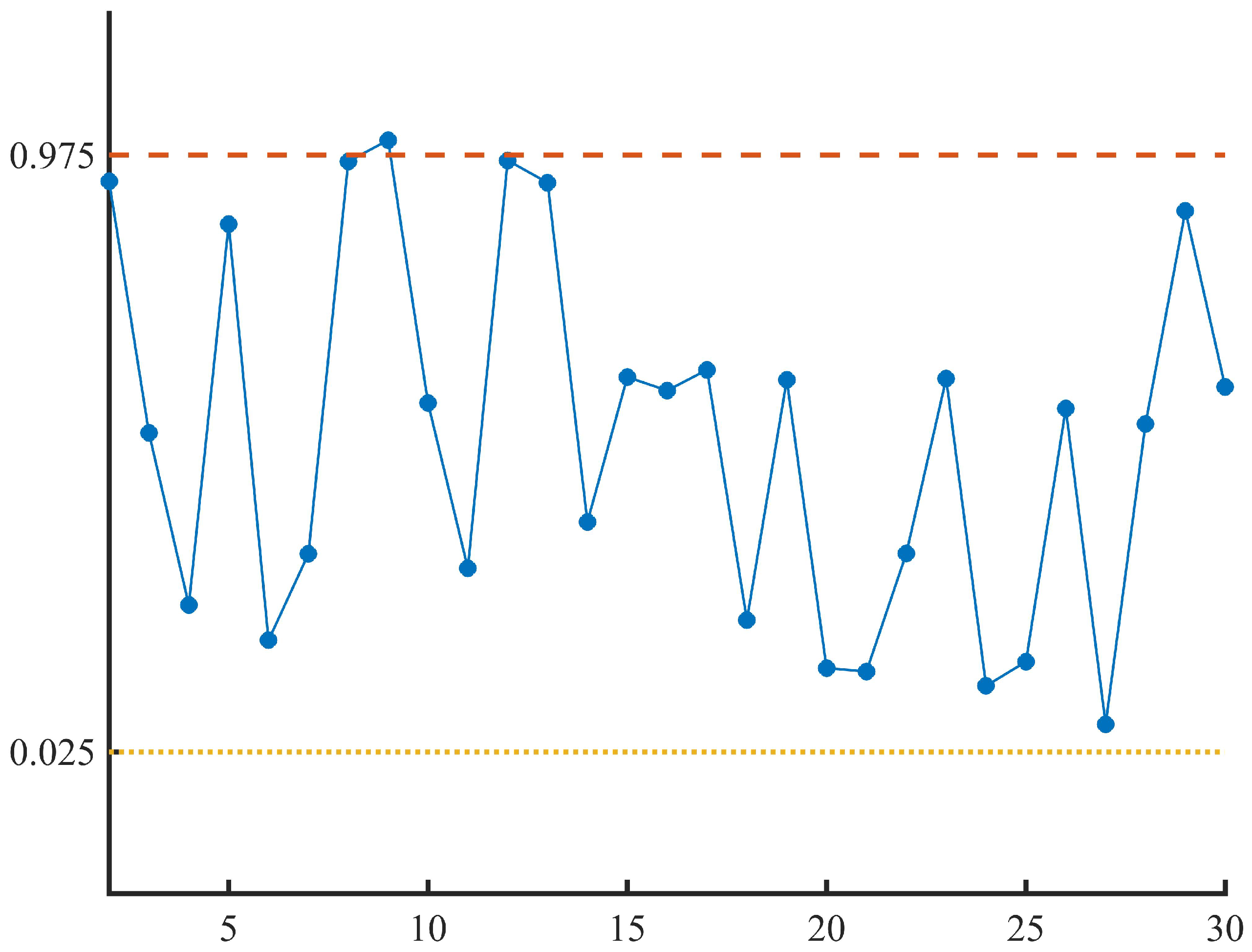
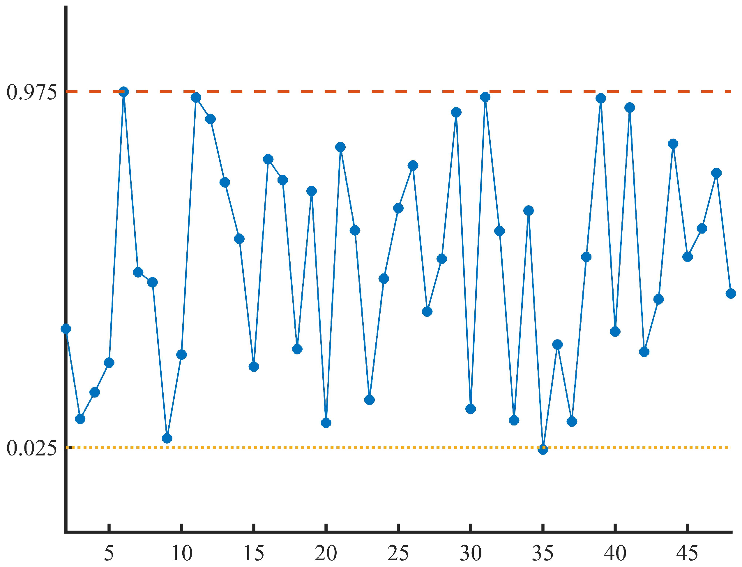
4.3. Uncertain Hypothesis Test

After obtaining the estimated multifactor uncertain mean reversion stock model (11), we substitute the observational data and the estimated parameters into

$${\epsilon }_2(m,a,{\sigma }_1,{\sigma }_2),{\epsilon }_3(m,a,{\sigma }_1,{\sigma }_2),\cdots ,{\epsilon }_{126}(m,a,{\sigma }_1,{\sigma }_2).$$

Then, we can generate 125 residuals ${\epsilon }_2,{\epsilon }_3,\cdots ,{\epsilon }_{126}$, which are depicted in Figure 6.

For the sake of assessing the suitability of the estimated multifactor uncertain mean reversion stock model (11) for representing the data shown in Table 3 and Figure 5, it follows from the work of Ye and Liu [30] that we only need to examine whether the linear uncertainty distribution $\mathcal{L}(0,1)$ adequately describes the residuals ${\epsilon }_2,{\epsilon }_3,\cdots ,{\epsilon }_{126}$. Assume the significance level takes the value of $\alpha =0.05$. Then, we have $\alpha \times 125=6.25$ and the test is

$$\begin{array}{cc}\hfill W=\left\{\right(z_2,z_3,& \cdots ,z_{126}):\mathrm{t}\mathrm{h}\mathrm{e}\mathrm{r}\mathrm{e} \mathrm{a}\mathrm{r}\mathrm{e} \mathrm{a}\mathrm{t} \mathrm{l}\mathrm{e}\mathrm{a}\mathrm{s}\mathrm{t} 7 \mathrm{o}\mathrm{f} \mathrm{i}\mathrm{n}\mathrm{d}\mathrm{e}\mathrm{x}\mathrm{e}\mathrm{s} i’\mathrm{s} \mathrm{w}\mathrm{i}\mathrm{t}\mathrm{h} 2\le i\le 126\hfill \\ \hfill & \mathrm{s}\mathrm{u}\mathrm{c}\mathrm{h} \mathrm{t}\mathrm{h}\mathrm{a}\mathrm{t} z_i<0.025 \mathrm{o}\mathrm{r} z_i>0.975\}.\hfill \end{array}$$

As depicted in Figure 6, it is evident that only

$${\epsilon }_8,{\epsilon }_{19},{\epsilon }_{72}\notin [0.025,0.975].$$

Consequently, we can infer that

$$({\epsilon }_2,{\epsilon }_3,\cdots ,{\epsilon }_{126})\notin W.$$

This strongly supports the conclusion that the linear uncertainty distribution $\mathcal{L}(0,1)$ can adequately describe the residuals ${\epsilon }_2,{\epsilon }_3,\cdots ,{\epsilon }_{126}$. Thus, the estimated multifactor uncertain mean reversion stock model (11) serves as an excellent fit for JD.com’s stock prices.

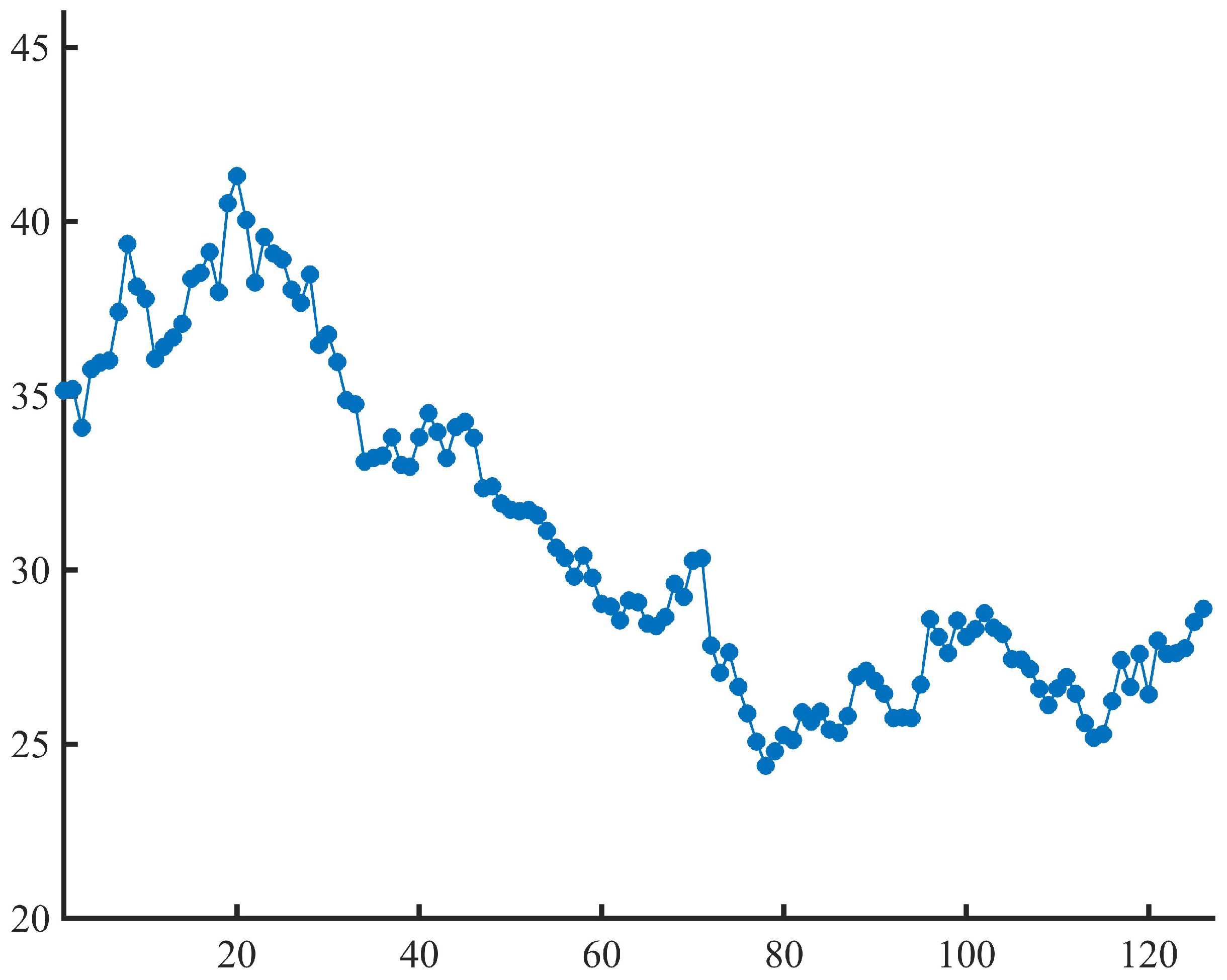
4.4. Stock Price Forecasting

Based on the suitability of the determined multifactor uncertain mean reversion stock model (11), we use the model to forecast JD.com’s stock prices in 2024. Here, we select the closing prices of JD.com’s stock on all trading days between 1 January 2024 and 15 May 2024 as the real data (94 data points in total).

Let us denote the trading days spanning from 1 January 2024 to 15 May 2024 as $t=127,128,\cdots ,220$. Then, JD.com’s stock prices and actual closing prices for this period can be denoted as

$$X_t,t=127,128,\cdots ,220,$$

(12)

and

$$x_t,t=127,128,\cdots ,220,$$

respectively. For each index i with $127\le i\le 220$, the closing price of JD.com’s stock on the ith trading day can be forecasted by solving the following multifactor uncertain differential equation

$$\left\{\begin{array}{cc}{\displaystyle \mathrm{d}{X}_t=\left(6.2177-0.2086X_t\right)\mathrm{d}t+0.0001\mathrm{d}{C}_{1t}+0.0422X_t\mathrm{d}{C}_{2t},}\hfill & \\ {\displaystyle X_{i-1}=x_{i-1},}\hfill \end{array}\right.$$

which can be denoted as ${\widehat{X}}_i$. The forecast values of the closing price of JD.com’s stock on the ith trading day is the expected value of ${\widehat{X}}_i$, i.e.,

$${\widehat{\mu }}_i=E\left[{\widehat{X}}_i\right].$$

By implementing the above process, we can obtain the forecast values of JD.com’s stock prices from 1 January 2024 to 15 May 2024 as follows:

$${\widehat{\mu }}_{127},{\widehat{\mu }}_{128},\cdots ,{\widehat{\mu }}_{220}.$$

As indicated in Figure 7, the comparison between the real data on JD.com’s stock prices (depicted as blue points) and the forecast values (represented by red points) reveals a remarkable degree of consistency. The forecast values align closely with the real data, which underlines the accuracy of our method. In essence, the efficacy of the proposed method is unequivocally demonstrated by the compelling visual evidence in Figure 7.

5. Conclusions

In order to address the challenge of estimating the unknown parameters within multifactor uncertain differential equations based on the framework of uncertainty theory in multi-source noise environments, this paper innovatively introduced the least-squares estimation method.

Specifically, this paper constructed a statistical invariant with a symmetric uncertainty distribution and determined specific parameters by minimizing the distance between the population distribution and the empirical distribution of the statistical invariant. After introducing the method, this paper also provided two numerical examples to help readers better understand the practical operation and effectiveness of this method. Finally, this paper presented a case study focused on applying the least-squares estimation method in modeling and forecasting JD.com’s stock prices to demonstrate the advantages of this approach.

In the future, researchers can further apply the parameter estimation method based on multifactor uncertain differential equations to classical scenarios such as finance and the economy for system modeling, market prediction, and empirical research. In addition, researchers can consider the estimation of initial values and initial times of multifactor uncertain differential equations, along with other related research in statistical inference of multifactor uncertain differential equations.

References

1. Kolmogorov, A. Grundbegriffe der Wahrscheinlichkeitsrechnung; Springer: Berlin, Germany, 1933. [Google Scholar]
2. Liu, B. Uncertainty Theory, 2nd ed.; Springer: Berlin, Germany, 2007. [Google Scholar]
3. Yao, K. Uncertain Differential Equations; Springer: Berlin, Germany, 2016. [Google Scholar]
4. Zhu, Y. Uncertain Optimal Control; Springer: Singapore, 2019. [Google Scholar]
5. Yao, K. Uncertain Renewal Processes; Springer: Singapore, 2019. [Google Scholar]
6. Zhang, B.; Peng, J. Uncertain Graph and Network Optimization; Springer: Singapore, 2022. [Google Scholar]
7. Liu, B. Some research problems in uncertainty theory. J. Uncertain Syst. 2009, 3, 3–10. [Google Scholar]
8. Liu, B. Fuzzy process, hybrid process and uncertain process. J. Uncertain Syst. 2008, 2, 3–16. [Google Scholar]
9. Yang, L.; Liu, Y. Solution method and parameter estimation of uncertain partial differential equation with application to China’s population. Fuzzy Optim. Decis. Mak. 2024, 23, 155–177. [Google Scholar] [CrossRef]
10. Ye, T.; Liu, B. Uncertain significance test for regression coefficients with application to regional economic analysis. Commun.-Stat.-Theory Methods 2023, 52, 7271–7288. [Google Scholar] [CrossRef]
11. Jia, L.; Li, D.; Guo, F.; Zhang, B. Knock-in options of mean-reverting stock model with floating interest rate in uncertain environment. Int. J. Gen. Syst. 2024, 53, 331–351. [Google Scholar] [CrossRef]
12. Liu, Z. Uncertain growth model for the cumulative number of COVID-19 infections in China. Fuzzy Optim. Decis. Mak. 2021, 20, 229–242. [Google Scholar] [CrossRef]
13. Yang, L. Analysis of death toll from COVID-19 in China with uncertain time series and uncertain regression analysis. J. Uncertain Syst. 2022, 15, 2243007. [Google Scholar] [CrossRef]
14. Ding, C.; Ye, T. Uncertain logistic growth model for confirmed COVID-19 cases in Brazil. J. Uncertain Syst. 2022, 15, 2243008. [Google Scholar] [CrossRef]
15. Xie, J.; Lio, W. Uncertain nonlinear time series analysis with applications to motion analysis and epidemic spreading. Fuzzy Optim. Decis. Mak. 2024, 23, 279–294. [Google Scholar] [CrossRef]
16. Yao, K.; Liu, B. Parameter estimation in uncertain differential equations. Fuzzy Optim. Decis. Mak. 2020, 19, 1–12. [Google Scholar] [CrossRef]
17. Liu, Z. Generalized moment estimation for uncertain differential equations. Appl. Math. Comput. 2021, 392, 125724. [Google Scholar] [CrossRef]
18. Sheng, Y.; Yao, K.; Chen, X. Least squares estimation in uncertain differential equations. IEEE Trans. Fuzzy Syst. 2020, 28, 2651–2655. [Google Scholar] [CrossRef]
19. Yang, X.; Liu, Y.H.; Park, G. Parameter estimation of uncertain differential equation with application to financial market. Chaos Solitons Fract. 2020, 139, 110026. [Google Scholar] [CrossRef]
20. Liu, Y.; Liu, B. Estimating unknown parameters in uncertain differential equation by maximum likelihood estimation. Softw. Comput. 2022, 26, 2773–2780. [Google Scholar] [CrossRef]
21. Liu, Y.; Liu, B. Residual analysis and parameter estimation of uncertain differential equations. Fuzzy Optim. Decis. Mak. 2022, 21, 513–530. [Google Scholar] [CrossRef]
22. Liu, Y.; Liu, B. A modified uncertain maximum likelihood estimation with applications in uncertain statistics. Commun.-Stat.-Theory Methods 2023, 1–22. [Google Scholar] [CrossRef]
23. Liu, Y.; Liu, B. Estimation of uncertainty distribution function by the principle of least squares. Commun.-Stat.-Theory Methods 2023, 1–18. [Google Scholar] [CrossRef]
24. Lio, W.; Liu, B. Initial value estimation of uncertain differential equations and zero-day of COVID-19 spread in China. Fuzzy Optim. Decis. Mak. 2021, 20, 177–188. [Google Scholar] [CrossRef]
25. Mehrdoust, F.; Noorani, I.; Xu, W. Uncertain energy model for electricity and gas futures with application in spark-spread option price. Fuzzy Optim. Decis. Mak. 2023, 22, 123–148. [Google Scholar] [CrossRef]
26. Yang, X.; Ke, H. Uncertain interest rate model for Shanghai interbank offered rate and pricing of American swaption. Fuzzy Optim. Decis. Mak. 2023, 22, 447–462. [Google Scholar] [CrossRef]
27. Liu, Z.; Li, Y. Pricing and valuation of carbon swap in uncertain finance market. Fuzzy Optim. Decis. Mak. 2024, 1–18. [Google Scholar] [CrossRef]
28. Ye, T.; Zheng, H. Analysis of birth rates in China with uncertain statistics. J. Intell. Fuzzy Syst. 2023, 44, 10621–10632. [Google Scholar] [CrossRef]
29. Li, S.; Peng, J.; Zhang, B. Multifactor uncertain differential equation. J. Uncertain. Anal. Appl. 2015, 3, 7. [Google Scholar] [CrossRef]
30. Ye, T.; Liu, B. Uncertain hypothesis test for uncertain differential equations. Fuzzy Optim. Decis. Mak. 2023, 22, 195–211. [Google Scholar] [CrossRef]
31. Poterba, J.; Summers, L. Mean reversion in stock prices: Evidence and implications. J. Financ. Econ. 1988, 22, 27–59. [Google Scholar] [CrossRef]
32. Peng, J.; Yao, K. A new option pricing model for stocks in uncertainty markets. Int. J. Oper. Res. 2011, 8, 18–26. [Google Scholar]
33. Sun, Y.; Su, T. Mean-reverting stock model with floating interest rate in uncertain environment. Fuzzy Optim. Decis. Mak. 2017, 16, 235–255. [Google Scholar] [CrossRef]
Figure 1. Observational data of Example 1.
Symmetry 16 00904 g001
Figure 2. Plot of the residuals of the estimated multifactor linear uncertain differential Equation (7) in Example 1.
Symmetry 16 00904 g002
Figure 3. Observational data of Example 2.
Symmetry 16 00904 g003
Figure 4. Plot of the residuals of the estimated multifactor exponential uncertain differential Equation (8) in Example 2.
Symmetry 16 00904 g004
Figure 5. The closing price data (unit: US dollars) of JD.com’s American depositary shares on each trading day from 1 July 2023 to 31 December 2023, as reported by Nasdaq https://www.nasdaq.com/market-activity/stocks/jd/historical (accessed on 17 May 2024).
Symmetry 16 00904 g005
Figure 6. Plot of the residuals of the multifactor uncertain mean reversion stock model (11).
Symmetry 16 00904 g006
Figure 7. The real data and forecast values of JD.com’s stock prices from 1 January 2024 to 15 May 2024.
Symmetry 16 00904 g007