Article

Comparing the Numerical Solution of Fractional Glucose–Insulin Systems Using Generalized Euler Method in Sense of Caputo, Caputo–Fabrizio and Atangana–Baleanu

Mathematics Department, Faculty of Science, Northern Border University, Arar 73222, Saudi Arabia
Symmetry 2024, 16(7), 919; https://doi.org/10.3390/sym16070919
Submission received: 12 June 2024 / Revised: 10 July 2024 / Accepted: 15 July 2024 / Published: 18 July 2024

Abstract

:
The purpose of this paper is to present a fractional nonlinear mathematical model with beta-cell kinetics and glucose–insulin feedback in order to describe changes in plasma glucose levels and insulin levels over time that may be associated with changes in beta-cell kinetics. We discuss the solution to the problem with respect to its existence, uniqueness, non-negativity, and boundedness. Using three different fractional derivative operators, the proposed model is examined. To approximate fractional-order systems, we use an efficient numerical Euler method in Caputo, Caputo–Fabrizio, and Atangana–Baleanu sense. Several asymptomatic behaviors are observed in the proposed models based on these three operators. These behaviors do not appear in integer-order derivative models. These behaviors are essential for understanding fractional-order systems dynamics. Our results provide insight into fractional-order systems dynamics. These operators analyze local and global stability and Hyers–Ulam stability. Furthermore, the numerical solutions for the proposed model are simulated using the three methods.

1. Introduction

It is well known that the secretion of insulin and the biological effectiveness of insulin during periods of glucose loading are strongly influenced by (i) the number and functional capacity of pancreatic beta cells, as well as (ii) peripheral resistance to insulin action during glucose loading. Diabetes mellitus is characterized by a slowing of insulin release, combined with a diminished secretory response to insulin, attributable to peripheral resistance to insulin. These factors can contribute to the development of glucose intolerance, the main symptom of the disease. Several mathematical models have been proposed over the years as a means of explaining the relationship between insulin and glucose concentrations in plasma in response to a load of glucose in the body.
There have been numerous mathematical models proposed over the years, but the most recent is proposed by Ackerman et al. [1], which describes the glucose tolerance test using two autonomous first-order differential equations.
d x d t = a 1 y a 2 x + c 1 ,
d y d t = a 3 y a 4 x + c 2 .
In this case, x ( t ) and y ( t ) are the insulin and glucose levels, respectively, at a given point in time. In x ( t ) and y ( t ) , the concentration differences between fasting levels are represented. As shown in the equation above, a 1 y represents the net increase in insulin due to glucose exposure, a 2 x represents the rate of insulin removal, a 3 y represents the rate of glucose removal independent of insulin, and a 4 x represents the rate of glucose reduction due to insulin. For both x and y, c 1 and c 2 are positive constants corresponding to zero order rates of increase. As early as the 1970s, Molnar et al. [2] developed a model that incorporated a modified form of Equation (2) and another mathematical equation that was derived directly from Equations (1) and (2). A model system comprised of three nonlinear differential equations was developed by Bajaj and Rao [3,4] that used the following formulation to account for the kinetic properties of beta cells within the glucose–insulin feedback system:
d x d t = S 1 y S 2 x + c 1 , d y d t = S 3 N z S 4 x + c 2 , d z d t = S 5 y ( T z ) + S 6 z ( T z ) S 7 z .
As can be seen in Table 1, there are a number of parameters associated with the model (3).
Overall, a negative feedback loop between β -cells and the body’s basal insulin and glucose concentrations has been established [5,6]. The model proposed by Bajaj and Roa in [3] addressed the role of β -cells in regulating plasma insulin levels by Lenbury et al. [7]. The rates S 1 , S 2 , c 1 are determined by the density of the beta cells. This concept of fractional calculus plays a significant role in many branches of mathematics in addition to being important when attempting to model real-world problems [8,9,10,11,12,13,14,15,16,17,18,19,20,21,22,23,24,25,26]. For further information regarding the use of fractional-order differential equations in biological studies, please refer to [27,28,29,30,31,32,33,34,35,36,37,38,39,40]. There are a variety of fractional derivatives with nonsingular kernels proposed for describing nonlocal systems in a more accurate and practical way. These derivatives have been compared to fractional derivatives. Based on the type of function specified by exponentials and Mittag–Leflers [36,37], there are two very plausible possibilities among the existing definitions.
This study presents a fractional nonlinear mathematical model incorporating beta-cell kinetics and a glucose–insulin feedback system that allows us to describe plasma glucose and insulin level changes over time. The model solution is discussed in terms of its existence, uniqueness, non-negativity, and boundedness. To approximate fractional-order systems, we employ an efficient numerical Euler method in Caputo, Caputo–Fabrizio, and Atangana–Baleanu. We investigate steady-state stability at the local and global levels. In comparison to other existing methods, the proposed approach is easier to implement and more efficient due to its properties. Based on the simulation, it is confirmed that the modified model with three different fractional operators exhibits distinct asymptomatic behaviors that are not found in the integer-order model. Fractional derivatives account for the system’s history, incorporating past states into current dynamics. This allows the model to capture long-term dependencies and the cumulative effect of glucose and insulin levels over time, which is not possible with integer-order models. The fractional-order model allows greater flexibility in fitting experimental data. By adjusting the order of the fractional derivatives, the model can better match the observed behavior of glucose and insulin levels. This captures subtleties integer-order models might miss. Fractional operators are inherently nonlocal, meaning they consider the entire history of a function rather than just its local behavior. This nonlocality provides a more accurate description of the glucose–insulin feedback mechanism, which is influenced by past fluctuations in glucose and insulin concentrations.
This article addresses the development of a comprehensive mathematical model that accurately represents the dynamic interactions between insulin and glucose levels in the body. It incorporates the kinetics of beta cells. Traditional integer-order models cannot capture biological systems’ complex, nonlocal, and memory-dependent nature. This study aims to overcome these limitations by employing fractional calculus to develop such a nonlinear mathematical model. The challenge lies in ensuring model accuracy, stability, and practicality while incorporating fractional derivatives. In addition, it lies in providing a numerical method that is both efficient and easy to implement. This approach is expected to offer more realistic insights into the glucose–insulin feedback system and better match quantitative observations to existing models.

2. Preliminaries and Definitions

In [35], the classic Caputo fractional derivative is presented. However, the classical version may not work properly in nonlocal dynamics due to its singular kernel. Many new derivatives have been introduced to overcome this drawback, such as Caputo–Fabrizio ( CF ) [36] and Mittag-Leffler ( AB ) [37]. In the CF derivative, the exponential function is used as the kernel, while in the AB derivative, the ML function is used. Here are the definitions of the classic Caputo operator, CF , and AB .
Definition 1 
([35]). For h : [ a , b ] R , n 1 < ρ 1 n and n N , the Caputo fractional derivative is defined as follows:
  a C D t ρ 1 h ( t ) = 1 Γ ( n ρ 1 ) a t h ( n ) ( γ ) ( t γ ) n ρ 1 1 d γ .
The Caputo derivative is a generalization of the Riemann–Liouville fractional derivative and is used to describe processes that are locally continuous and globally smooth. Additionally, the fractional integral is given as follows:
  a C I t ρ 1 h ( t ) = 1 Γ ( ρ 1 ) a t h ( γ ) ( t γ ) ρ 1 1 d γ .
Model (3) can be written in sense of Caputo as:
  a C D t ρ 1 x = S 1 y S 2 x + c 1 ,   a C D t ρ 1 y = S 3 N z S 4 x + c 2 ,   a C D t ρ 1 z = S 5 y ( T z ) + S 6 z ( T z ) S 7 z .
Definition 2 
([36]). For h H 1 ( a , b ) and 0 < ρ 1 < 1 , the Caputo–Fabrizio derivative is defined as follows:
  a CF D t ρ 1 h ( t ) = 1 1 ρ 1 a t d h ( γ ) d γ e β ( t γ ) d γ ,
where β = ρ 1 1 ρ 1 . The corresponding fractional integral is CF and has the following properties:
  a CF I t ρ 1 h ( t ) = ( 1 ρ 1 ) h ( t ) + ρ 1 a t h ( γ ) d γ .
Model (3) can be written in sense of Caputo as:
  a CF D t ρ 1 x = S 1 y S 2 x + c 1 ,   a CF D t ρ 1 y = S 3 N z S 4 x + c 2 ,   a CF D t ρ 1 z = S 5 y ( T z ) + S 6 z ( T z ) S 7 z .
Definition 3 
([37]). For h H 1 ( a , b ) and 0 < ρ 1 < 1 , the AB derivative of order ρ 1 is
  a AB D t ρ 1 h ( t ) = B ( ρ 1 ) 1 ρ 1 a t d h ( γ ) d γ E ρ 1 β ( t γ ) ρ 1 d γ ,
where B ( ρ 1 ) with B ( 0 ) = B ( 1 ) = 1 denotes the normalization function, β = ρ 1 1 ρ 1 and E ρ 1 is the ML function. Also, the corresponding AB fractional integral is
  AB   a I t ρ 1 h ( t ) = 1 ρ 1 B ( ρ 1 ) h ( t ) + ρ 1 B ( ρ 1 ) Γ ( ρ 1 ) a t h ( γ ) ( t γ ) ρ 1 1 d γ .
Model (3) can be written in sense of Caputo as:
  a AB D t ρ 1 x = S 1 y S 2 x + c 1 ,   a AB D t ρ 1 y = S 3 N z S 4 x + c 2 ,   a AB D t ρ 1 z = S 5 y ( T z ) + S 6 z ( T z ) S 7 z .
According to the following equation, the differentiation operators discussed above have a useful relationship to their corresponding fractional integrals
  a C I t ρ 1   a C D t ρ 1 h ( t ) =   a CF I t ρ 1   a CF D t ρ 1 h ( t ) =   AB   a I t ρ 1   AB   a D t ρ 1 h ( t ) = h ( t ) h ( a ) .
Each of the Caputo, CF, and AB fractional derivatives has its own advantages and disadvantages. The Caputo fractional derivative is widely used for its simplicity and ease of interpretation, while the CF fractional derivative offers better numerical stability and accuracy. The AB fractional derivative provides a more flexible and generalized framework for fractional calculus, but it can be computationally demanding and complex to implement.

3. Euler Method Involving Caputo, Caputo–Fabrizio, and Atangana–Baleanu Operators

There are several numerical methods presented in this section for solving the models (5), (7) and (9) using the fractional Euler method (10) that employs the Caputo, Caputo–Fabrizio, and Atangana–Baleanu operators. As a result of applying one of the fractional integral operators (4), (6), or (8) to Equation (4), we obtain:
z ( t ) = z 0 +   0 I t ρ 1 g ( z ( t ) ) , 0 < t < b < ,
  0 I t ρ 1 indicates the integral operator corresponding to the fractional derivatives of Caputo, CF and AB . The numerical scheme is designed based on a uniform grid on [ 0 , b ] with time steps of h = b 0 N . We will use z k to approximate z ( t ) at t = t k , where t k = 0 + k h and k = 0 , 1 , N . By discretizing Equation (10) using the Euler method [34], we determine the following formulas for Caputo, CF and AB .
z k + 1 = z 0 + h ρ 1 Γ ( ρ 1 + 1 ) i = 0 k ω k + 1 , i g z i , k = 0 , , N 1 ,
z k + 1 = z 0 + ( 1 ρ 1 ) g z k + 1 + ρ 1 h i = 0 k g z i , k = 0 , , N 1 ,
z k + 1 = z 0 + 1 ρ 1 B ( ρ 1 ) g z k + 1 + h ρ 1 B ( ρ 1 ) Γ ( ρ 1 ) i = 0 k ω k + 1 , i g z i , k = 0 , , N 1 ,
where ω k + 1 , j = ( k + 1 i ) ρ 1 ( k j ) ρ 1 , j = 0 , , k . According to Equation (11), the discrete form of Equation (5) is
x n + 1 = x 0 + h ρ 1 Γ ( ρ 1 + 1 ) j = 0 n ω k + 1 , j [ S 1 y j S 2 x j + c 1 ] , y n + 1 = y 0 + h ρ 1 Γ ( ρ 1 + 1 ) j = 0 n ω k + 1 , j S 3 N z j S 4 x j + c 2 , z n + 1 = z 0 + h ρ 1 Γ ( ρ 1 + 1 ) j = 0 n ω k + 1 , j S 5 y j ( T z j ) + S 6 z j ( T z j ) S 7 z j .
In terms of discrete form, Equation (7) can be expressed as follows using Equation (12):
x n + 1 = x 0 + ( 1 ρ 1 ) [ S 1 y k + 1 S 2 x k + 1 + c 1 ] + ρ 1 h j = 0 n [ S 1 y j S 2 x j + c 1 ] , y n + 1 = y 0 + ( 1 ρ 1 ) S 3 N z k + 1 S 4 x k + 1 + c 2 + ρ 1 h j = 0 n S 3 N z j S 4 x j + c 2 , z n + 1 = z 0 + ( 1 ρ 1 ) S 5 y k + 1 ( T z k + 1 ) + S 6 z k + 1 ( T z k + 1 ) S 7 z k + 1 + ρ 1 h j = 0 n S 5 y j ( T z j ) + S 6 z j ( T z j ) S 7 z j .
Equation (9) can be expressed in discrete form according to Equation (13)
x n + 1 = x 0 + 1 ρ 1 B ( ρ 1 ) [ S 1 y k + 1 S 2 x k + 1 + c 1 ] + h ρ 1 B ( ρ 1 ) Γ ( ρ 1 ) j = 0 n ω k + 1 , j [ S 1 y j S 2 x j + c 1 ] , y n + 1 = y 0 + 1 ρ 1 B ( ρ 1 ) S 3 N z k + 1 S 4 x k + 1 + c 2 + h ρ 1 B ( ρ 1 ) Γ ( ρ 1 ) j = 0 n ω k + 1 , j S 3 N z j S 4 x j + c 2 , z n + 1 = z 0 + 1 ρ 1 B ( ρ 1 ) S 5 y k + 1 ( T z k + 1 ) + S 6 z k + 1 ( T z k + 1 ) S 7 z k + 1 + h ρ 1 B ( ρ 1 ) Γ ( ρ 1 ) j = 0 n ω k + 1 , j S 5 y j ( T z j ) + S 6 z j ( T z j ) S 7 z j .
This paper enhances the understanding of discrete approaches for solving fractional-order nonlinear differential equations, facilitating more informed decisions in modeling and simulation. The comparative analysis underscores the importance of choosing the right numerical method for solving fractional-order nonlinear differential equations. While the Euler method offers simplicity and speed, the predictor-corrector method provides superior accuracy and stability, making it suitable for more complex and precise applications. Researchers can leverage this analysis to optimize their numerical simulations, achieving reliable and efficient solutions tailored to their specific needs.
By conducting a detailed comparative analysis of the Euler method and the predictor-corrector method [41], the paper can better highlight the contributions and practical implications of the proposed approach. This analysis will provide a comprehensive understanding of the strengths and limitations of different numerical methods for solving fractional-order systems, guiding researchers in choosing the most suitable method for their specific needs.

4. Properties of the Solutions

4.1. Existence, Uniqueness, Non-Negativity, and Boundedness

As can be seen in the following representation, the fractional-order system (14) is as follows:
  a * D t ρ 1 W = F ( W ) , t [ 0 , T ] , 0 < ρ 1 1 , W ( 0 ) = W 0 ,
where   a * D t ρ 1 is one of the Caputo, CF and AB fractional derivatives, and
W = x y z , W 0 = x 0 y 0 z 0 , F ( W ) = S 1 y S 2 x + c 1 S 3 N z S 4 x + c 2 S 5 y ( T z ) + S 6 z ( T z ) S 7 z .
Define the supremum norm as
N = sup t [ 0 , T ] | N | .
Then the norm of the matrix M = [ m i j [ t ] ] is defined by
M = i j sup t [ 0 , T ] [ m i j [ t ] ] .
It is now important to establish the existence and the uniqueness of the solutions of (2) in the region Ω × ( 0 , T ] with respect to
Ω = { ( x , y , z ) R 3 : max ( | x | , | y | , | z | ) η } .
Theorem 1. 
In the region Ω, it is sufficient to maintain that fractional-order systems’ solutions (14) will exist and be unique if and only if W ( 0 ) = W 0 exists in the region Ω.
0 < T ρ 1 Γ ( ρ 1 + 1 ) m a x { S 2 + S 4 , S 1 + S 5 ( T + η ) , ( S 5 + 2 S 6 ) η + S 6 T + S 7 + S 3 N } < 1
Proof. 
The following is the solution to system (4)
W = W 0 + 1 Γ ( ρ 1 ) 0 t ( t s ) ρ 1 1 F ( W ( s ) ) d s = G ( W ) .
So
G ( W 1 ) G ( W 2 ) = 1 Γ ( ρ 1 ) 0 t ( t s ) ρ 1 1 ( F ( W 1 ( s ) ) F ( W 2 ( s ) ) ) d s .
Consequently, we are left with the following inequality as a result
| G ( W 1 ) G ( W 2 ) | 1 Γ ( ρ 1 ) 0 t ( t s ) ρ 1 1 ( F ( W 1 ( s ) ) F ( W 2 ( s ) ) ) d s .
The following inequality is obtained after some calculations
G ( W 1 ) G ( W 2 )   T ρ 1 Γ ( ρ 1 + 1 ) m a x { S 2 + S 4 , S 1 + S 5 ( T + η ) , ( S 5 + 2 S 6 ) η + S 6 T + S 7 + S 3 N ) } W 1 W 2   K W 1 W 2 ,
where
K = T ρ 1 Γ ( ρ 1 + 1 ) m a x { S 2 + S 4 , S 1 + S 5 ( T + η ) , ( S 5 + 2 S 6 ) η + S 6 T + S 7 + S 3 N } .
Consequently, if 0 < K < 1 , W = G ( W ) represents a contraction mapping. □
Theorem 2. 
Considering c 2 S 4 η as a means to return the solutions to the system (14), which start at R + 3 , are non-negative.
Proof. 
Negative values are not considered to be physically meaningful, so they are not considered when attempting to solve problems in biology. Positive bounded solutions are the most realistic and biologically relevant solutions, so they are often sought out when trying to solve biological problems. As a result, this leads to
  a * D t ρ 1 x | x = 0 = S 1 y + c 1 0 ,   a * D t ρ 1 y | y = 0 = S 3 N z S 4 x + c 2 c 2 S 4 η 0 ,   a * D t ρ 1 z | z = 0 = S 5 y ( T z ) + S 6 z ( T z ) S 7 z = S 5 y T 0 ,
It is concluded from Lemmas 5 and 6 under [42] that the Caputo fractional model (14) solutions can be classified as semi-positive under the assumptions. □
Theorem 3. 
Solutions to model (2), which begin in R + 3 , are uniformly bounded by
Ω = ( x , y , z ) R + 3 : N δ η + S 1 η + S 5 T η + c 1 + c 2 + S 3 N z * δ + ε , ε > 0 .
Proof. 
In order to follow the [34] approach, the following method is adopted. In order to understand this equation, take into consideration that N = x + y + z . In that case,
  a * D t ρ 1 N =   a * D t ρ 1 x +   a * D t ρ 1 y +   a * D t ρ 1 z = [ S 4 + S 2 ] x + [ S 1 + S 5 T ] y [ S 7 + S 6 T ] z + c 1 + c 2 + S 3 N z S 5 y z S 6 z 2 .
Therefore, for any δ > 0 , the following is true:
  a * D t ρ 1 N + δ N = [ δ ( S 4 + S 2 ) ] x + [ δ + S 1 + S 5 T ] y + [ δ ( S 7 + S 6 T ) ] z + c 1 + c 2 + S 3 N z S 5 y z S 6 z 2 .
One can choose δ < m i n { S 4 + S 2 , S 7 + S 6 T } . Thus
  a * D t ρ 1 N + δ N δ η + S 1 η + S 5 T η + c 1 + c 2 + S 3 N z * .
It follows from [24], Lemma 9, that we are able to
0 N N ( 0 ) E ρ 1 ( δ ρ 1 ) + r ρ 1 E ρ 1 , ρ 1 + 1 ( δ ρ 1 ) ) .
Here, E q is the Mittag-Leffler function as used by Mittag-Leffler. Based on [42], with reference to Lemma 5 and Corollary 6, one can obtain the following result:
0 N δ η + S 1 η + S 5 T η + c 1 + c 2 + S 3 N z * δ , t
This result leads to the uniform boundedness in the region W for the solution of the model (14). This means that any solution u of the model starting in W will be bounded for all t 0 . Moreover, the solutions will remain bound for all subsequent times. □

4.2. Stability of the Proposed Model Locally and Globally

E * = ( x * , y * , z * ) provides the steady-state value for the system, where
x * = S 4 N + c 1 z * S 5 z * , y * = S 4 S 7 N + ( S 7 c 1 S 5 c 2 ) z * S 5 S 6 z * .
Here z * is the steady-state value satisfied by the cubic equation.
( z * ) 3 + d 1 ( z * ) 2 + d 2 z * + d 3 = 0 ,
where
d 1 = ( S 3 c 1 T S 2 c 1 + S 7 c 1 S 5 c 2 ) S 1 S 2 S 5 S 6 , d 2 = ( S 4 S 7 N T S 7 c 1 + T S 5 c 2 ) S 1 S 2 S 5 S 6 , d 3 = T S 1 S 4 S 7 N S 2 S 5 S 6 .
Consequently, the Jacobian matrix for system (14) at equilibrium can be calculated as follows:
J 1 ( E * ) = S 2 S 1 0 S 4 0 S 3 N / ( z * ) 2 0 S 5 ( T z * ) S 5 y * + S 6 T 2 S 6 z * S 7 .
After the linearized system has been linearized, the characteristic equation P 1 ( λ ) is then solved as follows:
P 1 ( λ ) = a 3 λ 3 + a 2 λ 2 + a 1 λ + a 0 = 0 ,
where
a 0 = S 1 S 4 S 7 S 1 S 4 S 6 T + S 1 S 4 S 5 y * + 2 S 1 S 4 S 6 z * S 2 S 3 S 5 N ( z * T ) ( z * ) 2 a 1 = S 1 S 4 + S 2 S 7 S 2 S 6 T + S 2 S 5 y * + 2 S 2 S 6 z * S 3 S 5 N ( z * T ) ( z * ) 2 , a 2 = S 2 + S 7 + S 5 y * S 6 T + 2 S 6 z * , a 3 = 1 .
Lemma 1. 
A local asymptotic stability exists to the equilibrium point E * = ( x * , y * , z * ) .
Proof. 
The Routh–Hurwitz array for the Jacobian matrix J ( E * ) has been implemented in the following manner:
D 1 ( E * ) = a 3 a 1 a 2 a 0 ( a 1 a 2 a 0 a 3 ) a 2 0 a 0 0 .
It is believed that Routh–Hurwitz conditions [43] hold if you verify that ( a 1 a 2 a 0 a 3 ) a 2 has the same sign as a 1 . It follows that the three eigenvalues have negative real parts. In view of the fact that a 0 > 0 , a 1 > 0 , a 2 > 0 , a 3 > 0 , then ( a 1 a 2 a 0 a 3 ) a 2 > 0 and a 1 a 2 > a 0 a 3 hold. This leads to the equilibrium point being an asymptotic stability point, as per Routh–Hurwitz, and thus fulfilling the Routh–Hurwitz stability standards. □
Based on the results cited in [13], we can conclude that Hopf bifurcation occurs when
| arg γ 1 | = ρ 1 π 2 , | arg γ 2 | = ρ 1 π 2 ,
i.e.,
| 4 Δ tr 2 ( J ) tr ( J ) | = tan ρ 1 π 2 ,
i.e.,
| 4 p 1 p 2 p 4 + ( p 1 + p 2 + p 4 ) 2 p 1 + p 2 + p 4 | = tan ρ 1 π 2 .

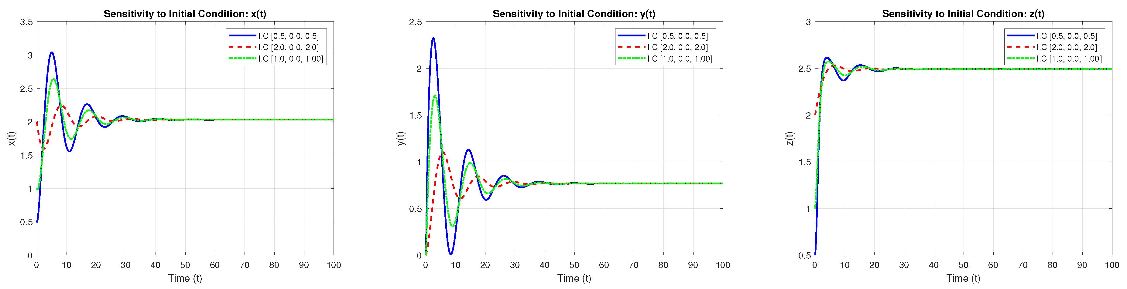
4.3. Sensitivity to Initial Values

This section discusses the sensitivity of fractional glucose–insulin systems to the initial values they are given. Time plots have been taken for three sets of initial conditions: (0.5, 0, 0.5), (2, 0, 2), (1, 0, 1). Sensitivity to initial values implies that changes in the initial values cause fluctuations that are initially negligible, but quickly build up, as shown in Figure 1. The sensitivity of fractional glucose–insulin systems to initial values is a critical aspect that influences their dynamic behavior. By examining the time plots for different initial conditions, we observe that even small changes can lead to substantial differences in system trajectories. This sensitivity highlights the importance of accurate initial condition assessment and tailored interventions in managing glucose–insulin dynamics effectively.

5. Hyers-Ulam Stability

Definition 4 
([44,45]). The constant ζ i > 0 must be large for i N 1 3 . Hyers–Ulam stability for model (5) requires that each constant ζ i > 0 meet the following conditions:
| x ( t )   0 I t ρ 1 T 1 ( x ( t ) ) | ζ 1 , | y ( t )   0 I t ρ 1 T 2 ( y ( t ) ) | ζ 2 , | z ( t )   0 I t ρ 1 T 3 ( z ( t ) ) | ζ 3 .
In the model (14), we can formally represent the approximation as x 1 ( t ) , y 1 ( t ) , z 1 ( t ) that satisfies the following conditions:
| x x 1 | v 1 ξ 1 , | y y 1 | v 2 ξ 2 , | z z 1 | v 3 ξ 3 .
Theorem 4. 
The Hyers–Ulam stability condition is satisfied if (16) is true.
Proof. 
| x x 1 | = |   0 I t ρ 1 T 1 ( x ( t ) )   0 I t ρ 1 T 1 ( x 1 ( t ) ) | 1 ρ 1 B ( ρ 1 ) + ρ 1 B ( ρ 1 ) Γ ( ρ 1 ) ξ 1 x x 1 .
Then
| x x 1 | v 1 ξ 1 ,
with
v 1 = 1 Γ ( ρ 1 ) x x 1 , Caputo fractional integral , x x 1 , Caputo Fabrizio fractional , 1 ρ 1 B ( ρ 1 ) + ρ 1 B ( ρ 1 ) Γ ( ρ 1 ) x x 1 , Atangana Baleanu fractional .
Similarly, one obtains
| y y 1 | v 2 ξ 2 ,
with
v 2 = 1 Γ ( ρ 1 ) y y 1 , Caputo fractional fractional , y y 1 , Caputo Fabrizio fractional , 1 ρ 1 B ( ρ 1 ) + ρ 1 B ( ρ 1 ) Γ ( ρ 1 ) x x 1 , Atangana Baleanu fractional .
Similarly, one obtains
| z z 1 | v 3 ξ 3 ,
with
v 3 = 1 Γ ( ρ 1 ) z z 1 , Caputo fractional integral , z z 1 , Caputo Fabrizio fractional , 1 ρ 1 B ( ρ 1 ) + ρ 1 B ( ρ 1 ) Γ ( ρ 1 ) z z 1 , Atangana Baleanu fractional integral .
Hence, the results follow.  □

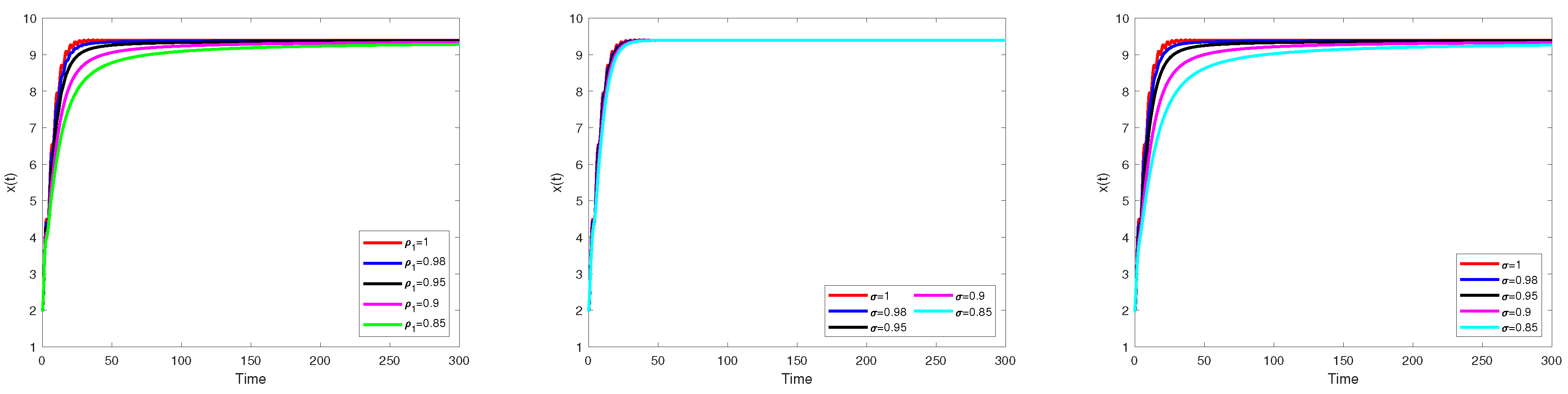
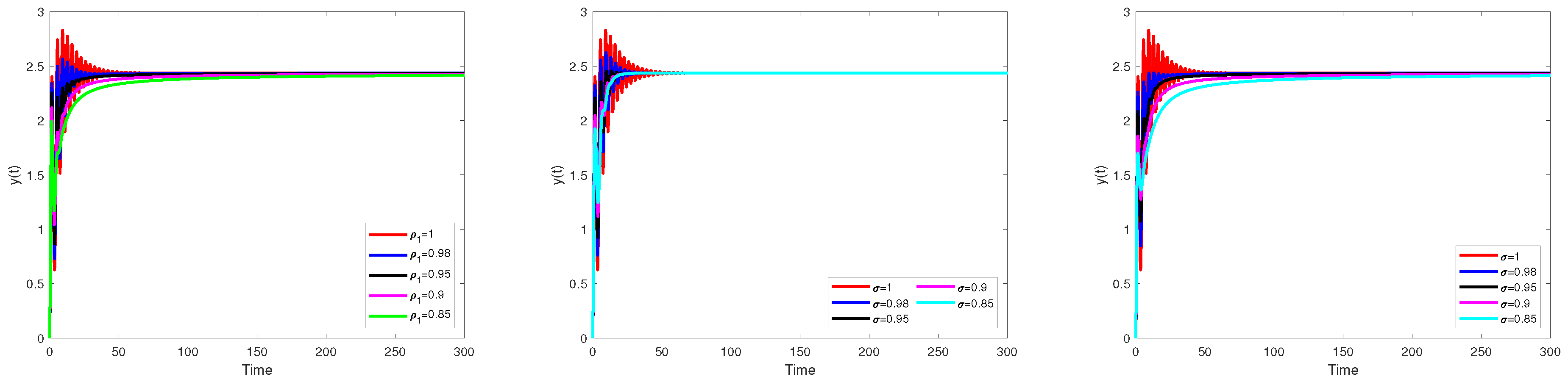
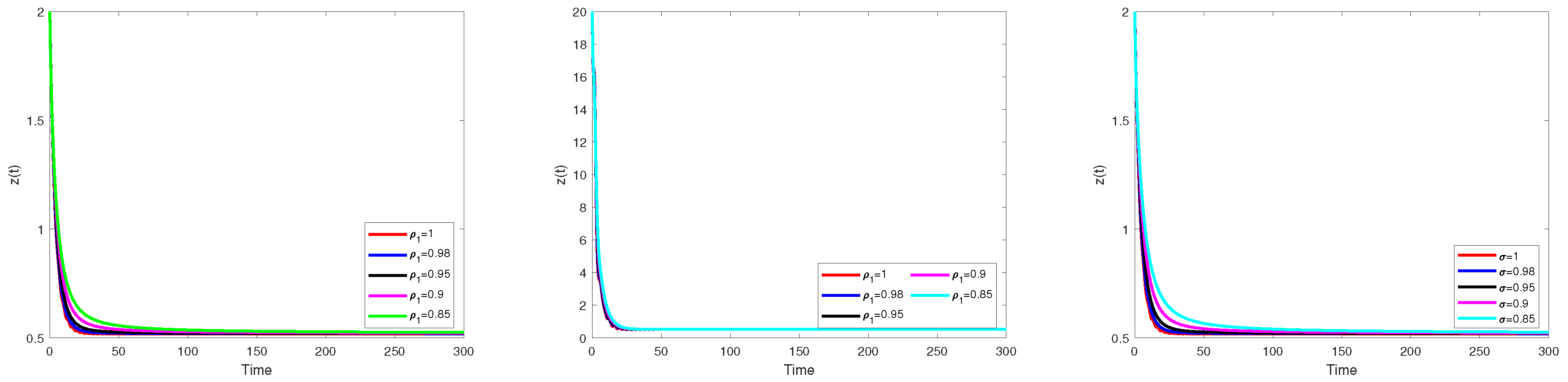
Numerical Simulation

Table 1 provides support for the analytical results as well as assessing the effectiveness of the control strategy for fractional-order values ρ 1 using the Euler method in the sense of the Caputo, Caputo–Fabrizio, and Atangana–Baleanu operators. Consider the following:
Example 1. 
The discretized fractional order we are considering is as follows:
  0 * D t ρ 1 x = 0.79196 y 0.24537 x + 0.37538 ,   0 * D t ρ 1 y = 9.52033 ( 1.4 ) z 2.84575 x + 1.03482 ,   0 * D t ρ 1 z = 0.02139 y ( 1.95 z ) + 0.02747 z ( 1.95 z ) 0.18311 z ,
depending on the initial conditions, E 0 = ( x ( 0 ) , y ( 0 ) , z ( 0 ) ) = ( 2 , 0 , 2 ) .
According to these parameters, E 0 is asymptomatically stable. As predicted, this result leads to the unique disease-free equilibrium E 0 . The comparison of x ( t ) , y ( t ) , and z ( t ) numerical solutions derived using the Euler method in the sense of Caputo, Caputo–Fabrizio, and Atangana–Baleanu operators for different values of ρ 1 = 0.65 , 0.75 , 0.85 , 0.95 , and 1. Using Caputo Euler, Caputo–Fabrizio Euler, and Atangana–Baleanu Euler methods, Figure 2, Figure 3 and Figure 4 compare the numerical solutions to x ( t ) , y ( t ) , and z ( t ) . As a result of these parameters, E 0 appears to be asymptomatic, that is, the solution converges to E 0 . The result is an increase in insulin uptake and an increase in insulin-excitable tissue glucose uptake, which results in a reduction in glucose levels. According to Figure 2, Figure 3 and Figure 4, different values of ρ 1 result in different glucose activities of insulin-excitable tissue glucose uptake and insulin dynamics. Various cases also allow us to plot blood glucose levels, insulin-excitable tissue glucose concentrations, and insulin absorption from excitable tissues over time.

6. Discussion

The proposed method in this manuscript offers a balanced approach, combining accuracy, stability, robustness, and computational efficiency. Its ability to handle fractional-order systems effectively makes it a superior choice for solving complex nonlinear differential equations, particularly in biological modeling. By highlighting these advantages, the manuscript not only underscores the method’s contributions but also provides practical guidance for researchers in selecting the most appropriate numerical techniques for their specific applications. The glucose–insulin system, despite being linear, contains significant and interesting dynamics that are crucial for understanding metabolic regulation and diabetes. These dynamics make it a valuable example for testing numerical solution algorithms and demonstrating the practical applicability of the proposed method. The insights gained from this model can serve as a basis for extending the method to more complex and nonlinear systems. This will enhance its relevance and utility in various fields of biomedical research. By focusing on numerical solution algorithms and using the glucose–insulin system as an illustrative example, the manuscript can provide a comprehensive evaluation of the proposed method. Additionally, extending the discussion to nonlinear systems, such as the Lorenz and Chen systems, will demonstrate the versatility and robustness of the approach. This will make it more relevant and valuable for researchers in various fields. By expanding the method to solve nonlinear chaotic systems like the Lorenz and Chen systems, the authors can demonstrate the versatility and robustness of their proposed numerical solution algorithms. This additional example will strengthen the paper by showing that the method is not limited to linear systems. It can effectively handle nonlinear and chaotic dynamics. Fractional-order systems, characterized by differential equations involving derivatives of non-integer orders, pose unique challenges and opportunities for numerical analysis. In addition to the Euler and predictor–corrector methods [46], numerous other algorithms have been developed to solve fractional-order differential equations. Each method has its strengths and is suited to different types of problems. This section provides an overview of some notable solution algorithms and their applications, highlighting how they compare to the methods discussed in this paper. Given the diversity of solution algorithms, it is essential to choose the method that most effectively fits the specific requirements of the problem at hand. The comparison results highlight the trade-offs between different numerical methods. The Euler method is suitable for quick approximations and scenarios where computational resources are limited. However, for applications requiring high accuracy and stability, such as long-term simulations of the glucose–insulin system, the predictor–corrector method is preferable despite its higher computational cost. For real-time monitoring and control systems, where quick approximations are needed, the Euler method may suffice. However, for detailed studies and accurate biological systems modeling, the predictor–corrector method is recommended. These findings guide researchers in choosing the appropriate method based on their specific needs and constraints. By providing a detailed discussion of the comparison results, the authors can underscore the strengths and limitations of each numerical method, helping readers understand the practical implications of their findings and guiding future research in the field. Local stability ensures the system can withstand small disturbances or noise. For instance, in the glucose–insulin system, local stability means that minor fluctuations in glucose levels or insulin production will not lead to significant deviations from the desired state. Predictability is crucial for maintaining system performance and designing effective control strategies. Global stability implies robustness to large disturbances and varying initial conditions. For the glucose–insulin system, global stability ensures that even significant deviations in glucose levels or insulin production will eventually stabilize to the desired state. This robustness is essential for ensuring the long-term health and functionality of the biological system, making it resilient to unexpected changes and varying initial conditions. By analyzing both local and global stability, we gain a comprehensive understanding of system behavior. Local stability provides insights into the system’s response to minor disturbances, while global stability guarantees robustness against significant deviations. Together, these stability analyses demonstrate the effectiveness and reliability of the proposed fractional-order glucose–insulin model in maintaining stable plasma glucose and insulin levels under various conditions. Figure 2, Figure 3 and Figure 4 show the trajectories of the state variables x(t), y(t), and z(t) starting from initial conditions near E * . As seen in the figure, all state variables converge to their respective equilibrium values x * , y * , and z * over time. Numerical simulations support Lemma 1. The convergence of the state variables to the equilibrium point E * , as demonstrated in Figure 2, Figure 3 and Figure 4, confirms the local asymptotic stability of E * . Minor discrepancies between analytical and numerical results can be attributed to numerical approximation errors and computation precision. Overall, the consistency between numerical and analytical results reinforces Lemma 1. The numerical simulations provide strong evidence supporting the system’s Hyers–Ulam stability. The small deviations between the perturbed and unperturbed solutions, as shown in Figure 2, Figure 3 and Figure 4, validate the system’s robustness against small perturbations. Minor discrepancies between analytical and numerical results can be attributed to numerical approximation errors. Overall, the consistency between numerical and analytical results reinforces the validity of the Hyers–Ulam stability for this system. By following this structured approach, the authors can effectively demonstrate how their numerical results support analytical findings regarding Hyers–Ulam stability, thereby providing a comprehensive validation of their theoretical work.

7. Conclusions

This section discusses several efficient numerical methods. As an example, there is the fractional Euler method, which involves the Caputo, Caputo–Fabrizio, and Atangana–Baleanu operators. It is important to keep in mind that dynamic analysis is concerned with positivity, boundedness, and equilibrium. Numerous well-known results have been demonstrated to be instrumental in the linearization of the model over the past few decades, namely the Jacobian criterion and the Routh–Hurwitz criterion. Based on cell culture studies and the modified glucose–insulin feedback relationship, we approximately solve the fractional-order mathematical model for diabetes. Using the fractional method (14), life, individuality, non-negativeness, and boundedness can be solved. Comparing the Caputo fractional order (14) results with the integer model, the actual data calculated by the fractional method (14) are presented. Based on these comparisons, the fractional order model represents the scheme more accurately than the integer order model. The glucose and insulin levels were calculated according to experimental observations under different experimental conditions, as well as the level of protein malnutrition in the control group. With basal levels, both intravenous glucose tolerance and insulin sensitivity responses were obtained. It can be predicted from the above model that the beta cell function (represented by the parameter S 6 ) declines in protein malnutrition. Consequently, the association between S 6 and beta cell function in our model can be justified, since a reduction in S 6 implies an impaired insulin response to glucose. By increasing the glucose level, the beta cells would be more stressed, reducing their efficiency. Even though b is used as a denominator in our glucose equation, it would not result in singularities since it represents a stress reduction factor for the number of beta cells, which never becomes vanishingly small even under extreme physiological conditions. Moreover, we conducted a linear stability analysis of Equation (14) and found that stability does not change as the parameters S 6 are decreased. It suggests that diabetes is a continuous transition from a normal to pathological state. Consequently, the fractional model could be applied to other diabetes classes. Insulin is a major pathophysiological factor in this process, as is peripheral insulin sensitivity.

Funding

The author extend his appreciation to the Deanship of Scientific Research at Northern Border University, Arar, KSA for funding this research work through the project number “NBU-FFR-2024-871-01”.

Data Availability Statement

No new data were created or analyzed in this study.

Conflicts of Interest

The author declares no conflicts of interest.

References

  1. Ackerman, E.; Rosevear, J.W.; Mcguckin, W.F. A mathematical model of the glucose-tolerance test. Phys. Med. Biol. 1964, 9, 203–213. [Google Scholar] [CrossRef]
  2. Molnar, G.D.; Taylor, W.F.; Langworthy, A.L. Langworthy, Plasma immunoreactive insulin patterns in insulin-treated diabetics. Mayo Clin. Proc. 1972, 47, 709–719. [Google Scholar] [PubMed]
  3. Bajaj, J.S.; Rao, G.S. A mathematical model for insulin kinetics and its application to protein-deficient (malnutrition-related) Diabetes Mellitus (PDDM). J. Theoret. Biol. 1987, 129, 491–503. [Google Scholar] [CrossRef] [PubMed]
  4. Saber, S.; Bashier, E.B.M.; Alzahrani, S.M.; Noaman, I.A. A Mathematical Model of Glucose-Insulin Interaction with Time Delay. J. Appl. Computat. Math. 2018, 7, 416. [Google Scholar]
  5. Lenbury, Y.; Kumnungkit, K.; Novaprateep, B. Detection a slow-fast limit cycles in a model for electrical activity in the pancreatic β-cell. IMA J. Math. Appl. Med. Biol. 1996, 13, 1–21. [Google Scholar] [CrossRef] [PubMed]
  6. Turner, R.C.; Holman, R.R.; Matthews, D.R.; Hockaday, T.D.R.; Peto, J. Insulin deficiency and insulin resistance interaction in diabeties: Estimation of their relative contribution by feedback analysis from basal plasma insulin and glucose concentrations. Metabolism 1979, 28, 1086–1096. [Google Scholar] [CrossRef]
  7. Lenbury, Y.; Ruktamatakul, S.; Amornsamarnkul, S. Modeling insulin kinetics: Responses to a single oral glucose adminstration or ambulatory-fed conditions. BioSystems 2001, 59, 15–25. [Google Scholar] [CrossRef]
  8. Podlubny, I. Fractional Differential Equations; Academic Press: New York, NY, USA, 1999. [Google Scholar]
  9. Singh, J.; Kumar, D.; Baleanu, D. On the analysis of fractional diabetes model with exponential law. Adv. Differ. Equ. 2018, 2018, 231. [Google Scholar] [CrossRef]
  10. Rocco, A.; West, B.J. Fractional calculus and the evolution of fractal phenomena. Physica A 1999, 265, 535. [Google Scholar] [CrossRef]
  11. Chaurasia, V.B.L.; Dubey, R.S.; Belgacem, F.B.M. Fractional radial diffusion equation analytical solution via hankel and Sumudu transforms. Math. Eng. Sci. Aerosp. 2012, 3, 179–188. [Google Scholar]
  12. Dubey, R.S.; Goswami, P.; Belgacem, F.B.M. Generalized time-fractional telegraph equation analytical solution by Sumudu and Fourier transforms. J. Fract. Calc. Appl. 2014, 5, 52–58. [Google Scholar]
  13. Matouk, A.E. Chaos, feedback control and synchronization of a fractional-order modified autonomous Van der Pol-Duffing circuit. Commun. Nonlinear Sci. Numer. Simul. 2011, 16, 975–986. [Google Scholar] [CrossRef]
  14. El-Sayed, A.M.A.; El-Mesiry, A.; El-Saka, H. On the fractional-order logistic equation. Appl. Math. Lett. 2007, 20, 817–823. [Google Scholar] [CrossRef]
  15. Agarwal, R.P.; El-Sayed, A.M.A.; Salman, S.M. Fractional-order Chua’s system: Discretization, bifurcation and chaos. Adv. Differ. Equ. 2013, 2013, 320. [Google Scholar] [CrossRef]
  16. Alshehri, M.H.; Duraihem, F.Z.; Alalyani, A.; Saber, S. A Caputo (discretization) fractional-order model of glucose-insulin interaction: Numerical solution and comparisons with experimental data. J. Taibah Univ. Sci. 2021, 15, 26–36. [Google Scholar] [CrossRef]
  17. Alshehri, M.H.; Saber, S.; Duraihem, F.Z. Dynamical analysis of fractional-order of IVGTT glucose–insulin interaction. Int. J. Nonlin. Sci. Num. 2023, 24, 1123–1140. [Google Scholar] [CrossRef]
  18. Saber, S. Control of chaos in the Burke-Shaw system of fractal-fractional order in the sense of Caputo-Fabrizio. J. Appl. Math. Comput. Mech. 2024, 23, 83–96. [Google Scholar] [CrossRef]
  19. Ahmed, K.I.A.; Adam, H.D.S.; Almutairi, N.; Saber, S. Analytical solutions for a class of variable-order fractional Liu system under time-dependent variable coefficients. Results Phys. 2024, 56, 107311. [Google Scholar] [CrossRef]
  20. Almutairi, N.; Saber, S. Existence of chaos and the approximate solution of the Lorenz–Lü–Chen system with the Caputo fractional operator. AIP Adv. 2024, 14, 015112. [Google Scholar] [CrossRef]
  21. Ahmed, K.I.A.; Adam, H.D.S.; Youssif, M.Y.; Saber, S. Different strategies for diabetes by mathematical modeling: Modified Minimal Model. Alex. Eng. J. 2023, 80, 74–87. [Google Scholar] [CrossRef]
  22. Ahmed, K.I.A.; Adam, H.D.S.; Youssif, M.Y.; Saber, S. Different strategies for diabetes by mathematical modeling: Applications of fractal–fractional derivatives in the sense of Atangana–Baleanu. Results Phys. 2023, 52, 106892. [Google Scholar] [CrossRef]
  23. Almutairi, N.; Saber, S.; Hijaz, A. The fractal-fractional Atangana-Baleanu operator for pneumonia disease: Stability, statistical and numerical analyses. AIMS Math. 2023, 8, 29382–29410. [Google Scholar] [CrossRef]
  24. Choi, S.K.; Kang, B.; Koo, N. Stability for Caputo fractional differential systems. Abstr. Appl. Anal. 2014, 2014, 631419. [Google Scholar] [CrossRef]
  25. Diethelm, K.; Ford, N.J. Analysis of fractional differential equations. J. Math. Anal. Appl. 2002, 265, 229–248. [Google Scholar] [CrossRef]
  26. Li, H.L.; Zhang, L.; Hu, C.; Jiang, Y.L.; Teng, Z. Dynamical analysis of a fractional-order predator-prey model incorporating a prey refuge. J. Appl. Math. Comput. 2017, 54, 435–449. [Google Scholar] [CrossRef]
  27. Atangana, A.; Alabaraoye, E. Solving a system of fractional partial differential equations arising in the model of HIV infection of CD4+ cells and attractor one-dimensional Keller-Segel equations. Adv. Differ. Equ. 2013, 2013, 94. [Google Scholar] [CrossRef]
  28. Saber, S.; Alalyani, A. Stability analysis and numerical simulations of IVGTT glucose-insulin interaction models with two time delays. Math. Model. Anal. 2022, 27, 383–407. [Google Scholar] [CrossRef]
  29. Alalyani, A.; Saber, S. Stability analysis and numerical simulations of the fractional COVID-19 pandemic model. Int. J. Nonlin. Sci. Num. 2023, 24, 989–1002. [Google Scholar] [CrossRef]
  30. Ahmeda, E.; Elgazzar, A.S. On fractional order differential equations model for nonlocal epidemics. Physica A 2007, 379, 607–614. [Google Scholar] [CrossRef]
  31. Ucar, E.; Özdemir, N.; Altun, E. Fractional order model of immune cells influenced by cancer cells. Math. Model. Nat. Phenom. 2019, 14, 308. [Google Scholar] [CrossRef]
  32. Moore, E.J.; Sirisubtawee, S.; Koonprasert, S. A Caputo–Fabrizio fractional differential equation model for HIV/AIDS with treatment compartment. Adv. Differ. Equ. 2019, 2019, 200. [Google Scholar] [CrossRef]
  33. Carvalho, A.R.; Pinto, C.M.; Baleanu, D. HIV/HCV coinfection model: A fractional-order perspective for the effect of the HIV viral load. Adv. Differ. Equ. 2018, 2018, 2. [Google Scholar] [CrossRef]
  34. Li, C.; Zeng, F. The finite difference methods for fractional ordinary differential equations. Num. Func. Anal. Opt. 2013, 34, 149–179. [Google Scholar] [CrossRef]
  35. Samko, S.G.; Kilbas, A.A.; Marichev, O.I. Fractional Integrals and Derivatives: Theory and Applications; CRC Press: Boca Raton, FL, USA, 1993. [Google Scholar]
  36. Caputo, M.; Fabrizio, M. A new definition of fractional derivative without singular kernel. Progr. Fract. Differ. Appl. 2015, 1, 73–85. [Google Scholar]
  37. Atangana, A.; Baleanu, D. New fractional derivatives with nonlocal and non-singular kernel: Theory and application to heat transfer model. Therm. Sci. 2016, 20, 763–769. [Google Scholar] [CrossRef]
  38. Saber, S.; Alghamdi, A.M.; Ahmed, G.A.; Alshehri, K.M. Mathematical modelling and optimal control of pneumonia disease in sheep and goats in Al-Baha region with cost-effective strategies. AIMS Math. 2022, 7, 12011–12049. [Google Scholar] [CrossRef]
  39. Almutairi, N.; Saber, S. Application of a time-fractal fractional derivative with a power-law kernel to the Burke-Shaw system based on Newton’s interpolation polynomials. MethodsX 2023, 2023, 102510. [Google Scholar] [CrossRef] [PubMed]
  40. Almutairi, N.; Saber, S. On chaos control of nonlinear fractional Newton-Leipnik system via fractional Caputo-Fabrizio derivatives. Sci. Rep. 2023, 13, 22726. [Google Scholar] [CrossRef] [PubMed]
  41. Nguyen, T.B.; Jang, B. A High-Order Predictor-Corrector Method for Solving Nonlinear Differential Equations of Fractional Order. Fract. Calc. Appl. Anal. 2017, 20, 447–476. [Google Scholar] [CrossRef]
  42. Boukhouima, A.; Hattaf, K.; Yousfi, N. Dynamics of a fractional order HIV infection model with specific functional response and cure rate. Int. J. Differ. Equ. 2017, 2017, 8372140. [Google Scholar] [CrossRef]
  43. Hurwitz, A. On the conditions under which an equation has only roots with negative real parts. In Selected Papers on Mathematical Trends in Control Theory; Ballman, R.T., Ed.; Dover: New York, NY, USA, 1964. [Google Scholar]
  44. Ulam, S.M. A Collection of Mathematical Problems; Interscience Publishing: New York, NY, USA, 1960. [Google Scholar]
  45. Ulam, S.M. Problems in Modern Mathematics; Courier Corporation: North Chelmsford, MA, USA, 2004. [Google Scholar]
  46. He, S.; Wang, H.; Sun, K. Solutions and memory effect of fractional-order chaotic system: A review. Chin. Phys. B 2022, 31, 060501. [Google Scholar] [CrossRef]
Figure 1. A comparison between the numerical solution of x ( t ) using the generalized Euler method in sense of Caputo, Caputo–Fabrizio and Atangana–Baleanu at different values of ρ 1 .
Symmetry 16 00919 g001
Figure 2. A comparison between the numerical solution of x ( t ) using a generalized Euler method in sense of Caputo, Caputo–Fabrizio and Atangana–Baleanu at different values of ρ 1 .
Symmetry 16 00919 g002
Figure 3. A comparison between the numerical solution of y ( t ) using a generalized Euler method in sense of Caputo, Caputo–Fabrizio and Atangana–Baleanu at different values of ρ 1 .
Symmetry 16 00919 g003
Figure 4. A comparison between the numerical solution of z ( t ) using a generalized Euler method in sense of Caputo, Caputo–Fabrizio and Atangana–Baleanu at different values of ρ 1 .
Symmetry 16 00919 g004
Table 1. Model parameters (3): description of the model parameters.
ParametersDescription
S 1 The rate at which insulin concentrations increase as blood glucose levels rise
S 2 Insulin reduction rate
S 3 Loss of β -cells rate
S 4 Glucose level decreases as a result of insulin production
S 5 The rate at which β -cells divide in response to blood glucose
S 6 β -cell growth rate due to dividing and non-dividing cells
S 7 The rate at which β -cells decrease as a result of its current level
c 1 An increase in x at a constant rate
c 2 An increase in y at a constant rate
TThe total number of dividing and non-dividing cells
Disclaimer/Publisher’s Note: The statements, opinions and data contained in all publications are solely those of the individual author(s) and contributor(s) and not of MDPI and/or the editor(s). MDPI and/or the editor(s) disclaim responsibility for any injury to people or property resulting from any ideas, methods, instructions or products referred to in the content.

