Abstract
Multivariate regression is a fundamental supervised chemometric method for developing the relationship between the independent variables and quantitative response, and it has been widely applied for data analysis in many research fields. In this study, we propose an effective method for the quantitative determination of target compounds in traditional Chinese medicine, specifically Mongolia, using excitation-emission matrix (EEM) spectra with partial overlap. The accuracy and reliability of the established model have been validated, demonstrating that the proposed method can realize the accurate quantitative analysis purpose. In order to facilitate the calculation easier, the authors have developed a friendly graphical user interface (GUI). The GUI offers the procedures for data imputation, model establishment, model optimization and results presentation.
1. Introduction
The three-dimensional fluorescence method is a function of two variables as the excitation wavelength and the emission wavelength, and the three-dimensional excitation-emission matrix (EEM) spectra can be obtained [1,2]. The EEM patterns can demonstrate the information of fluorescence intensity with simultaneous changes of excitation and emission wavelengths; therefore, they contain a large amount of information [3,4]. In addition, EEM technology has the advantages of strong selectivity, less sample consumption, simple pretreatment and high sensitivity, which has been widely used in food analysis [5], environmental analysis [6], pharmaceutical analysis [7] and many other fields. However, because the fluorescence measurements of the samples are interfered by other fluorescent luminogens, the signals are prone to overlapping when complex systems are measured. Therefore, in order to achieve accurate quantification of complex systems, it is important to understand how the overlapped signals can be analyzed [8].
Chemometrics is an important frontier of modern chemistry and analytical chemistry, which offers advantages in data processing, signal analysis and pattern recognition [9]. The application of chemometrics methods can solve some complicated problems that are difficult for traditional chemical methods for it enables maximum extraction of useful chemical information from large volumes of chemical measurement data. In recent decades, several chemometric methods, such as the parallel factor analysis (PARAFAC) method [10], alternating trilinear decomposition (ATLD) [11], alternating normalization-weighted error (ANWE) [12], self-weighted alternating trilinear decomposition (SWATLD) [13], multivariate curve resolution-alternating least squares (MCR-ALS) [14] and alternating residual trilinearization (ART) algorithm [15] multidimensional partial least-square with residual bilinearization (N-PLS-RBL) [16], have been successfully used for simultaneous determination of multiple components on the basis of EEM spectra. In recent years, Muhammad Zareef et al. proposed FT-NIR spectroscopy coupled chemometrics algorithms to predict amino acids, caffeine, theaflavins and water extract in black tea. Based on Ref. [17], Mutah University investigated the effects of different MA filters on the performance of the partial least squares (PLS) regression model. The study found that shorter filters decreased the signal-to-noise ratio, while longer filters may distort the spectra and result in information loss. This research applied the exponential moving average (EWMA) filter for the first time in NIR spectral analysis, demonstrating its superiority in reducing the standard error of prediction compared to other filters. Based on Ref. [18], Yuangui Yang et al. developed a rapid method using ultra-high-performance liquid chromatography (UHPLC) to simultaneously determine polyphyllin I and polyphyllin II. In their study, chemometric analyses, including principal component analysis (PCA) and partial least squares discriminant analysis (PLS-DA), were employed based on UHPLC chromatography to evaluate 38 batches from six species of Paris. This comprehensive approach not only enhanced the accuracy of the compound identification but also significantly improved the understanding of the chemical profiles across different species [19]. Despite these advances, challenges persist in variable selection for modeling due to the large data sample sizes, which can introduce significant interference and lead to less precise prediction outcomes. This underscores the need for further research to refine variable selection strategies and improve model robustness.
Therefore, this study aims to explore an effective strategy to selecting the effective variables for accurate analysis purpose. When the measured component signals are not completely overlapped, the extraction of EEM profile can reflect the peak trend and greatly simplify the spectra data. In this work, we innovatively extracted the EEM profile map, combined with stepwise regression and multiple linear regression modeling methods, to quantitatively determine two overlapped target components in a kind of traditional Chinese medicines named Magnolia. It was found that the method could simplify the amount of data processing and obtain accurate results. It is also important to emphasize that although this method is very concise, for people without the basis of data analysis, it is difficult to use the code to established mathematical model, so in this paper, a user-friendly graphical user interface was established, which makes it possible for analysts to use the above-mentioned analytical methods in an easy way.
2. Method and Experimental
2.1. Experimental
2.1.1. Chemicals and Instruments
Analytical standards of magnolol (>98%) and honokiol (>98%) were purchased from Aladdin. All standards were stored at 4 °C until being utilized. The methanol for the solvent was HPLC grade.
In the present work, all fluorescence spectroscopic measurements were performed on a fluoromax-4 spectrofluorometer. The parameter settings were specifically as follows: the excitation wavelength range was 210–370 nm, the emission wavelength was 300–500 nm, and the measurement intervals were all 2 nm. The slit width was 1 nm. All spectral data were exported and saved in Excel format. The ratio of the training set to the test set was randomly split at 7:3.
The program used in this paper is written in PYTHON 3.8.5 environment. The initial filtering of sample data was performed on MATLAB R2015b version, using Windows 10 operating system. All the data and code can be found at the following link: https://github.com/xinkangli/graphical-user-interface (accessed on 1 January 2024).
2.1.2. Standard Solutions for Training and Prediction
Stock solutions of magnolol and honokiol at the concentration of 2700 μg/mL and 2660 μg/mL were prepared by dissolving corresponding analytical standards with methanol and stored in refrigerator at 4 °C for further use. Then, 23 groups of working solutions with different concentrations were prepared. The concentrations of the solutions are shown in Table S1.
2.2. Analytical Procedure
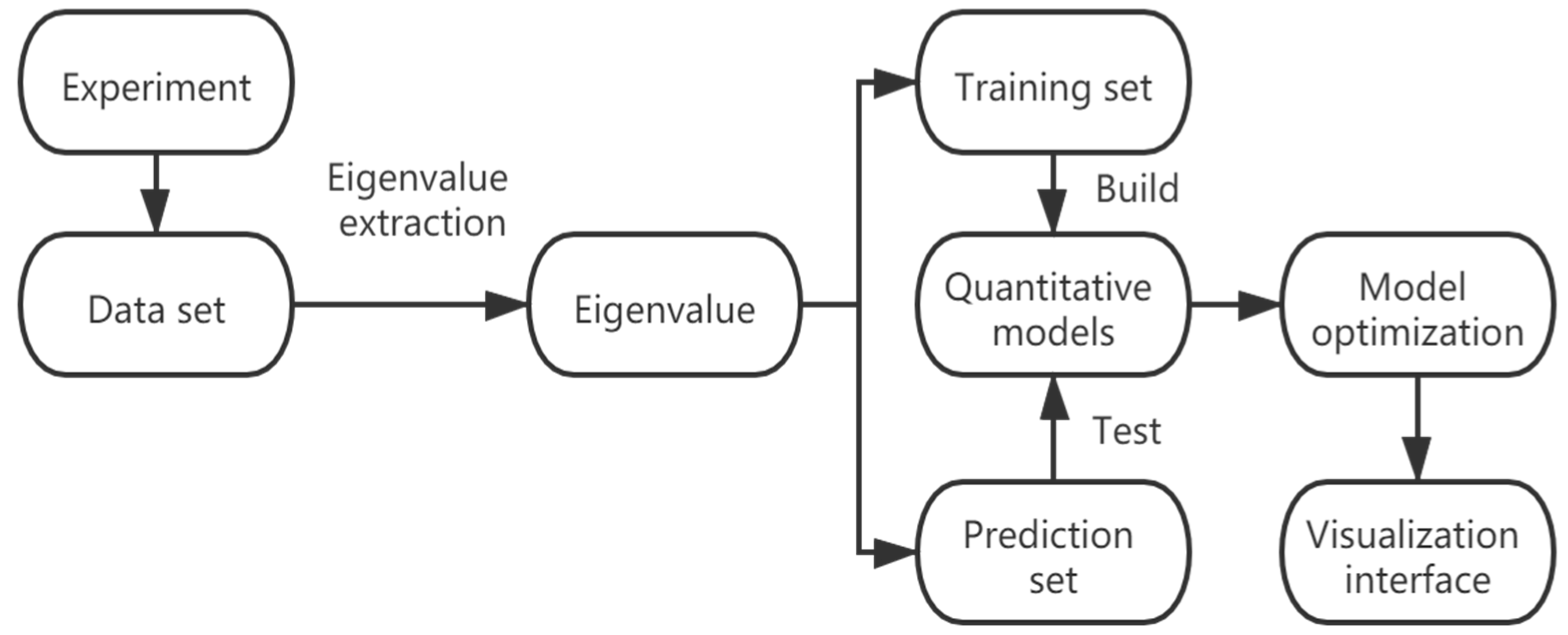
In this section, the analytical procedure of the proposed method was produced briefly. Firstly, the eigenvalue of EEM spectra were extracted using Contour Projection method [20]. Based on the characteristic values of EEM spectra, variables were preliminarily filtered by stepwise regression. Secondly, the dataset was divided into training set and prediction set; then, a multivariate linear regression model for each compound was established using the training set and was validated with the prediction set. Next, the established models were optimized to predict the concentrations of the target compounds in real sample more accurate. Finally, the visualization interface was built up to simplify the operation of the above algorithm. The analytical procedure is shown in Figure 1.
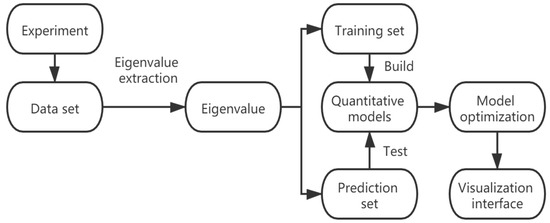
Figure 1.
The flow chart of the analytical procedure.
2.3. Eigenvalue Extraction
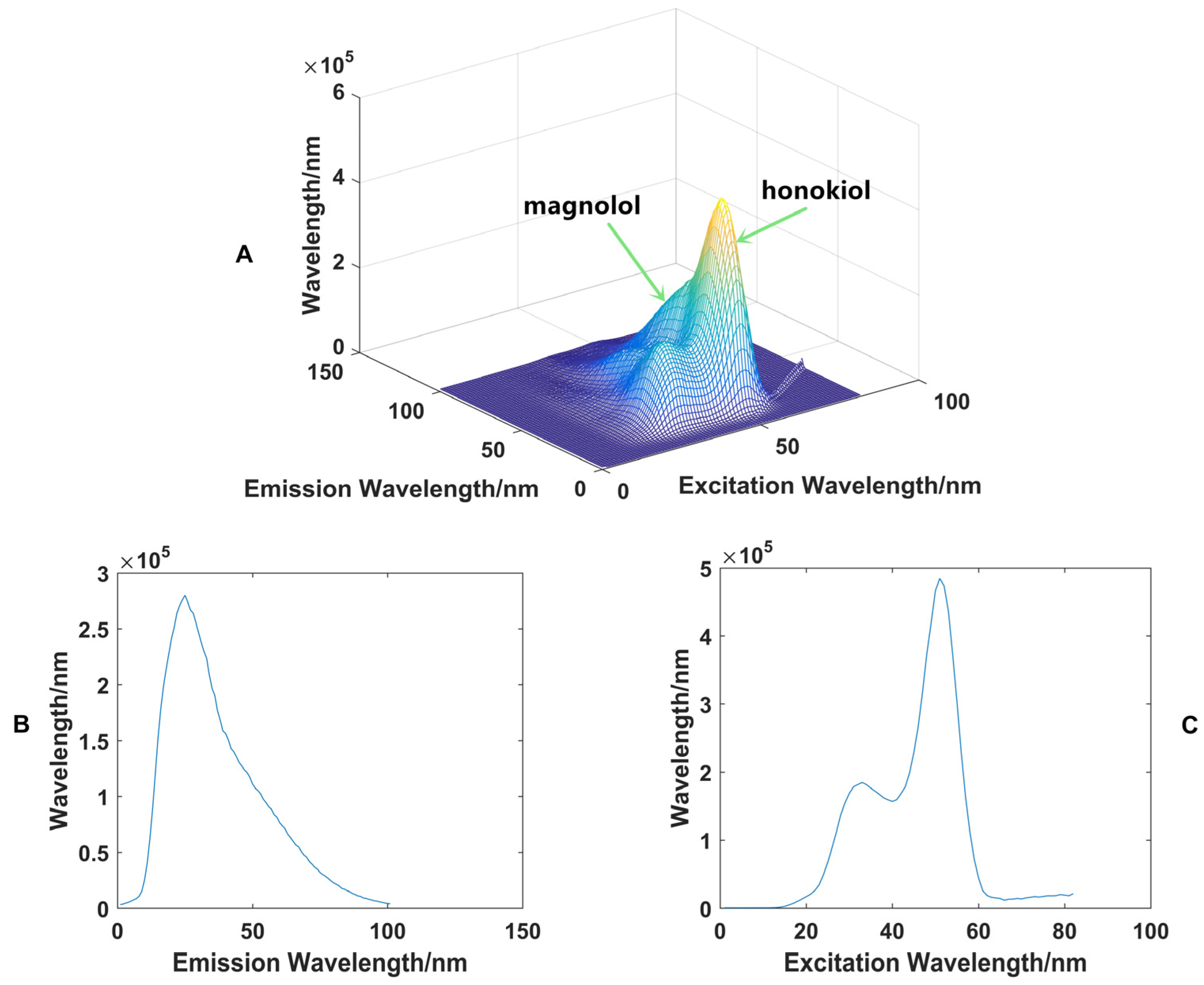
In order to quickly analyze and predict the concentrations of the target component in the sample, the eigenvalues of the EEM spectra (Figure 2A) in different wavelength directions were extracted, that is, the maximum absorption values in different wavelength directions were extracted [21]. Figure 2B shows the maximum absorption intensity extracting from emission wavelength direction. Figure 2C shows the maximum absorption intensity extracting from excitation wavelength direction. As shown in Figure 2C, the extracted eigenvalues in the direction of the excitation wavelength only reflected the signal value of magnolol, so the eigenvalues in the direction of the emission wavelength (Figure 2B) were employed for subsequent quantitative analysis studies, which yielded 101 data points per analyzed sample [22,23,24].
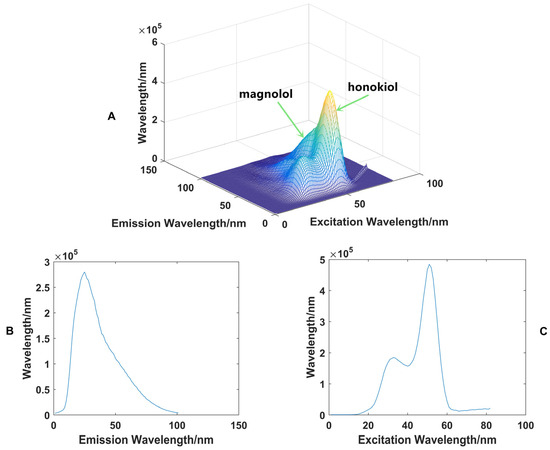
Figure 2.
The EEM spectrum of a sample (A), the eigenvalues extracted from the direction of the emission wavelength (B), and excitation wavelength (C).
To facilitate subsequent processing, the data table was arranged as shown in Table 1, in which 23 rows represented the characteristic values of 23 different sets of samples. In total, 101 columns represented the maximum absorption intensity at different emission wavelength, the header of each column of the table was named with any different letter (for example A, B, C… AA, AB, AC… DA, DB, DC in this work), and the last column named “Pre” represented the concentration of a target compound.

Table 1.
Data arrangement of eigenvalues.
2.4. Principle of the Multiple Linear Regression Model
The multiple linear regression model is based on multiple independent variables x to predict a dependent variable y, Equation (1) is the form of multiple linear regression model [25]. In this paper, the absorption intensity value was substituted into Equation (1) to obtain the corresponding coefficient and constant term, and finally, the multiple linear regression model was obtained.
For the selection of the independent variable x, the stepwise regression method [26] was employed. Here, the selected eigenvalues were defined as x, and the concentration values were denoted as y. After multivariate linear model was established, the model needs to be analyzed for hypothesis testing by the following steps [27]:
- (1)
- The null hypotheses and alternative hypotheses for raising the question.
- (2)
- Conditional on the null hypothesis, the construct statistic F.
- (3)
- According to sample information, calculate the value of statistics.
Comparing the value of sample F with the value of theoretical F distribution, if the sample value F in Equation (3) is less than the theoretical value, the original hypothesis—that there is no regression relationship between variable x and y—can be accepted, and then the hypothesis test ends. If the sample value F is larger than the theoretical value and rejects the original hypothesis, Student’s t-test should further be performed to determine which explanatory variables are important and which are not.
In this paper, the F-test [28] was performed on the above mathematical model, and the sample value F = 53.94 and the theoretical value F = 3.41 were obtained. By comparison, the sample value F was much larger than the theoretical value, rejecting the original hypothesis, and the next test could be carried out.
Next, we conducted Student’s t-test [28] and construct statistics according to Formula (4).
Then, we can judge whether the variable passes the significance test of the coefficient, so as to determine whether the variables in the model are the important factors for predicting the concentration.
2.5. Model Validation
To enhance the understanding of the performance evaluation methods used in the study, it is important to elaborate on how each model’s efficiency was gauged using specific statistical metrics. The performance of each established model was primarily evaluated by two key statistical parameters: the correlation coefficient of prediction (RP) and the root mean square error of prediction (RMSEP) [29]. The calculation of RP is as per Equation (5), and the calculation of RMSEP is as per Equation (6).
These metrics measure the consistency between the model’s predictions and the actual data. The range was from −1 to 1, where 1 indicates perfect prediction, 0 indicates no correlation, and −1 indicates a perfect negative correlation.
This metric measures the average magnitude of the error between the predicted values and the actual values. The goal is to have a low RMSEP, indicating high precision in predictions.
These metrics provide a quantitative assessment of the model’s predictive accuracy and precision.
3. Results and Discussion
3.1. The Establishment of the Model
Before the model establishment, 80% of the samples were randomly selected as the training set for the establishment of the quantitative analysis model, and the remaining 20% as the test set to verify the predictive ability of the established model.
In this paper, stepwise regression method was used for model establishment on the basis of training set. The variables initially selected were in column 6, 42, and 43 of the table, named F, AR and AQ, respectively (as illustrated in Table 1). As introduced in Section 2.4, the test value of the intercept term and the corresponding variables in columns F, AR, and AQ were less than 0.05, which indicates that these variables had all passed the significance test of the coefficient; in the model, these variables were important factors affecting the concentrations.
According to Equation (1), a multiple linear regression model was established, and the multiple linear equation for predicting the concentration of magnolol is shown in Equation (7). Similarly, the multiple linear equation for predicting the concentration of honokiol is shown in Equation (8).
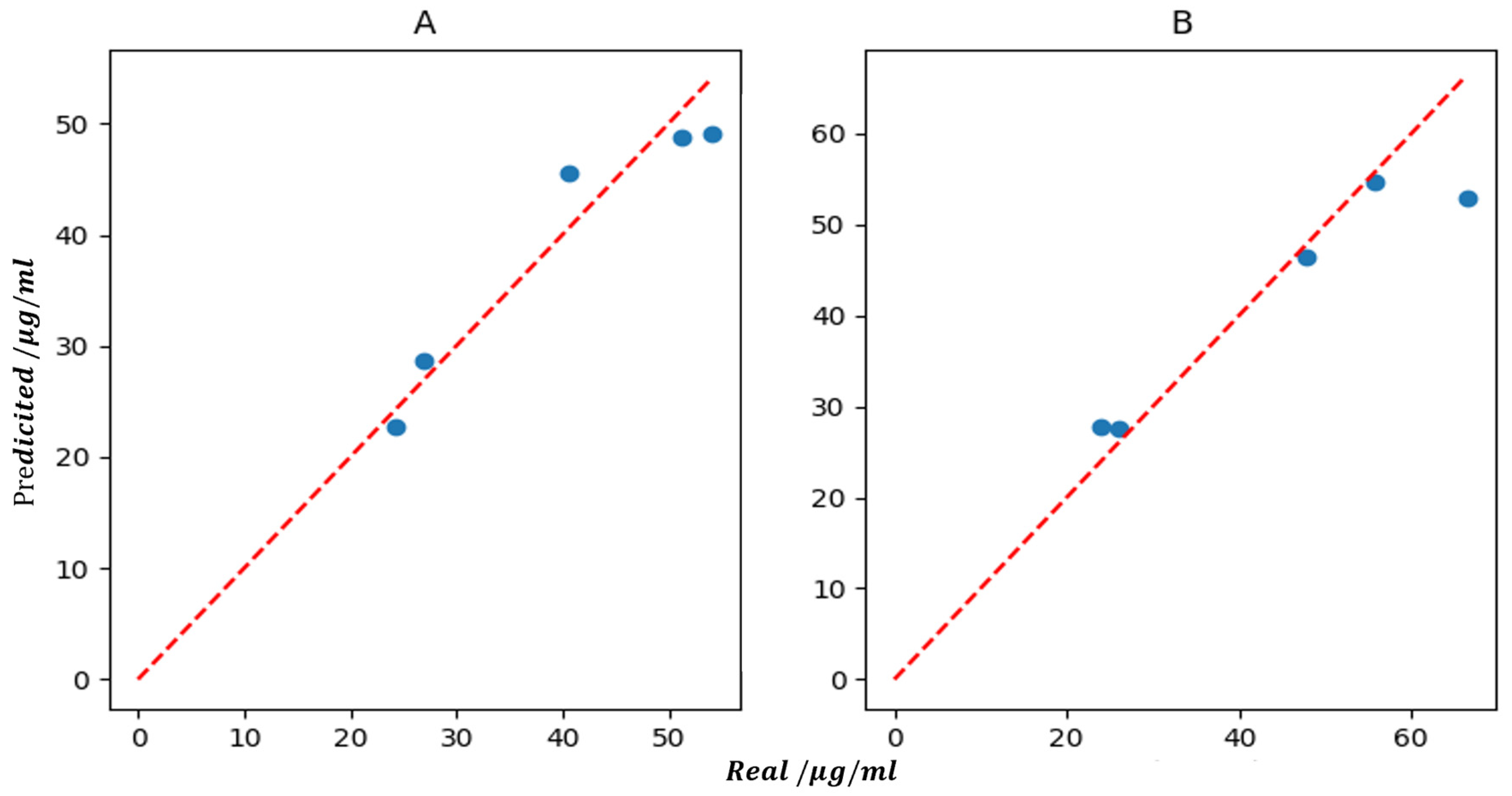
Then, the established models were applied to predict the concentrations of magnolol and honokiol in test set. The predicted and actual values in the test set are shown in Table 2. To easily check the performance of the established models, the relationship between the predicted values and the actual ones of the two target compounds is illustrated in Figure 3. Here, the Rp values for magnolol and honokiol were 0.9599 and 0.9665, respectively, and the RMSEP values were 12.1748 and 36.8144, respectively. According to the above parameter values, the model could be further optimized to improve the accuracy.

Table 2.
The predicted concentrations calculated on the basis of the established models and actual values of the two target compounds in test set.
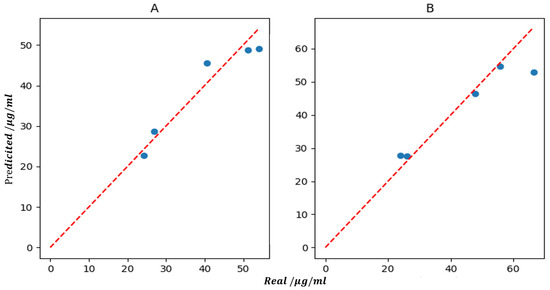
Figure 3.
The relationship between the predicted values and the real ones of magnolol (A) and honokiol (B).
3.2. Model Optimization and Result Analysis
3.2.1. Model Optimization
A normal distribution test can be performed on the model first. The premise of establishing a linear regression model is that the residual items conform to the law of normal distribution.
The dependent variable in the essence equation follows a normal distribution, and the normal distribution expression is shown in Equation (9):
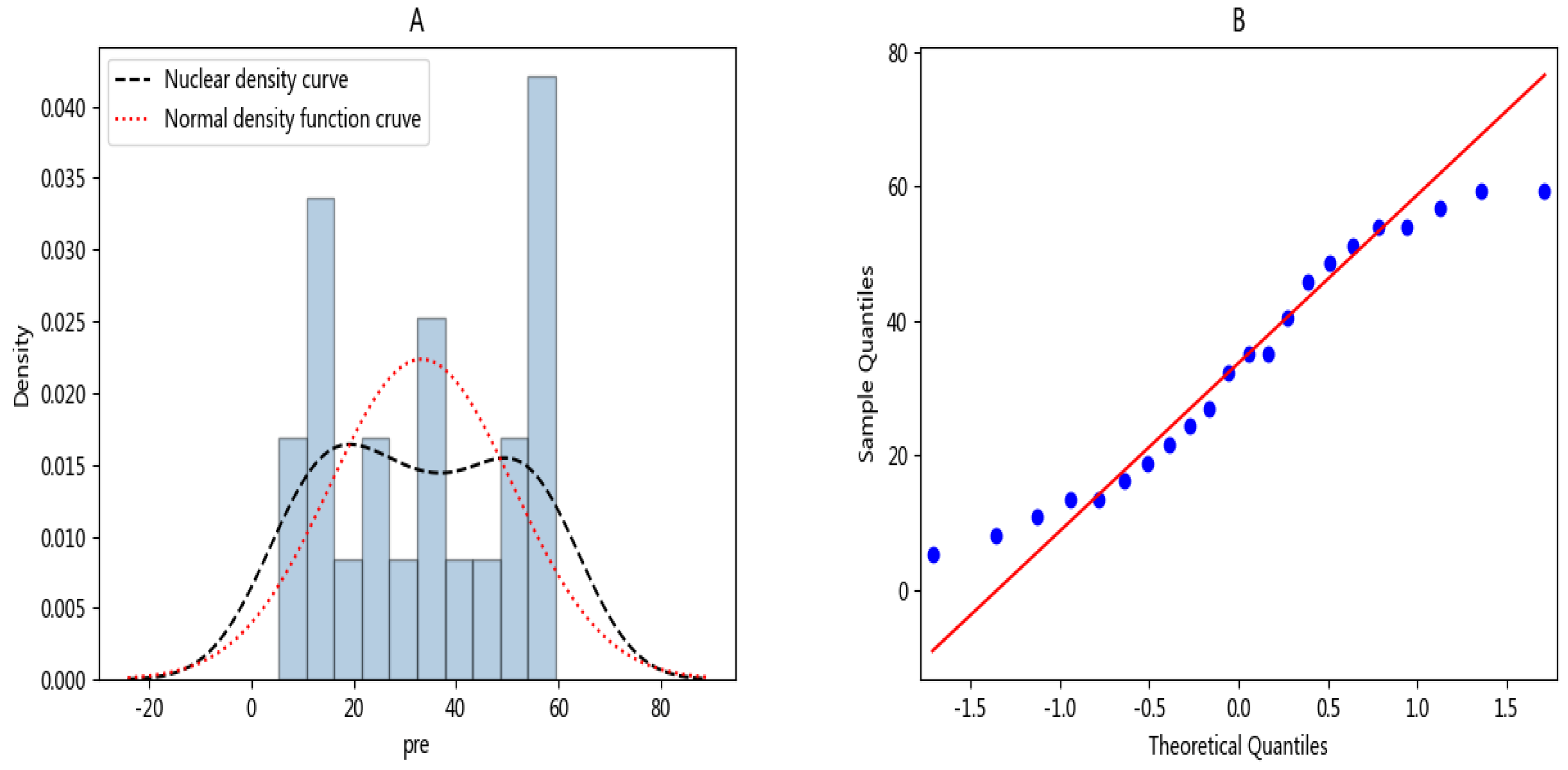
According to the data in the sample, we can make the normal density distribution map (Figure 4). As shown in Figure 4A, we can observe that the data basically conformed to the normal distribution law, so we could further make the Q-Q map of the model and continue to test the normal distribution of the data. Let the x-axis be the quantile of the normal distribution, and the y-axis be the sample quantile. As shown in Figure 4B, the points formed by the two were distributed in a straight line and obeyed the normal distribution.
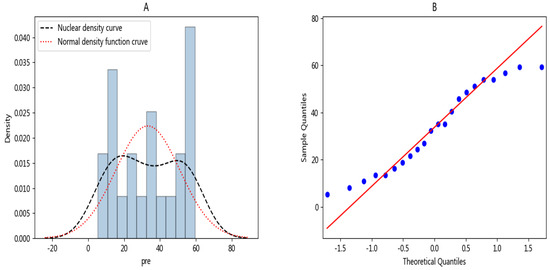
Figure 4.
(A) Normal density distribution diagram, (B) quantile-quantile diagram.
A linear correlation test between the variable x in the model and the concentration value y can be performed to ensure that there is a linear relationship between the independent and dependent variables used for modeling. Regarding the judgment of linear relationships, we could identify them using Pearson’s correlation coefficient [30] and visualization methods. Since the method of visualization gives more intuitive results, in this paper, we chose visualization to examine it and plot all the variables x and concentration y (Figure 5), so that the direct linear correlation between x and y could be found accurately. As illustrated in the red rectangle in Figure 5, a good linear relationship between the independent variables F, AR, and AQ and the concentration was found.
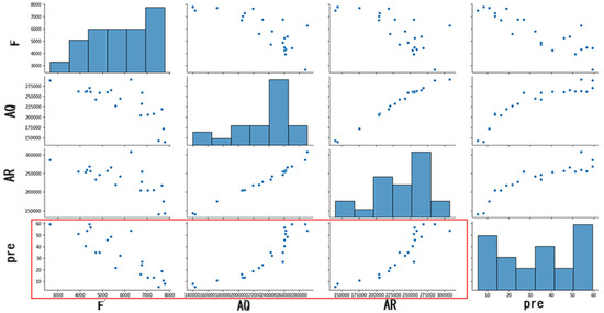
Figure 5.
Linear relationship diagram.
3.2.2. Results Analysis
After the above optimization process, the models can be established again according to the selected variables. According to Figure 5, there was a clear linear relationship between the F column, AR column, AQ column and concentrations of magnolol y. Therefore, the variables F, AR and AQ were selected in the variable set to establish the model again, and the final multiple linear model is shown in Equation (10):
Similarly, the optimized model for honokiol is shown in Equation (11)
The predicted concentrations and actual ones of the two target compounds in the test set derived from the above models are shown in Table 3, and the validation parameters of the model are shown in Table 4. According to the parameters of the test set and the relationship between the predicted values and the actual ones, the accuracy of the optimized model was improved, demonstrating that the optimization process was necessary. The obtained results demonstrated that the proposed strategy can be applied to quantitative determination of the magnolol and honokiol on the basis of EEM spectra even in the presence of overlapping.

Table 3.
The predicted concentrations calculated on the basis of the optimized models and actual values of the two target compounds in the test set.

Table 4.
Parameters of the optimized models.
4. Graphical User Interface
In order to allow users to easily use the above modeling methods without the requirement of programming experiences, a user-friendly graphical user interface (GUI) (Figure 6) that comprised the above process was developed and released freely. The users only need to upload the data table after preliminary processing in this interface and input the header of the defined variable column and concentration column in the input field; then, they can establish a model to predict and analyze the concentration [31]. Here, a step-by-step description of how to use the GUI is given.

Figure 6.
The developed graphical user interface.
The text input box (1) can input the required data table, which must be excel format, and the table format is shown in Table 1.
Button (2) can call the local file list of the computer, and a data table can be selected and uploaded. After selection, the address of the data table will be displayed in the text box (1), or the file address can be directly entered in the text box (1) if the user knows the location of the file in the computer.
Button (3) is the submit button. If no local file is selected, when the user clicks button (3) to submit, a command prompt box will pop up to prompt the user to submit the data table [31]. If the data table has been selected, the prompt box shows that the data table has been uploaded successfully.
The text input box (4) is used to enter the name of the defined variable y (concentration) (in this paper, the header of y is defined as pre, as shown in Table 1).
The button (5) is the submit button. If the user does not input data in the text input box (4), a command prompt window will pop up when clicking the button (5). When the variable name is entered and the button is clicked, the system prompts the data submission to succeed.
The text input box (6) is used to define the name of x, with plus signs separating the different variable names, as defined in this paper. For variables F, AR and AQ, they should be entered as ‘F + AR + AQ’.
The button (7) is the submission button, if the user does not enter the data in the text entry box (6), the system will prompt to enter the data when clicking the button (7). If variable entry is followed by clicking on the button (7), variable entry success is shown.
The button (8) is the submit button. If the user inputs data in the text input boxes (4) and (6), a command prompt that shows successful entry of the variant when clicking on the button (8) If there is no variable input, the command prompt window of please input your data will pop up.
Button (9) is the plot button. Click this button to pop up the diagram of concentration values and the predicted ones, as shown in Figure 2.
The button (10) is the display result button. After clicking, the actual concentrations and the prediction results including predicted concentrations and the model information (intercept, coefficient of each selected variables) can be displayed as illustrated in Figure S1.
The function of the right part of the GUI is the model optimization. The linear relationship between the variable x and the concentration y can be shown as Figure 3 while click button (12).
The text input box (13) inputs the filtered variable x that have linear relationship with y, and the operation is the same as the text input box (6).
The operation mode of the button (14) is the same as that of the button (7).
The function of buttons (15) and (16) are the same as buttons (8) and (9). The optimized results are shown in (17).
5. Conclusions
The contour projection value of the EEM spectra can be regarded as the representative features of the target compounds to some extent; therefore, it can be used to quantitative determination of target compounds. By the application of the extracted contour projection values, the complexity of the processing for EEM analysis was reduced, and the analysis efficiency was improved. In the present study, an efficient strategy that combined with contour projection values, stepwise regression and multiple linear regression modeling methods was developed for quantitative determination of two partially overlapped compounds. By the application of the proposed method, the model can be established, diagnosed and optimized to ensure its reliability and realize the purpose of accurately predict the concentrations of the target compounds in actual sample. Finally, a user-friendly GUI has been released, which makes the proposed strategy easily customizable [27].
Supplementary Materials
The following supporting information can be downloaded at: https://www.mdpi.com/article/10.3390/sym16070922/s1, Figure S1: Data presentation interface; Table S1: Solution concentrations of mixed standard solution.
Author Contributions
Methodology: X.L. and L.T.; formal analysis: Z.C.; investigation: Z.C.; software: X.L.; writing: X.L.; review and editing: J.G. and B.L.; supervision: B.L. All authors have read and agreed to the published version of the manuscript.
Funding
This research was funded by the Project of Young Innovative Talents in Colleges and Universities in Guangdong Province, grant number 2018KQNCX263; Jiangmen Program for Innovative Research Team, grant number 2018630100180019806; Jiangmen City Science and Technology Basic Research Project, grant number 2020030102060005412; and the team project of Wuyi University, grant number 2019td09. The APC was funded by High-level Talents for Scientific Research, grant number 2018AL007.
Data Availability Statement
The data is contained within the GitHub link: https://github.com/xinkangli/graphical-user-interface (accessed on 1 January 2024).
Conflicts of Interest
The authors have declared no conflicts of interest.
References
- Ndou, T.T.; Warner, I.M. Applications of multidimensional absorption and luminescence spectroscopies in analytical chemistry. Chem. Rev. 1991, 91, 493–507. [Google Scholar] [CrossRef]
- Gabor, R.S.; Baker, A.; McKnight, D.M.; Miller, M.P. Fluorescence indices and their interpretation. Aquat. Org. Matter Fluoresc. 2014, 303. [Google Scholar] [CrossRef]
- Kumar, K.; Mishra, A.K. Analysis of dilute aqueous multifluorophoric mixtures using excitation–emission matrix fluorescence (EEMF) and total synchronous fluorescence (TSF) spectroscopy: A comparative evaluation. Talanta 2013, 117, 209–220. [Google Scholar] [CrossRef] [PubMed]
- Andrade-Eiroa, A.; Canle, M.; Cerda, V. Environmental applications of excitation-emission spectrofluorimetry: An in-depth review I. Appl. Spectrosc. Rev. 2013, 48, 1–49. [Google Scholar] [CrossRef]
- Liu, Z.; Zhao, H.; Yang, G.; He, K.; Sun, X.; Wang, Z.; Wang, D.; Qiu, J. Study of photodegradation kinetics of aflatoxins in cereals using trilinear component modeling of excitation-emission matrix fluorescence data. Spectrochim. Acta A Mol. Biomol. Spectrosc. 2020, 235, 118266. [Google Scholar] [CrossRef] [PubMed]
- Peng, N.; Wang, K.F.; Tu, N.Y.; Liu, Y.; Li, Z.L. Fluorescence regional integration combined with parallel factor analysis to quantify fluorescencent spectra for dissolved organic matter released from manure biochars. RSC Adv. 2020, 10, 31502–31510. [Google Scholar] [CrossRef] [PubMed]
- Liu, T.; Li, X.G.; Wang, J.Y.; Liu, D.L.; Wei, Y.J. Time-resolved fluorescence and chemometrics-assisted excitation-emission fluorescence for qualitative and quantitative analysis of scopoletin and scopolin in Erycibe obtusifolia Benth. Spectrochim. Acta A Mol. Biomol. Spectrosc. 2019, 219, 96–103. [Google Scholar] [CrossRef]
- Hemmilá, I.; Mukkala, V.-M. Time-resolution in fluorometry technologies, labels, and applications in bioanalytical assays. Crit. Rev. Clin. Lab. Sci. 2001, 38, 441–519. [Google Scholar] [CrossRef]
- Zhang, T.; Tang, H.; Li, H. Chemometrics in laser-induced breakdown spectroscopy. J. Chemom. 2018, 32, e2983. [Google Scholar] [CrossRef]
- Alcaraz, M.R.; Morzan, E.; Sorbello, C.; Goicoechea, H.C.; Etchenique, R. Multiway analysis through direct excitation-emission matrix imaging. Anal. Chim. Acta 2018, 1032, 32–39. [Google Scholar] [CrossRef] [PubMed]
- Yuan, Y.-Y.; Wang, S.-T.; Wang, J.-Z.; Cheng, Q.; Wu, X.-J.; Kong, D.-M. Rapid detection of the authenticity and adulteration of sesame oil using excitation-emission matrix fluorescence and chemometric methods. Food Control 2020, 112, 107145. [Google Scholar] [CrossRef]
- Yin, X.-L.; Wu, H.-L.; Gu, H.-W.; Hu, Y.; Xia, H.; Wang, L.; Yu, R.-Q. Second-order calibration method applied to process three-way excitation–emission-kinetic fluorescence data: A novel tool for real-time quantitative analysis of the lactone hydrolysis of irinotecan in human plasma. Chemom. Intell. Lab. Syst. 2015, 146, 447–456. [Google Scholar] [CrossRef]
- Vosough, M.; Eshlaghi, S.N.; Zadmard, R. On the performance of multiway methods for simultaneous quantification of two fluoroquinolones in urine samples by fluorescence spectroscopy and second-order calibration strategies. Spectrochim. Acta A Mol. Biomol. Spectrosc. 2015, 136 Pt B, 618–624. [Google Scholar] [CrossRef]
- Perez, A.L.; Tibaldo, G.; Sanchez, G.H.; Siano, G.G.; Marsili, N.R.; Schenone, A.V. A novel fluorimetric method for glyphosate and AMPA determination with NBD-Cl and MCR-ALS. Spectrochim. Acta A Mol. Biomol. Spectrosc. 2019, 214, 119–128. [Google Scholar] [CrossRef] [PubMed]
- Tan, L.; Zhang, Y.; Yang, Q.; Chen, N.; Du, W.; Tang, L.J.; Jiang, J.H.; Yu, R.Q. A novel algorithm for second-order calibration of three-way data in fluorescence assays of multiple breast cancer-related DNAs. Talanta 2019, 195, 433–440. [Google Scholar] [CrossRef] [PubMed]
- Bai, X.M.; Liu, T.; Liu, D.L.; Wei, Y.J. Simultaneous determination of alpha-asarone and beta-asarone in Acorus tatarinowii using excitation-emission matrix fluorescence coupled with chemometrics methods. Spectrochim. Acta Part. A-Mol. Biomol. Spectrosc. 2018, 191, 195–202. [Google Scholar] [CrossRef] [PubMed]
- Zareef, M.; Chen, Q.; Ouyang, Q.; Kutsanedzie, F.Y.H.; Hassan, M.M.; Viswadevarayalu, A.; Wang, A. Prediction of amino acids, caffeine, theaflavins and water extract in black tea using FT-NIR spectroscopy coupled chemometrics algorithms. Anal. Methods 2018, 10, 3023–3031. [Google Scholar] [CrossRef]
- Amneh, A.A.-M. Application of Moving Average Filter for the Quantitative Analysis of the NIR Spectra. J. Anal. Chem. 2019, 74, 686–692. [Google Scholar] [CrossRef]
- Yang, Y.; Zhang, J.; Jin, H.; Zhang, J.; Wang, Y. Quantitative Analysis in Combination with Fingerprint Technology and Chemometric Analysis Applied for Evaluating Six Species of Wild Paris Using UHPLC-UV-MS. J. Anal. Methods Chem. 2016, 2016, 3182796. [Google Scholar] [CrossRef] [PubMed]
- Li, B.Q.; Chen, J.; Li, J.J.; Wang, X.; Zhai, H.L.; Zhang, X.Y. High-performance liquid chromatography with photodiode array detection and chemometrics method for the analysis of multiple components in the traditional Chinese medicine Shuanghuanglian oral liquid. J. Sep. Sci. 2015, 38, 4187–4195. [Google Scholar] [CrossRef] [PubMed]
- Jing, Z.-B.; Wang, W.-L.; Nong, Y.-J.; Zhu, P.; Lu, Y.; Wu, Q.-Y. Fluorescence analysis for water characterization: Measurement processes, influencing factors, and data analysis. Water Reuse 2023, 13, 33–50. [Google Scholar]
- Nie, J.-F.; Wu, H.-L.; Wang, J.-Y.; Liu, Y.-J.; Yu, R.-Q. The chemical rank estimation for excitation-emission matrix fluorescence data by region-based moving window subspace projection technique and Monte Carlo simulation. Chemom. Intell. Lab. Syst. 2010, 104, 271–280. [Google Scholar] [CrossRef]
- Wu, H.-L.; Wang, T.; Yu, R.-Q. Recent advances in chemical multi-way calibration with second-order or higher-order advantages: Multilinear models, algorithms, related issues and applications. Trends Anal. Chem. 2020, 130, 115954. [Google Scholar] [CrossRef]
- Hu, L.; Yin, C. Multi-way calibration coupling with fluorescence spectroscopy to determine magnolol and honokiol in herb and plasma samples. Anal. Methods 2015, 7, 5913–5923. [Google Scholar] [CrossRef]
- Jones, D.M.; Watton, J.; Brown, K.J. Comparison of hot rolled steel mechanical property prediction models using linear multiple regression, non-linear multiple regression and non-linear artificial neural networks. Ironmak. Steelmak. 2013, 32, 435–442. [Google Scholar] [CrossRef]
- Yuan, L.; Li, L.; Zhang, T.; Chen, L.; Liu, W.; Hu, S.; Yang, L. Modeling Soil Moisture from Multisource Data by Stepwise Multilinear Regression: An Application to the Chinese Loess Plateau. ISPRS Int. J. Geo-Inf. 2021, 10, 233. [Google Scholar] [CrossRef]
- Kim, K.H.; Chao, S.K.; Hardle, W.K. Simultaneous inference of the partially linear model with a multivariate unknown function. J. Stat. Plan. Inference 2021, 213, 93–105. [Google Scholar] [CrossRef]
- Luepsen, H. ANOVA with binary variables: The F-test and some alternatives. Commun. Stat.-Simul. Comput. 2023, 52, 745–769. [Google Scholar] [CrossRef]
- Zhang, W.; Li, N.; Feng, Y.; Su, S.; Li, T.; Liang, B. A unique quantitative method of acid value of edible oils and studying the impact of heating on edible oils by UV-Vis spectrometry. Food Chem. 2015, 185, 326–332. [Google Scholar] [CrossRef] [PubMed]
- Alsaqr, A.M. Remarks on the use of Pearson’s and Spearman’s correlation coefficients in assessing relationships in ophthalmic data. Afr. Vis. Eye Health 2021, 80, 10. [Google Scholar] [CrossRef]
- Mishra, P. CT-GUI: A graphical user interface to perform calibration transfer for multivariate calibrations. Chemom. Intell. Lab. Syst. 2021, 214, 104338. [Google Scholar] [CrossRef]
Disclaimer/Publisher’s Note: The statements, opinions and data contained in all publications are solely those of the individual author(s) and contributor(s) and not of MDPI and/or the editor(s). MDPI and/or the editor(s) disclaim responsibility for any injury to people or property resulting from any ideas, methods, instructions or products referred to in the content. |
© 2024 by the authors. Licensee MDPI, Basel, Switzerland. This article is an open access article distributed under the terms and conditions of the Creative Commons Attribution (CC BY) license (https://creativecommons.org/licenses/by/4.0/).

