Flow Effects and Propulsion Performance on Various Single Expansion Ramp Nozzle Configurations of Scramjet Engine

Abstract

This study serves as a research endeavor aiming to explore the behavior of the coupling flow effects of the single expansion ramp nozzle (SERN) in over-expansion conditions during the static start-up process. The open-source program OpenFOAM and its solver “rhoCentralFoam” are employed in the 2D simulation and the two critical geometric variations, the shape of the ramp and the length of the flap beyond the throat, are considered in the geometric variation. The result shows the preferable propulsion performance in the FSS (Free Shockwave Separation) state compared to RSS (Restricted Shockwave Separation). FSS also plays the role of the initial, albeit transient, separation, which originates from the shockwave from the throat and will eventually transform into a stabler RSS state. For the 100% flap length configuration in this study, the axial thrust can achieve a high value of 500 N/m in the FSS state and decrease to around 450 N/m, on average, in the RSS state. The trust angle also shows a preferable performance of around −13° in FSS compared to −30° in RSS. Regarding geometric modifications, both modifications, shorting the flap and bell-shaped ramp adjustments, manifest similar effects. Both conical and bell-shaped short flap configurations demonstrate an axial thrust from around 1750 to 1900 N/m and a thrust angle of around −45°. However, the flap shortening, which may demonstrate an attitude compensation effect, exhibits a more pronounced effect compared to the bell-shaped modification.

1. Introduction

Most current hypersonic vehicles are rocket-based, and can easily achieve speeds of more than five Mach in rarefied air at high altitudes. However, they have several disadvantages compared to others, including a relatively high payload, low specific impulse, the need for self-carrying oxidant, and a limited lateral force capacity. Consequently, rocket-based vehicles are typically designed with multiple stages and a vertical takeoff, leading to high operational and fuel costs. Reducing the cost of supersonic and even hypersonic flight is crucial, which has promoted researchers to shift their focus to air-breathing engines. Air-breathing engines offer specific impulses two or three times greater than rocket-based engines in hypersonic flight, and more than ten times greater in low Mach flight. Air-breathing engines are also reusable and utilize the oxidant from the surrounding atmosphere, lowering operating costs and fuel costs while providing a high efficiency, making air-breathing engines highly promising for both military and civic usage [1].

The scramjet engine (supersonic combustion ramjet engine) is considered to be the most promising air-breathing thruster. Unlike traditional thrusters that use rotors to compress the inflow, the scramjet engine relies on the ramjet effect at high Mach numbers, thus making it a simpler structure. This characteristic proves advantageous during the simulation and development process. Moreover, the ramjet effect allows the inflow to be maintained supersonically without the need for subsonic speed reduction, enabling supersonic combustion within the combustion chamber. This eliminates the energy loss associated with traditional compression processes. Despite these advantages, the development and application of scramjet engines are considered to be more challenging than those of rockets. Challenges include the Mach number limitation of the ramjet effect, the flow deflection occurring in the combustion chamber under complex shockwave interactions, the ongoing research into supersonic combustion fuel mixing and flame stabilization mechanisms, and the possible power loss due to the unstart effect. Consequently, fundamental research is necessary to advance the application of scramjets [2,3].

The single expansion ramp nozzle (SERN) presents a potential solution for the scramjet engine. SERNs are usually designed from traditionally symmetric conical or Rao’s bell-shaped nozzles by cutting half or truncated manners [4,5], sometimes combined with inverse design methods [6,7]. Unlike traditional symmetrical nozzles, SERNs have distinct and non-axial symmetric structures. They expend the jet solely on a ramp, leading to asymmetric flow phenomena. This asymmetry offers several advantages, such as a simpler geometry, higher assembly, and the ability to control the jet vector by adjusting the throat. However, it also results in asymmetric shockwaves within the nozzle. These shockwaves introduce additional vertical force and lateral force, leading to unfavorable pitch and yaw moments. The geometry parameters, including the profile of the ramp, the flap length, the angle of the ramp, and the shape of the flap, have a decisive impact on the flow separation pattern and the propulsion performance of SERNs. For example, the internal nozzle expansion ramp and expansion have the most significant influence on the lift and moment, and the length of the SERN is related to drag [8].

Scramjets are designed to operate under specific conditions. However, off-design situations still can occur during certain situations, especially in the nozzle inlet, such as unstart phenomena upstream. Moreover, the start-up and shutdown processes in the nozzle inlet should be considered. Clarifying the separation pattern and potential force changes in such situations is crucial. The most common off-design situation for nozzles is over-expansion in the start-up process. This over-expansion occurs when the pressure of the exhaust gas is decreased more than the external pressure in the nozzle, and when pressure differences or sudden changes in geometry occur, shockwaves are generated, leading to Shock Wave–Boundary Layer Interaction (SWBLI) and causing detachment or reattachment on the walls [5,9]. In over-expansion situations, reattachments can result in different separation patterns [10,11].

Therefore, the objective of this study is to explore the separation patterns and investigate the propulsion performances in over-expansion conditions with different SERN configurations during start-up. The research employs a simplified 2D SERN model simulated using the “rhoCentralFoam” solver in OpenFOAM [12]. “rhoCentralFoam” solver utilizes the Kurganov, Noelle, and Petrova method (KNP method) [13], enabling the calculation of flow fields with complex shockwaves without the need for a Riemann solver or characteristic decomposition [14]. In the simulation, the SERN is designed with an NPR = 20, but the actual simulation is conducted with an NPR = 3 to simulate the over-expansion situation. The simulation is primarily conducted two-dimensionally and the auto mesh generation application is employed. As for geometric variations, two fundamental geometric parameters are considered: the flap length and the contour of the ramp. The initial configuration establishes the flap length as the baseline, which is then systematically shortened to 37.5%, 25%, and 12.5% for detailed examinations. Furthermore, the ramp’s contour has options to adopt either the original conical-shaped (straight-line) design or a modified bell-shaped curve.

2. Methods

2.1. Conservation Equations

2.1.1. Flow Dynamic Model

To accurately capture the complex shockwave interaction, “rhoCentalFoam” is employed, which is based on the assumption of a single ideal fluid and utilizes a Eulerian frame of reference. Equations (1)–(3) govern the flow behavior and are as follows:

Conservation of mass:

$${\displaystyle \frac{\partial \rho }{\partial t}}+\mathsf{\nabla }\cdot \left[\rho \mathit{u}\right]=0$$

(1)

Conservation of momentum:

$${\displaystyle \frac{\partial \left(\rho \mathit{u}\right)}{\partial t}}+\mathsf{\nabla }\cdot \left[\mathit{u}\left(\rho \mathit{u}\right)\right]+\mathsf{\nabla }\cdot p+\mathsf{\nabla }\cdot \mathit{T}=0$$

(2)

Conservation of total energy:

$${\displaystyle \frac{\partial \left(\rho E\right)}{\partial t}}+\mathsf{\nabla }\cdot \left[\mathit{u}\left(\rho E\right)\right]+\mathsf{\nabla }\cdot \left[\mathit{u}p\right]+\mathsf{\nabla }\cdot (\mathit{T}\cdot \mathit{u})+\mathsf{\nabla }\cdot \mathit{j}=0$$

(3)

In these equations, $\rho$ denotes the mass density, $\mathit{u}$ represents the velocity vector, and $p$ corresponds to the pressure. The symbol $\mathit{j}$ represents the heat diffusion flux. $E$ refers to the specific internal energy and $\mathsf{\rho }E$ is the total energy, where $\mathsf{\rho }E={\displaystyle \frac{p}{\mathsf{\gamma }-1}}+{\displaystyle \frac{1}{2}}\mathsf{\rho }$ and $E=e+\left|\mathit{u}\right|/2$. The symbol $\mathit{T}$ is the viscous tensor, where $\mathit{T}=\mathsf{\nu }+{\mathsf{\nu }}_t$. $\mathsf{\nu }$ represents a constant kinematic viscosity, which remains unchanged over time. On the other hand, ${\mathsf{\nu }}_t$ refers to the time-dependent viscous tensor (or turbulent viscous tensor), which is calculated using turbulent models such as RAS (Reynolds Averages Simulation) or LES (Large Eddy Simulation).

In this study, assumptions of a single ideal gas are made. The state equation can be described by $p=\mathsf{\rho }RT$, where $T$ means temperature and can be obtained using the equation $e=C_{v}T={\left(\mathsf{\gamma }-1\right)}^{-1}RT$, $R$ represents an individual gas constant, $Cp$ denotes the constant-pressure specific heat, $Cv$ corresponds to the constant-volume specific heat, and $\mathsf{\gamma }$ means the specific heat capacity, which can be obtained by $\mathsf{\gamma }=Cp/Cv$.

2.1.2. Turbulent Model

To accurately capture the viscous effects and address flow detachments and strong reverse pressure gradient in over-expansion conditions, the k-omega Shear Stress Transport (SST) model of RAS is employed in this study [15]. The SST model is a two-equation model that combines the advantages of the k-omega model and the k-epsilon model. The k-omega model provides a more accurate result near the walls, but it tends to be less accurate in the freestream flow. On the other hand, the k-epsilon model performs well in the freestream flow, but is less accurate near walls. By blending these two models, the SST model achieves a higher accuracy both near walls and in the freestream flow. In OpenFOAM, the SST model used is a modified version [16] released by the author Menter in 2003.

2.2. Computational Methods

2.2.1. Time Discretization

In OpenFOAM, the implementation of basic discretization methods and turbulent models takes advantage of the object orientation of C++. OpenFOAM allows users to employ various discretization methods in its database. For achieving a more precise result, the second-order Crank–Nicolson method is utilized for time discretization, and the equation is as follows:

$${\displaystyle \frac{\partial \mathit{\Psi }}{\partial t}}\approx {\displaystyle \frac{\mathsf{\Delta }\mathit{\Psi }}{\mathsf{\Delta }t}}={\displaystyle \frac{{\mathit{\Psi }}^t-{\mathit{\Psi }}^{t-2}}{2\mathsf{\Delta }t}}$$

(4)

In the equation, $\mathit{\Psi }$ represents the generic tensors. $t$ is used to denote the time, and when it appears as the upper index $t$, such as ${\mathit{\Psi }}^t$, it refers to a certain time step. The upper index $t$ corresponds to the present time step, and when it appears as the upper index, such as$t-1$, it can denote a previous time step.

2.2.2. Space Discretization

“rhoCentralFoam” can utilize either the KT method (Kurganov and Tadmor method) or the KNP method for space discretization. The KNP method is selected in this study because it shows a better capability to capture shockwave positions. The KNP method acts as a type of central upwind method, determining the fluid properties on the surfaces based on one-sided local speeds of propagation and interpolating the fluid properties on the cell’s surfaces by both flow and wave transmissions in a compressible flow field. The discretization of convention, gradient, and Laplacian terms can be denoted as follows:

Convention term:

$$\sum _f{\varphi }_f{\mathit{\Psi }}_f=\sum _f\left[\alpha {\varphi }_{f+}{\mathit{\Psi }}_{f+}+\left(1-\alpha \right){\varphi }_{f-}{\mathit{\Psi }}_{f-}+{\omega }_f\left({\mathit{\Psi }}_{f-}-{\mathit{\Psi }}_{f+}\right)\right]$$

(5)

Gradient term:

$${\int }_V\mathsf{\nabla }\mathit{\Psi }dV={\int }_{S}d\mathit{S}\mathit{\Psi }\approx \sum _f{\mathit{S}}_f{\mathit{\Psi }}_f=\sum _f\left[\alpha {\mathit{S}}_f{\mathit{\Psi }}_{f+}+\left(1-\alpha \right)S_f{\mathit{\Psi }}_{f-}\right]$$

(6)

Laplacian term:

$${\int }_V\mathsf{\nabla }\cdot \left(\Gamma \mathsf{\nabla }\mathit{\Psi }\right)dV={\int }_{S}d\mathit{S}\cdot \left(\Gamma \mathsf{\nabla }\mathit{\Psi }\right)\approx \sum _f{\Gamma }_f{\mathit{S}}_f\cdot {\left(\mathsf{\nabla }\mathit{\Psi }\right)}_f$$

(7)

In the equations, $\mathit{S}$ represents the surface, $V$ corresponds to the volume, and $\Gamma$ means the diffusion coefficient. The subscript $f$ denotes the control surfaces. The subindexes $+$ and $-$ represent the flow directions of inward or outward. Thus, $f_{+}$ and $f_{-}$ represent the flow directions of inward and outward from the cell on its surfaces, respectively. $\varphi$ represents the volumetric flux, and the volumetric flux of a control surface $f$ can be described as the inner product of the control surface ${\mathit{S}}_f$ and the velocity $u_f$. This relationship can be described as ${\varphi }_f={\mathit{S}}_f·u_f$, which only considers the flow speed. The symbol $\alpha$ denotes the weighting factor and ${\omega }_f$ represents the diffusive volumetric flux. Both of them consider both speed and wave transmission. Their equations can be described as follows:

$$\alpha ={\displaystyle \frac{{\psi }_{f+}}{{\psi }_{f+}+{\psi }_{f-}}}$$

(8)

$${\omega }_f=\alpha \left(1-\alpha \right)\left({\psi }_{f+}+{\psi }_{f-}\right)$$

(9)

where the symbol $\psi$ represents the volumetric fluxes associated with the local speed of propagation, ${\psi }_{f+}$ and ${\psi }_{f-}$. The $\psi$ inward and outward from the cells can be calculated as followed:

$${\psi }_{f+}=max\left(c_{f+}\left|{\mathit{S}}_f\right|+{\varphi }_{f+},c_{f-}\left|{\mathit{S}}_f\right|+{\varphi }_{f-},0\right)$$

(10)

$${\psi }_{f-}=max\left(c_{f+}\left|{\mathit{S}}_f\right|-{\varphi }_{f+},c_{f-}\left|{\mathit{S}}_f\right|-{\varphi }_{f-},0\right)$$

(11)

In these equations, $c_{+}$ and $c_{-}$ represent the sound speeds of each direction, and ${\mathrm{c}}_{\pm }=\sqrt{\mathsf{\gamma }\mathrm{R}{\mathrm{T}}_{\pm }}$. $\left|S_f\right|$ corresponds to the area of the control surface.

The methods which involve $f_{+}$ and $f_{-}$ necessitate value interpolation (reconstruction) on each face. This interpolation is performed by blending standard first-order upwind and second-order linear interpolations:

$${\mathit{\Psi }}_{f+}=\left(1-g_{f+}\right){\mathit{\Psi }}_P+g_{f+}{\mathit{\Psi }}_N$$

(12)

where the subindices $P$ and $N$ denote the owner cell, a discussed cell, and the neighboring cell, a cell next to the owner cell, respectively. They are separated by the discussed control surfaces $f$ and play a crucial role in determining the values on the surfaces. $g_{f+}$ represents a weight coefficient determined by $g_{f+}=\beta \left(1-{\omega }_f\right)$, and the symbol $\mathsf{\beta }$ in the equation denotes the limiter function. For this research, the Vanleer limiter is selected due to its convergence ability, as shown in Equation (13):

$$\mathsf{\beta }\left(r\right)={\displaystyle \frac{r+\left|r\right|}{1+r}}$$

(13)

2.3. Mesh Design, Computational Conditions, and Boundary Conditions

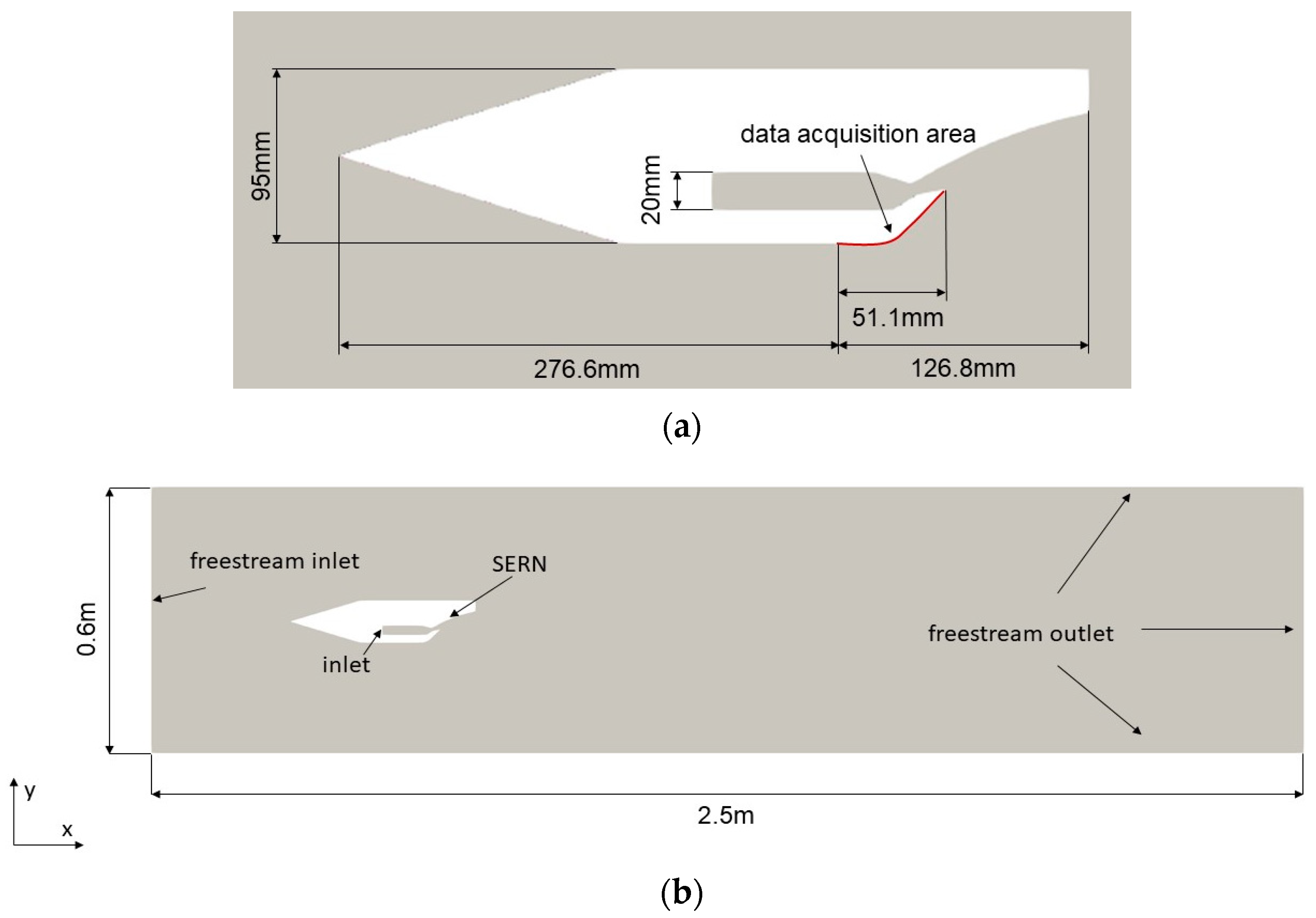
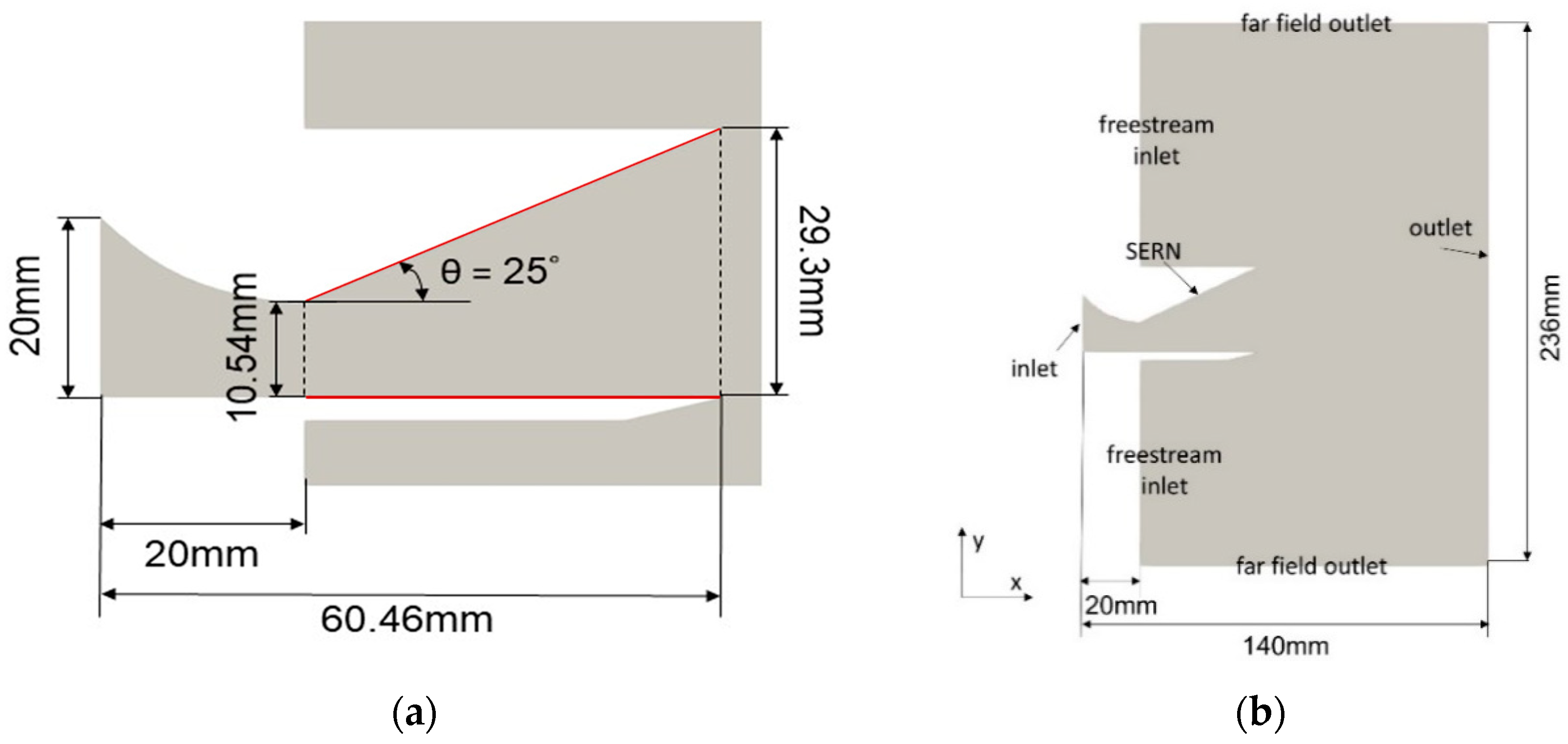
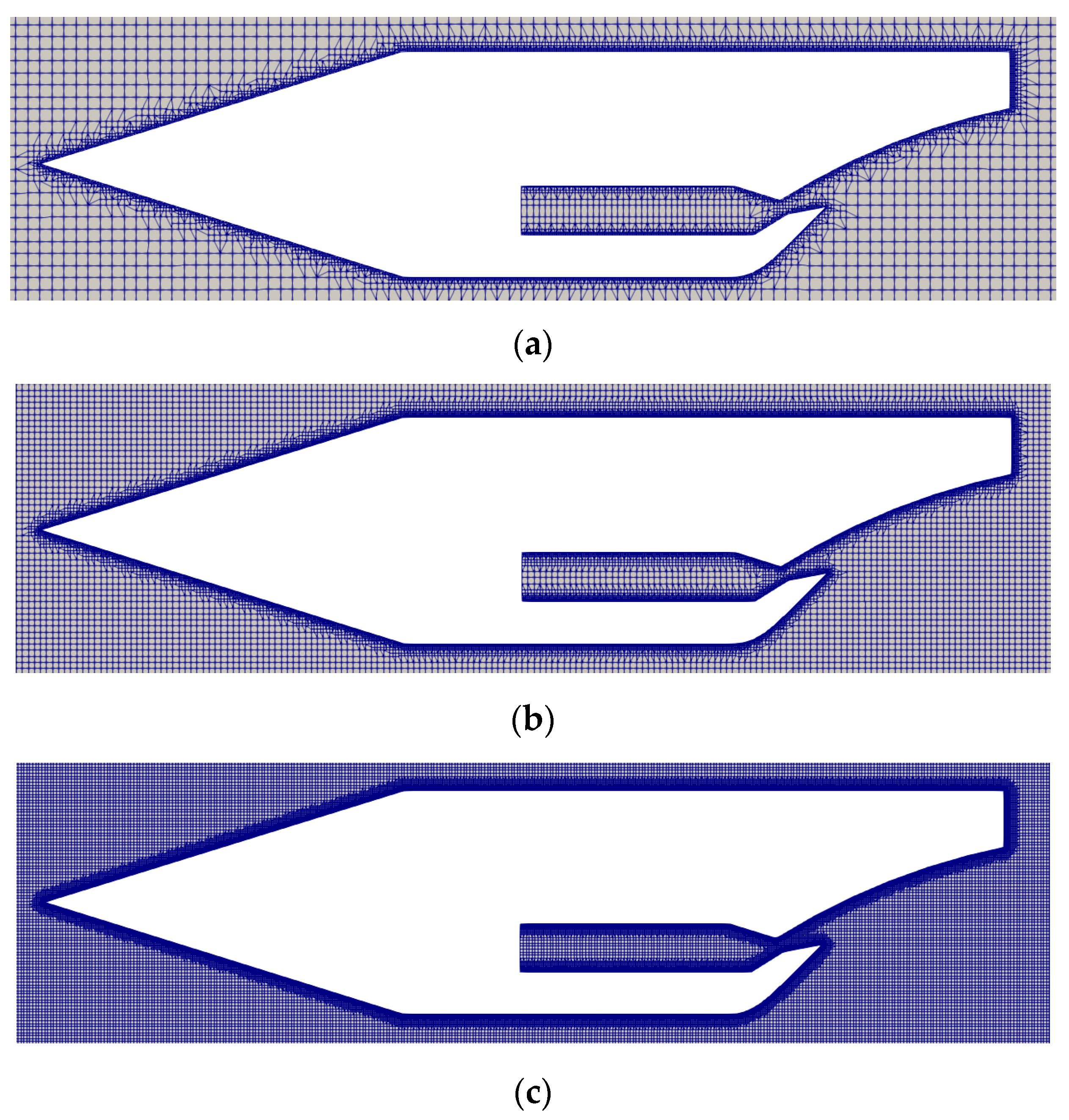
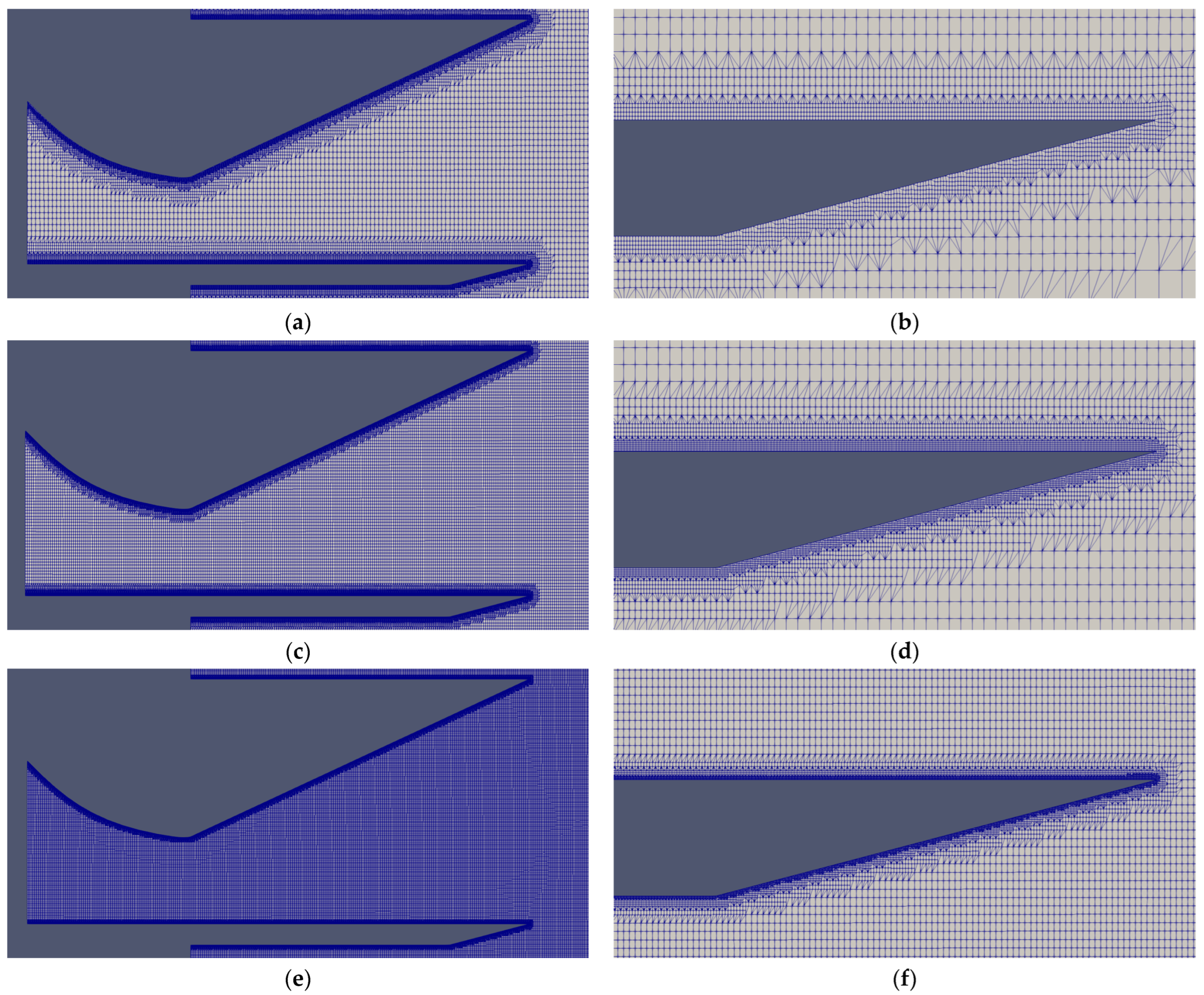
2.3.1. Configuration Design and Mesh Construction Approach

This research is primarily grounded in two distinct geometries: experimental models developed by Gruhn [17] and Yu et al. [5], respectively. To ensure clarity, Gruhn’s model will be referred to as “mesh verification configuration 1”, while Yu et al.’s model will be referred to as “mesh verification configuration 2”.

This research adopts an automatic method utilizing the built-in application “snappyHexMesh” in OpenFOAM [12]. This application generates a mesh using body fitting methods by providing a background mesh and a 3D model as inputs. The “blockMesh” command is used to generate the background mesh, and the commercial package SOLIDWORKS is selected as the software for constructing the 3D model.

2.3.2. Flow Domain and Mesh

Verification Configurations

The research initially establishes the test cases as the mesh verification tests. Mesh verification configuration 1 is developed by DLR (Deutschland für Luft- und Raumfahrt; German Aerospace Center), which includes a wadge in the front and a SERN in the back [17]. The geometry of mesh verification configuration 1 with the surface pressure acquisition area for verification is shown in Figure 1a, and the flow domain (computational domain) pattern is depicted in Figure 1b:

Mesh verification configuration 2 refers to an experiment that places a SERN in the wind tunnel, which is simplified into a SERN jet toward the outer flow domain. Figure 2a shows the SERN’s geometry with the surface pressure acquisition area for verification. Figure 2b denotes the flow domain (computational domain) pattern:

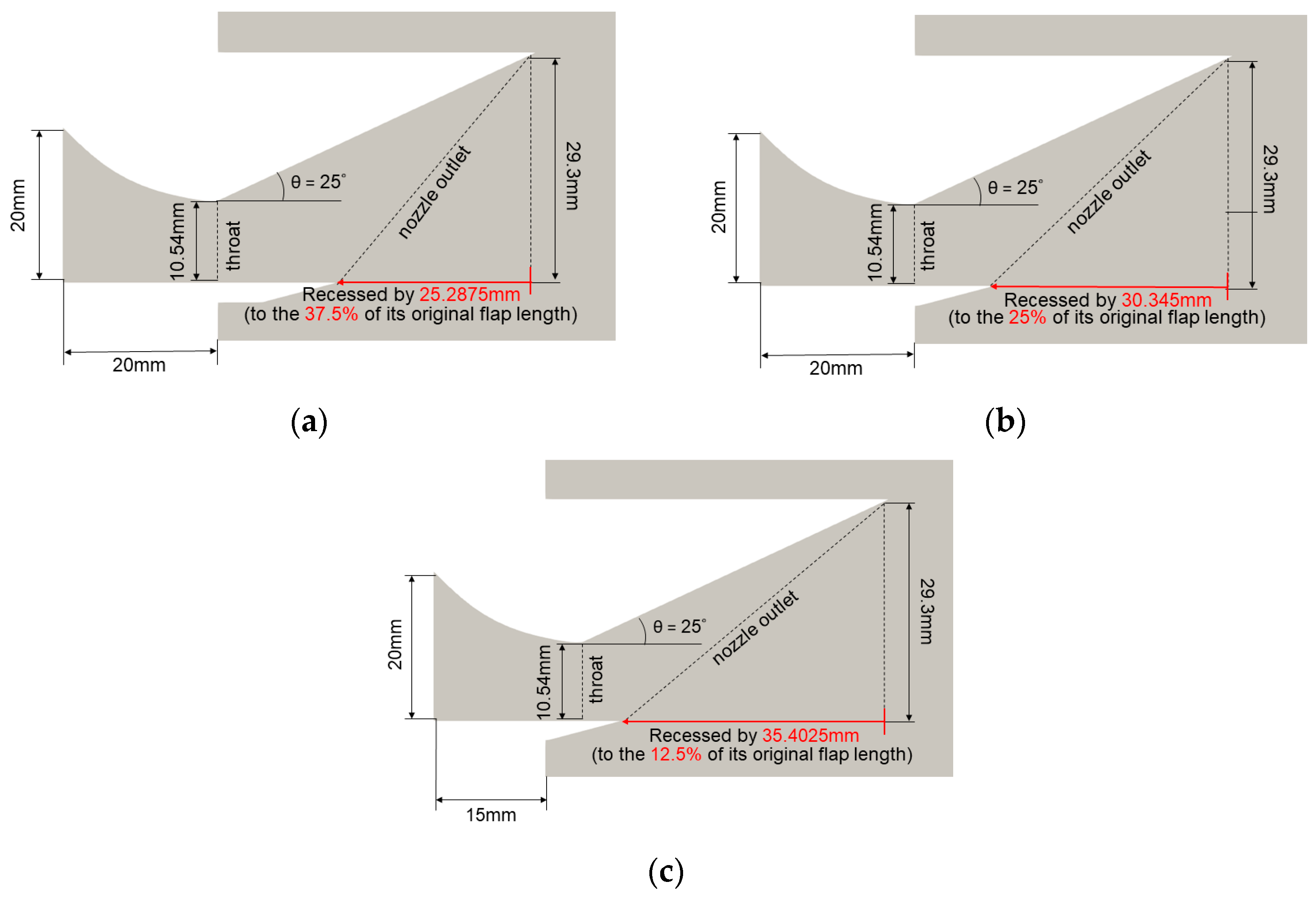
Studied Configurations

The research builds upon the test results of Section 3.1 to develop research configurations. Among the configurations, mesh verification configuration 2 is selected as the fundamental setup, serving as the basis for further modifications to its geometric parameters. The two key parameters under consideration are the shape of the ramp and the length of the flap beyond the throat. In mesh verification configuration 2, the ramp has a conical profile (straight line) in terms of shape, and the flap has the same horizontal length as the ramp, forming a vertical opening. For a clear comparison with the research model in Section 3.2, mesh verification configuration 2 will be described as a conical 100% flap length configuration.

Regarding geometric modification, taking inspiration from the design concept of the aerospike engine [18], the length of the flap is attempted to be reduced to 37.5%, 25%, and 12.5% of the original configuration systematically. To ensure better manageability, these modified configurations will be referred to by the percentage of the original flap length. For example, the configuration with a 37.5% flap length refers to a configuration with a flap length 37.5% of the original flap length, which is equivalent to 15.175 mm. The research configurations mentioned in Section 3.2.1 are illustrated in Figure 3a–c.

In Section 3.2.2, the research configuration undergoes further adjustments, focusing on another crucial parameter: the contour of the ramp. This modification utilizes Rao’s bell-shaped ramp design method [19]. Specifically, the research designs the SERN as a bell-shaped nozzle with a proportion of 60%. The bell-shaped SERN research configurations with 100%, 37.5%, 25%, and 12.5% flap lengths are illustrated in Figure 4a–d.

2.3.3. Boundary Conditions

The simulation adopts boundary conditions based on the corresponding experimental setup. The nozzle entrance utilizes the traditional pressure inlet condition, while the freestream flow inlet usually employs the traditional velocity inlet condition. As for the outlets, either the zero gradient condition or wave transmissive condition are employed. The zero gradient condition assumes that a physical quantity maintains the same value when the flow arrives at the boundaries, hence, the gradient of that quantity is equivalent to zero on the boundary. This boundary condition yields more precise results with a longer computational domain. However, it is possible to reflect the shockwave numerically, leading to divergence in the calculation. Conversely, the wave transmissive condition is used when the possibility of the wave reflection is high, which calculates the values near the computational boundary using characteristic decomposition, enabling shockwaves to transmit across the boundary and obtaining superior results within a relatively narrower computational domain. Regarding the boundary conditions on the walls, the no-slip condition with the wall function is applied. The detailed settings of the velocity, temperature, and pressure for verification configuration 1 are shown in

Table 1. The detailed boundary condition setting of mesh verification configuration 1.

Boundary Conditions	Velocity (m/s)	Pressure (Pa)	Temperature (K)
Freestream inlet	$V_x=673.66,$ $V_y=49.967,V_z$ = 0	7100	55.7
Freestream outlet	“waveTransmissive”	7100	55.7
Nozzle inlet	“zeroGradient”	350,500	269.3
Wall	$V_x=V_y=V_z=0$	“zeroGradient”	“zeroGradient”

.

The boundary conditions used in mesh verification configuration 2 are listed in

Table 2. The detailed boundary condition setting of mesh verification configuration 2 and the research configurations.

Boundary Name	Velocity (m/s)	Pressure (Pa)	Temperature (K)
Nozzle inlet	“zeroGradient”	“zeroGradient”	“zeroGradient”
Freestream outlet	“waveTransmissive”	“waveTransmissive”	“waveTransmissive”
Freestream inlet	“slip”	“zeroGradient”	“zeroGradient”

. It is noteworthy that the freestream inlet of mesh verification configuration 2 in the corresponding simulation exhibits characteristics similar to a wall condition, which can be speculated that the boundary is closed when dealing with verification. Consequently, the ideal slip wall condition, rather than a velocity inlet condition, is applied to the freestream inlet of mesh verification configuration 2.

2.3.4. Mesh Verification Conditions for Configuration 1

As mentioned before, mesh verification configuration 1 is a model that comprises a wadge in the front and a SERN at the back. The experiment involves placing the model into DLR’s H2K supersonic wind tunnel. The width of the SERN model is 10 mm, resulting in obtaining a 2D-approximated result from the experiment.

The verification process begins by establishing a background mesh with a cell size of 0.5 mm × 0.5 mm in the core area, which represents an area near the geometry, and the mesh gradually becomes sparser towards the boundaries. This mesh is then densified using an application to create a coarse mesh. It is worth noting that this coarse mesh adopts a boundary layer mesh setting with y+ = 5 to ensure the accuracy of the simulation. Subsequently, two more background meshes are established with cell sizes of 0.25 mm × 0.25 mm and 0.125 mm × 0.125 mm in the core area, as shown in Figure 5a–c, and they are densified, including the boundary layer mesh, using the same settings as the coarse mesh to create medium and fine meshes.

The numbers of meshes for each case are presented in

Table 3. The mesh numbers of the coarse, medium, and fine meshes used in the mesh verification for configuration 1.

Case	Coarse Mesh	Medium Mesh	Fine Mesh
Mesh number	35,076	130,414	524,445

. Because the densified setting considers the sizes between cells, the number of generated meshes is only approximately increased by a factor of 4 each time. The data acquisition area is located on the flap and is shown in Figure 1a in Section 2.3.2. Considering that “rhoCentralFoam” is a transient solver, the data acquisition should take into account whether the flow field is fully developed or not. A preliminary result that fluctuations in values sharply attenuate at 0.05 s can be observed. As a consequence, the surface area pressure at 0.05 s will be adopted as the verification value. Subsequently, the surface area pressure will be converted into a dimensionless surface pressure coefficient by Equation (14) for comparison with the primitive experiment.

$$C_p=2{\displaystyle \frac{p-p_{\mathrm{\infty }}}{{\mathsf{\rho }}_{\mathrm{\infty }}{u}_{\mathrm{\infty }}^2}}={\displaystyle \frac{2}{\mathsf{\gamma }M{a}_{\mathrm{\infty }}^2}}\left({\displaystyle \frac{p}{p_{\mathrm{\infty }}}}-1\right)$$

(14)

2.3.5. Mesh Verification Conditions for Configuration 2

Configuration 2 involves an NPR = 20 SERN operating in a supersonic wind tunnel with an NPR = 3 condition for static testing. Background meshes with 0.5 mm × 0.5 mm, 0.25 mm × 0.25 mm, and 0.0125 mm × 0.0125 mm cells are also employed in the core area, and are densified as coarse, medium, and fine meshes. The numbers of each mesh are presented in

Table 4. The mesh numbers of the coarse, medium, and fine meshes used in the mesh verification for configuration 2.

Case	Coarse Mesh	Medium Mesh	Fine Mesh
Mesh number	60,278	183,563	646,718

. A comparison between meshes can be found in Figure 6a,f. It is worth noting that the scale of configuration 2 is much larger than that of configuration 1. Consequently, this research further provides Figure 6b–f to demonstrate the mesh densification around the walls.

The experiment adopts the surface pressure on the flap beyond the throat to conduct the verifications, whose data acquisition area is displayed in Figure 2a of Section 2.3.2. To eliminate the transient state phenomena, the result adopts the average of the 11 pressure coefficient values acquired within 5–6 ms. The verification also involves dimensionless methods but uses different dimensionless methods from configuration 1 to correspond to the experiment. The surface pressure dimensionless equation and length dimensionless equation are listed in Equations (14) and (15) as follows:

Pressure coefficient (dimensionless pressure):

$$C_p={\displaystyle \frac{p}{p_{\mathrm{\infty }}}}$$

(15)

Dimensionless length:

$$x={\displaystyle \frac{X}{H}}$$

(16)

where $p_{\mathrm{\infty }}$ represents the ambient pressure, $X$ denotes the original distance measured from the throat, and $H$ denotes a reference length, the height of the throat.

3. Results and Discussion

This research employs the compressible solver “rhoCentralFoam” within an open-source database OpenFOAM. Its primary focus is to investigate the influence of two key parameters on the fluid field pattern and propulsion performance in over-expansion conditions. The configurations utilized in this study are categorized and presented in

Table 5. The list of the verification and research configurations.

Category	Case	Shape of the Nozzle	Length of the Nozzle
Verification configuration	Mesh verification configuration 1	Bell-shaped	The same as the reference [17]
	Mesh verification configuration 2 (Conical, 100% flap length configuration)	$\mathrm{Conical}\text{-}\mathrm{shaped}, 25°$	40.46 mm [5]
Research configuration	Conical, 12.5% flap length configuration	$\mathrm{Conical}\text{-}\mathrm{shaped}, 25°$	5.0575 mm
	Conical, 25% flap length configuration	60% proportion bell-shaped	10.115 mm
	Conical, 37.5% flap length configuration		15.1725 mm
	Bell-shaped, 100% flap length configuration		40.46 mm

.

SERNs exhibit three distinct flow separation patterns in over-expansion conditions: Free Shockwave Separation (FSS) and two modes of Restricted Shockwave Separation (RSS) [5,9]. FSS occurs when the jet does not reattach to the wall, while RSS can occur when the jet reattaches to either the expansion ramp or the flap. In sea level conditions, the flow pattern is usually developed from FSS to RSS, and then return to FSS. Flow separations occur during the pressure increment process before achieving the designed NPR [20]. Two RSS separation patterns, RSS(SERN) and RSS(flap), are shown in Figure 7a,b. It is important to note that the flow separation pattern can transition from its initial state to another as the flow field develops. In this research, FSS is considered to be a transitional state in the early phase of each simulation before the jet reattaches to either of the walls.

3.1. Mesh Verification

3.1.1. Mesh Verification Results for Configuration 1

Pressure Coefficient Verification

In the results for mesh verification configuration 1, interaction between the high-speed jet flow from the nozzle and the external high-speed freestream within the measurement area is observed. As the jet flow passes through the flap, the shape of the flap causes a gradual decrease in the surface pressure. Simultaneously, the freestream flow passes through the flap as an increment in the local channel. The flow accelerates over the flap surface, generating an expansion wave. However, due to the flow’s inertia, it does not continue to flow along the flap, leading to a low-pressure region beyond the flap.

Based on the measurement data obtained from Niezgodka et al. [21] in Figure 8a, the experimental data display three distinct phases in the variation in the surface pressure coefficient. Before x = 10 mm, the pressure coefficient values remain relatively constant at around 0.05. Between x = 10 mm and x = 25 mm, there exists a sharp decrease from approximately 0.05 to −0.055. After x = 25 mm, the values sightly recover to around −0.05. However, different patterns emerge after x = 25 mm in the mesh verification results. Instead of recovering to −0.05, the values continue to decrease to around −0.07.

When comparing these results to other simulation findings [17,22,23] in Figure 8b, the theoretically most precise fine mesh verification result does not exhibit similar characteristics to the results of Gruhn and Weinan, which align more closely with the experimental data. The mesh verification result closely matches Weinand’s findings in terms of the surface pressure coefficient values after x = 20 mm, but it does not show a sharp increase in the surface pressure coefficient value around x = 43 mm. It should be noted that the mesh verification results show discontinuities in the pressure drop region, attributed to the poor mesh quality on the curved surface of the flap. This highlights a limitation in the automatic mesh generation process.

3.1.2. Mesh Verification Results for Configuration 2

Pressure Coefficient Verification

In mesh verification 2, the nozzle’s surface pressure is used as the reference standard, similar to the previous section. In Figure 9a, the experimental data display three distinct phases, and each of them correspond to certain flow phenomena. Before x = 1.5, the flow expands only on the SERN ramp, resulting in a steady decrease in the surface pressure coefficient values on the SERN ramp, and the values of the surface pressure coefficient on the flap remain approximately constant at around 0.4. At x = 1.5, the flow separates, leading to a sudden recovery in the surface pressure on the flap. The surface pressure coefficient remains at a constant value slightly lower than ambient pressure (Cp = 1). There is a gradual surface pressure recovery on the flap. At about x = 3, the jet reattaches to the ramp’s surface, and the values on both surfaces maintain their tendencies. The surface pressure coefficient on the flap exceeds Cp = 1 due to the generation of a backflow area.

In Figure 9a, a comparison of the verification results reveals remarkable similarities with the experimental data, and the precision of these results increases with the mesh density. The primary disparity among the various meshes is observed near the separation point’s location. The coarse mesh prediction places the separation point behind the experimental result, while the others position it ahead. The medium verification result exhibits an approximately 6% deviation, while the fine verification result displays a discrepancy of around 3% relative to the flap length. Comparing the mesh verification outcomes with Yu et al.’s findings [5] in Figure 9b, there is a somewhat lower precision. Regarding time efficiency, this study adopts the medium mesh verification result as the foundation.

Analysis of Flow Field and Propulsion Performance

Figure 10a,b show the Mach number contour diagrams of mesh verification 2. In Figure 10a, a flow pattern is displayed in the early flow development stages. A classical incident shockwave SWBLI, depicted in Figure 11, occurs after the flow passes through the throat, generating an incident shockwave due to the pressure difference. The shockwave generated leads to flow separation when the shockwave reaches the flap, resulting in FSS rather than RSS in the early stages of flow development.

In Figure 10b, the jet flow formulates a typical shock diamond due to the pressure of the jet being lower than ambient pressure and reattaches on the ramp, resulting in an RSS(SERN) state, indicating that FSS is a transient-state phenomenon and will gradually transform into a more stable RSS state during static testing. RSS(SERN) will generate a normal shockwave at the intersection of the separation-obligated shockwaves and backflow area on the flap. The jet flow follows the contour of the ramp and moves at a similar angle to the ramp. The process of FSS transitioning to RSS corresponds to Lee’s findings [20]. However, due to this study using a constant-pressure inlet condition and operating under designed NPR, the separation pattern stays in the RSS, rather than transitioning further to FSS.

Propulsion performance includes the axial net thrust, vertical net force (lift), axial propulsion coefficient, and angle of thrust, which are researched in this study. These parameters will be evaluated in this study using Equations (16)–(19). First, the axial net thrust can be described as:

$${\mathrm{F}}_{\mathrm{x},\mathrm{n}\mathrm{e}\mathrm{t}}=\dot{{\mathrm{m}}_{\mathrm{e}}}\ast {\mathrm{u}}_{\mathrm{x},\mathrm{e}}-\dot{{\mathrm{m}}_{\mathrm{i}}}\ast {\mathrm{u}}_{\mathrm{x},\mathrm{i}}-{\mathrm{A}}_{\mathrm{e},\mathrm{y}}\left({\mathrm{p}}_{\mathrm{e}}-{\mathrm{P}}_{\mathrm{\infty }}\right)$$

(17)

where $F$ represents the thrust and $A$ corresponds to the relevant area. The subscripts $e$, $i$, and $\infty$ indicate the nozzle’s exit, entrance, and freestream area, respectively. The axial propulsion coefficient, which is guided by the axial thrust, can be defined as:

$$C_T={\displaystyle \frac{F_x}{P_{\infty }{A}^{\ast }}}$$

(18)

where $A^{\ast }$ denotes the area of throat. The equation of net force in the vertical direction can be described as:

$$Lift=F_{y,net}=\dot{m_e}\ast u_{y,i}-\dot{m_i}\ast u_{y,i}-A_{e,x}\left(p_e-p_{\mathrm{\infty }}\right)$$

(19)

The angle of the thrust $\Theta$ is defined as:

$$\Theta =ta{n}^{-1}{\displaystyle \frac{F_{y,net}}{F_{x,net}}}$$

(20)

In the context of propulsion performance, the ideal scenario involves achieving a higher axial thrust and axial propulsion coefficient while minimizing the magnitudes of the vertical thrust and angle of thrust. The propulsion performance of mesh verification configuration 2 (conical, 100% flap length configuration) is illustrated in Figure 12a–d:

Figure 12a–d illustrate three distinct stages in the flow development process. Before t = 1 ms, the jet flow is still in the development phase, representing the FSS state. From t = 1 ms to 1.5 ms, the jet passes through the nozzle’s exit, resulting in a gradual increase in the axial thrust and axial propulsion coefficient, while the vertical thrust and thrust angle are gradually decreased. After t = 1.5 ms, the transition from FSS to RSS(SERN) is completed, and all values present a more stable state. This indicates that the conversion due to the viscous effects is completed at around 2 ms.

In Figure 12a,b, the patterns are nearly identical. This is due to the constant reference values $P_{\infty }$ and $A^{\ast }$. From t = 1 to t = 1.5 ms, the SERN exhibits a better axial propulsion performance. However, at t = 2 ms, the magnitudes suddenly decrease from around 500 N/m to around 425 N/m and fluctuate around 450 N/m, suggesting that the FSS state will display a better axial propulsion performance.

In Figure 12c, the values of the vertical thrust are consistently negative, indicating that the nozzle generates a downward force. The magnitudes of the vertical force in the FSS state are lower compared to the RSS(SERN) state. In particular, the FSS state has an average magnitude of about 125 N/m. In comparison, RSS(SERN) has a higher average magnitude of about 250 N/m, leading to an average thrust angle magnitude of about 13° in the FSS state and about 30° in the RSS(SERN) state, as shown in Figure 12d. In the RSS(SERN), the flow moves forward across the ramp due to the viscous effects. However, the generated thrust angle of RSS(SERN) is slightly larger than the 25° ramp angle of SERN.

3.2. Research Model

As mesh verification configuration 2 yields superior results, it also serves as the fundamental model for further research. Here, this study attempts to discuss the influence of the SERN profile. The focus is on investigating two essential geometry parameters: the length of the flap and the shape of the ramp. Their physical phenomena and thrust performances are addressed in Section 3.2.1 and Section 3.2.2, respectively.

3.2.1. Analysis of Propulsion Performance for Conical-Shaped SERNs with Different Flap Lengths

Figure 13a,b focus on a specific configuration known as the conical 12.5% flap length configuration, since short flap configurations exhibit similar flow patterns, making it representative of the group. When passing through the trailing edge of the flap, a clockwise vortex generates and accelerates the progress of reattachment, making the short flap configurations reattach on the ramp within 0.5 ms. Additionally, unlike with a 100% flap length, the jet produces a pressure closer to the ambient pressure. This lower pressure difference contributes to less clear shockwaves, and the normal shockwave in the intersection is noticeably shorter. The reduction in the intensity of these shockwaves decreases with the shortening of the flap length. In conclusion, the unfavored flow effects in over-expansion are mitigated by short flap configurations.

Figure 14a,b illustrate the differences in the axial thrust and axial propulsion coefficient between the short flap configurations and a long flap configuration, where both parameters of the short flap configurations are far greater than the long flap configuration. The short flap configurations allow the jet to expand directly in the ambient air after passing through the trailing edge of the flap and eliminate negative effects from the backflow area inside the nozzle, resulting in a better axial thrust performance. A clear comparison between the steam flow that passes through the different configurations’ nozzle entrances is demonstrated in Figure 15a,b. It is obvious that a backflow area is generated due to the long flap and over-expansion state in Figure 15a. Outer fluid is introduced into the nozzle from the ambient zone, which causes an unfavorable thrust decrease. In the short flap configuration (using the 12.5% flap length as a representative) of Figure 15b, although outer fluid is still being introduced to the stream, the flow does not enter the nozzle structure, causing no effect on the performance indicators.

The short flap configurations have a larger exit area. The shorter the flap, the larger the horizontal projection area becomes, so this change primarily impacts the vertical force. Also, with the disappearance of the backflow area, which may play the role of stabilizing long flap configurations, this leads to a sharp increase in the vertical force due to the pressure difference in the vertical direction compared to the original configuration, as shown in Figure 14c.

Additionally, short configurations may exhibit an attitude-compensating effect akin to the aerospike engine, resulting in similar magnitudes of propulsion performance in both the axial and vertical directions, leading to comparable total thrust values.

Figure 14d indicates that the short configurations generally produce a larger thrust angle. The thrust angles of the short configurations all sharply decrease to around −45° within 0.5 ms and remain constant, supporting the notion that short flap configurations can convert to the stable RSS state quicker. Meanwhile, this observation also indicates that the axial thrust is approximately equal to the vertical thrust and ahead, in the diagonally downward direction.

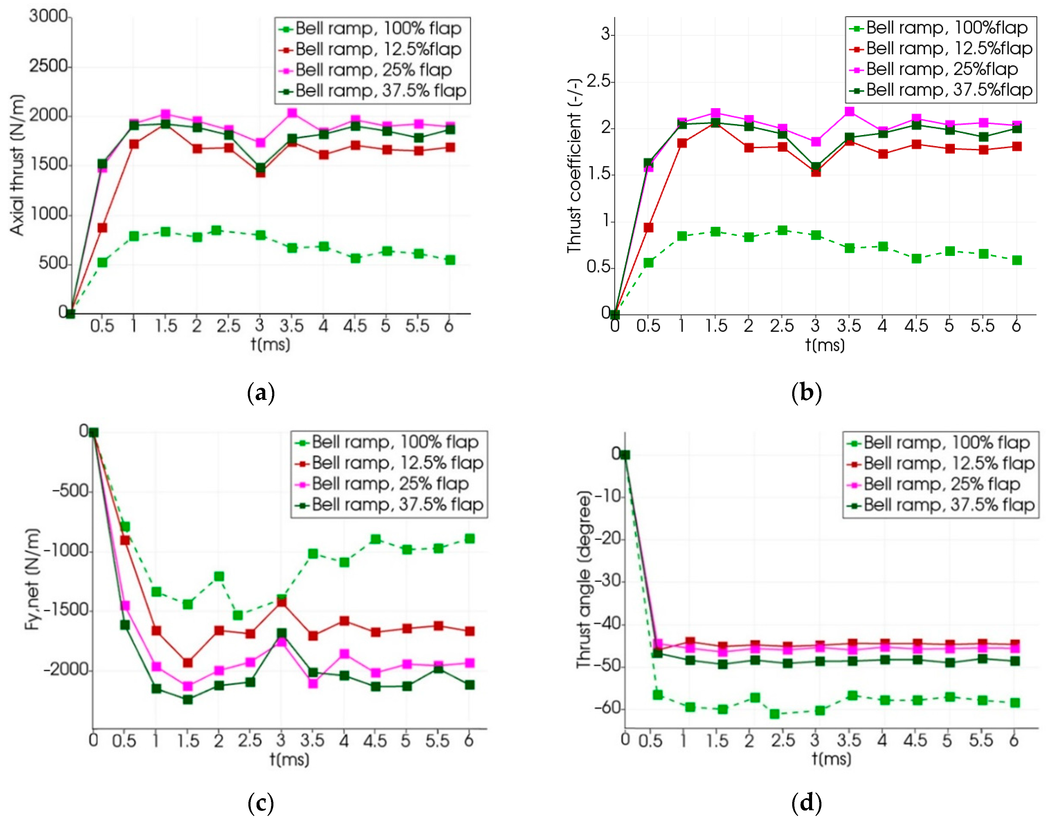
3.2.2. Analysis of Propulsion Performance of Bell-Shaped SERNs with Different Flap Lengths

The modification of a SERN ramp’s shape can generate different flow separation patterns. Figure 16a illustrates a distinct separation pattern RSS(flap) caused by the ramp’s modification. Short flap configurations should exhibit the same flow patterns in normal situations. However, in the short flap configurations, the excessive long flaps are removed, preventing the jet from reattaching to the flap. As a result, the flow exhibits the RSS(SERN) state, as depicted in Figure 16b. When comparing Figure 16b to the flow separation pattern of the conical-shaped configuration in Figure 13b, the bell-shaped profile leads to a larger separation bubble on the ramp and, therefore, results in a weaker adhesion force. As a consequence, after reattaching to the ramp, the jet briefly but significantly separates from the ramp. This stream jet bounce is described in Figure 17 as the bounce phenomenon. From both Figure 17a,b, it can be observed that the jet flow reattaches on the ramps’ rare part at t = 2 ms, generating a closed separation bubble. This separation bubble soon disappears at t = 3 ms in Figure 17c,d. Figure 17d clearly indicates that ambient fluid enters into the nozzle. The stream then rapidly reattaches again at t = 4 ms. The whole process occurs within only 2 ms.

The green dashed lines in Figure 18a–d depict the propulsion performance of the bell-shaped 100% flap length configuration in the RSS(flap) state. A longer reattachment speed is observed when it transitions to the RSS(flap) state. The conversion of RSS(flap) is not completed until 6 ms. The bell-shaped 100% flap length configuration in RSS(flap) exhibits a similar axial thrust in the steady state, but generates a larger vertical thrust than the original configuration of the RSS(SERN) state, leading to a thrust angle over −60°. Despite the distinct separation patterns between the conical and bell-shaped 100% flap length configurations, when compared with the thrust values before reattachment, a larger total thrust appears in the bell-shaped configuration, demonstrating the positive effect of the bell-shaped ramp modification in the 100% flap length configuration.

The relationship between the long flap configuration and short flap configuration from Figure 18a–c is similar to the relationship in Figure 14a–c. Compared to the long flap configuration, the short flap configurations exhibit higher thrust magnitudes, indicating that the effect of modifying the lengths of the flaps is more pronounced than modifying the ramp. A change in the ramp profile acts minorly yet variedly in short flap configurations. The bell-shaped 25% flap length configuration maintains a similar value in terms of both the axial and vertical thrust. However, the bell-shaped 12.5% flap length configuration experiences a decrease in axial and vertical thrust, denoting a decrease in the total thrust. Conversely, the bell-shaped 37.5% flap length configuration shows an increase in axial and vertical force.

However, the thrust angle behaves oppositely. In Figure 18d, the bell-shaped 100% flap length configuration exhibits a smaller thrust angle of around −60° throughout the entire simulation, while the short configurations exhibit a consistent thrust angle, around −45°, similar to the behavior of conical short flap length configurations.

Moreover, Figure 18a–d all show a scattered data distribution compared to the conical-shaped configurations, signifying a distinct and indirect impact of modification. The data also exhibit a bounce phenomenon in short flap configurations from 2.5 ms to 4 ms, also corresponding to the time described in Figure 17a–f. During this period, the axial thrust, axial propulsion coefficient, and vertical thrust all decrease due to this phenomenon. However, the axial and vertical thrust decrease by a certain proportion with time, maintaining the thrust angle as approximately unchanged.

Analysis of Propulsion Performance in RSS State between Conical-Shaped and Bell-Shaped Configurations with Equal Flap Length

This study further explores the comparison between conical-shaped and bell-shaped configurations with the same flap length. The choice of 25% flap length configurations is made due to their generation of similar flow patterns and improved axial thrust performance.

An analysis of Figure 19a,b highlights that the bell-shaped 25% flap length configuration showcases a slightly elevated axial thrust and axial propulsion coefficient. However, a bounce phenomenon occurring between 2.5 ms and 4 ms introduces a fluctuation in the bell-shaped configuration. Upon comparison, a similar, albeit slighter, bounce phenomenon emerges in the conical-shaped configuration within the same period. This suggests that reattachment effects commonly encounter bounce phenomena, but no significant variations in reattachment times.

Figure 19c depicts the larger vertical thrust magnitude of the bell-shaped configuration. The difference between each configuration at 6 ms, representing the steady state, is approximately −150 N/m. The greater axial and vertical thrust magnitudes indicate a positive effect of bell-shaped modifications. Nonetheless, the thrust increment is primarily in the vertical direction, exacerbating the negative downside force. Consequently, this leads to an approximately −2% increment in the thrust angle after modification, as depicted in Figure 19d.

In summary, from Section 3.2.2, it can be observed that a more prominent bounce phenomenon, the potential for alterations in flow patterns, and varying impacts on propulsion performance with different flap lengths due to bell-shaped modifications. The effect of modifying the ramp to a bell-shaped profile is less pronounced than the impact of shortening the flap.

4. Conclusions

This study is grounded in the utilization of the open-source program OpenFOAM. It serves as a foundational research endeavor, aiming to thoroughly explore the behavior of SERNs in static conditions characterized by an under-designed NPR (over-expansion conditions), spanning from startup to a steady state. The primary focus is on understanding the fundamental flow phenomena and propulsion performances in this condition. Additionally, the study evaluates the influence of two pivotal geometric parameters: the flap length and the ramp profile. The conclusions derived from this study can be categorized as follows:

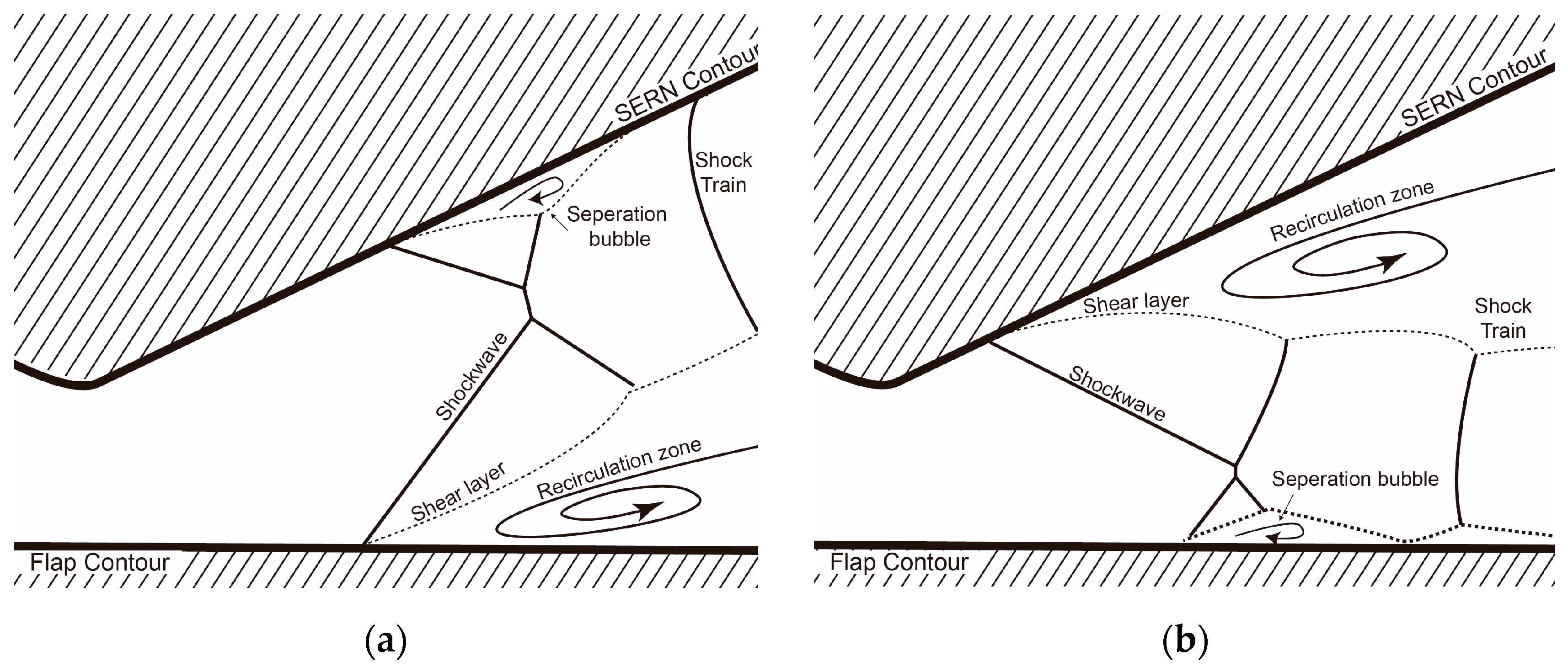
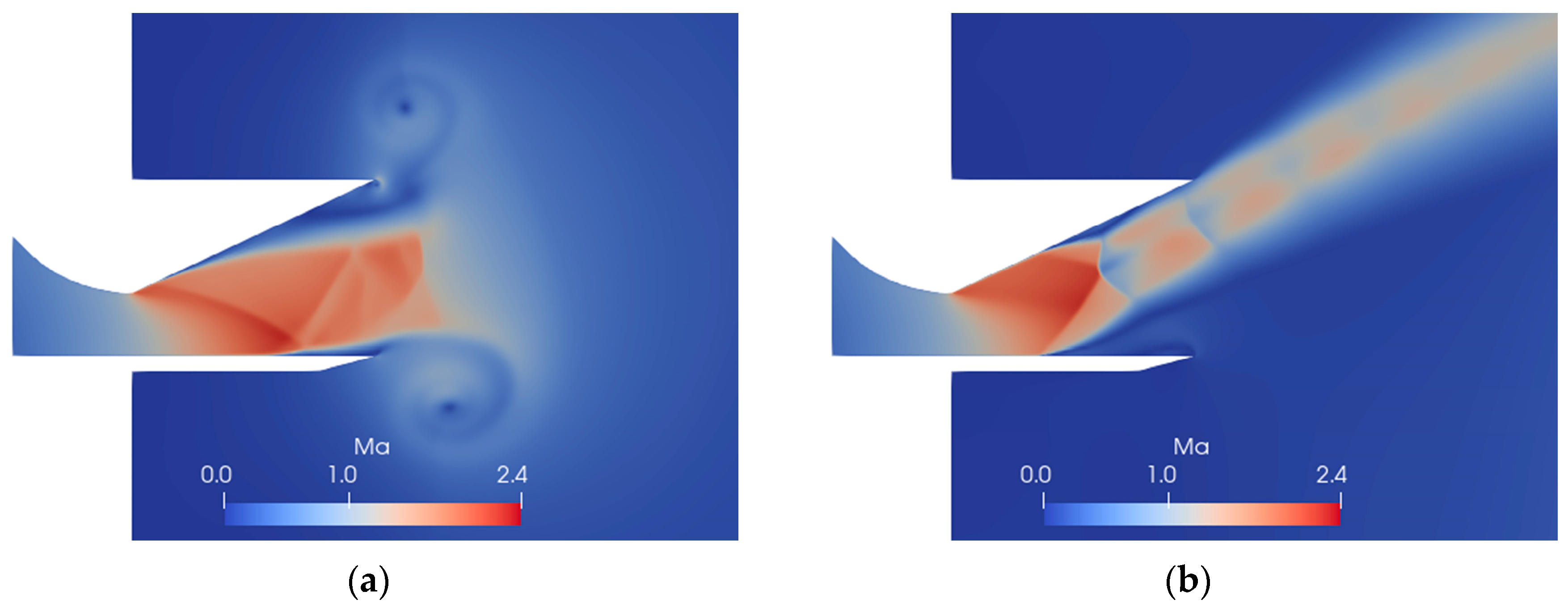
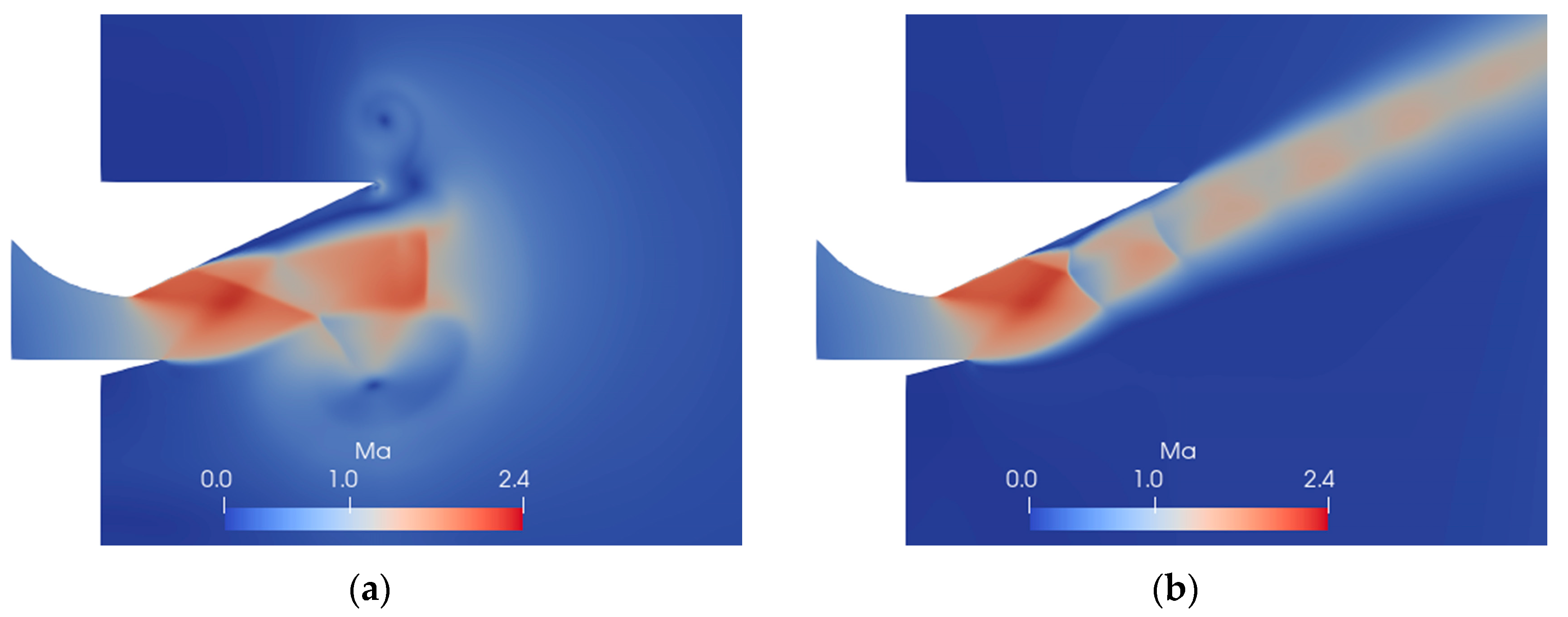
• The SERN configurations investigated in this research universally initiate with an FSS state, a consequence of the shockwave originating from the throat. This FSS state, while transient in nature under static conditions, evolves into a more stable RSS pattern due to the influence of viscous effects. Comparatively, the FSS state exhibits an elevated axial thrust and axial thrust coefficient and diminished vertical thrust magnitude and thrust angle magnitude, in contrast to the RSS state.
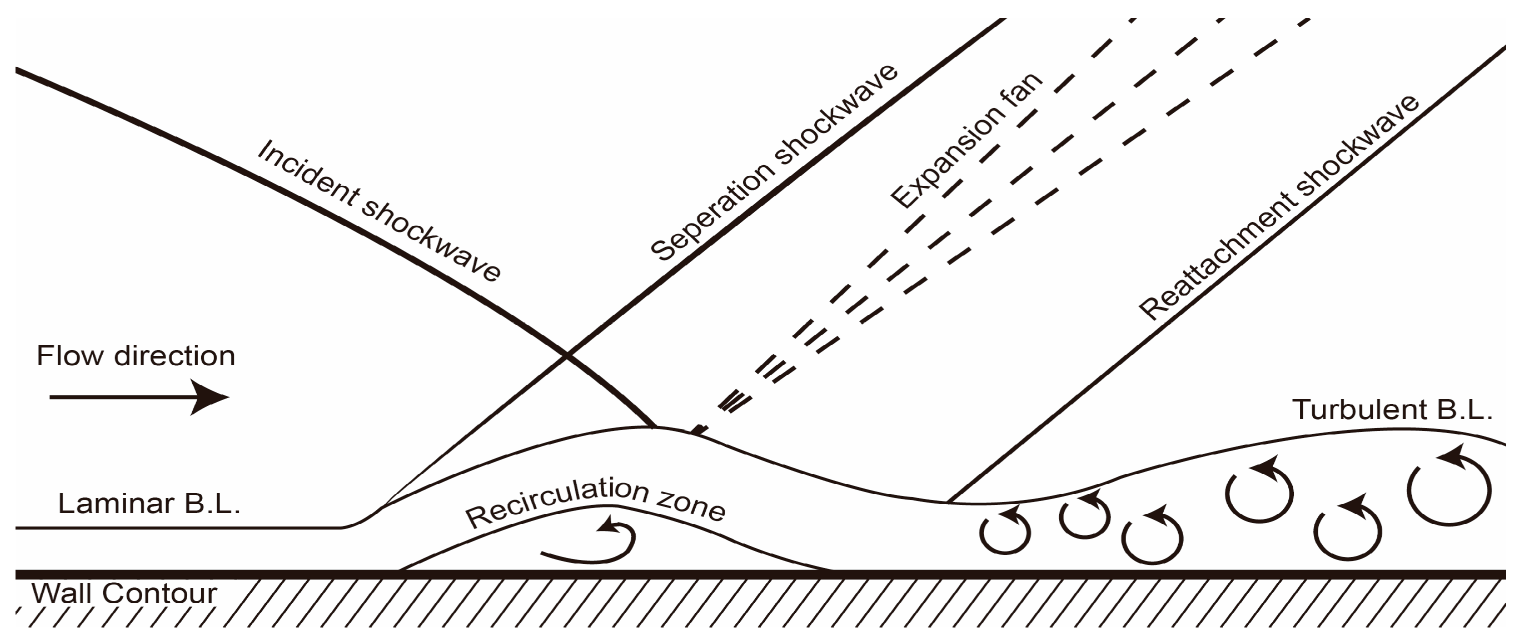
• In the static startup phase, a shockwave originates from the upper wall of the throat. Then, the shockwave occurs on the flap wall if the flap’s length permits; otherwise, it engages with the separation vortex. In cases where the shockwave interacts with the flap wall, this event characterizes the typical “incident shockwave”.
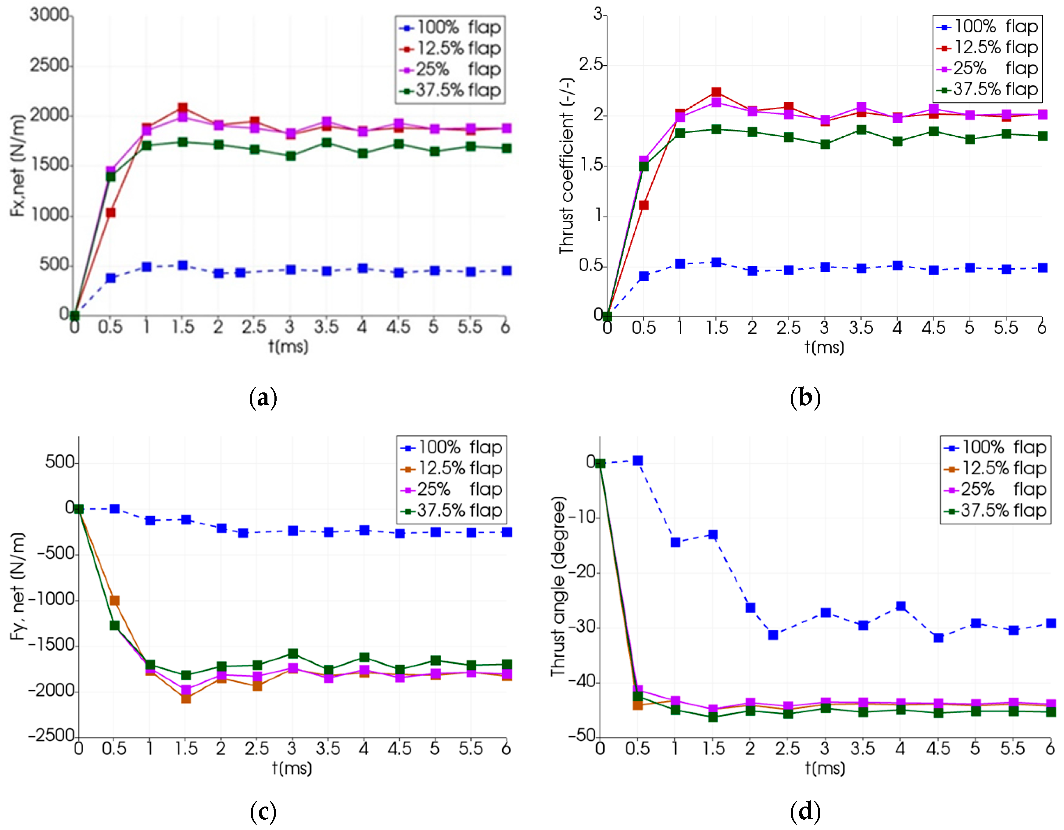
• The modified short flap configurations demonstrate accelerated separation speeds when compared to the original long flap configuration due to the emergence of a detachment vortex. A shorter flap is able to preclude backflow region creation and leads to a phenomenon akin to the attitude compensation seen in aerospike engines. Additionally, the total thrust is augmented, primarily due to an enlargement in the horizontal projection area of the thrust exit. However, this augmentation primarily amplifies the vertical net thrust and the thrust angle, with a 25° ramp potentially resulting in thrust angles of around −45°.
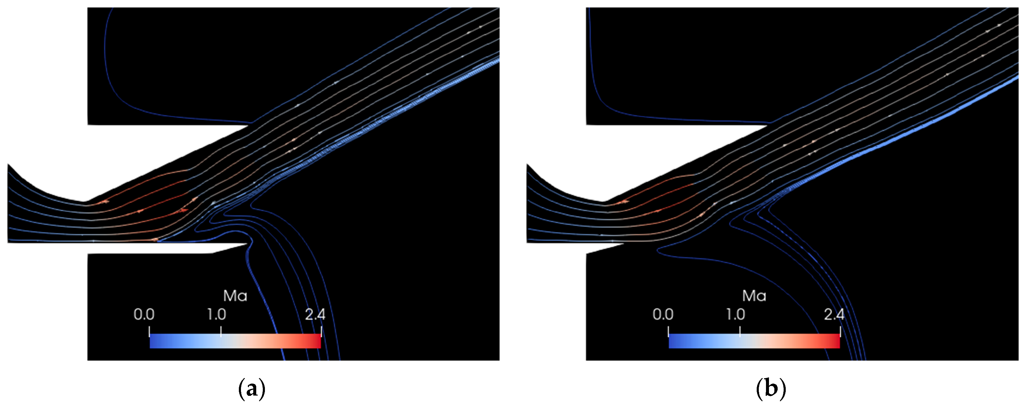
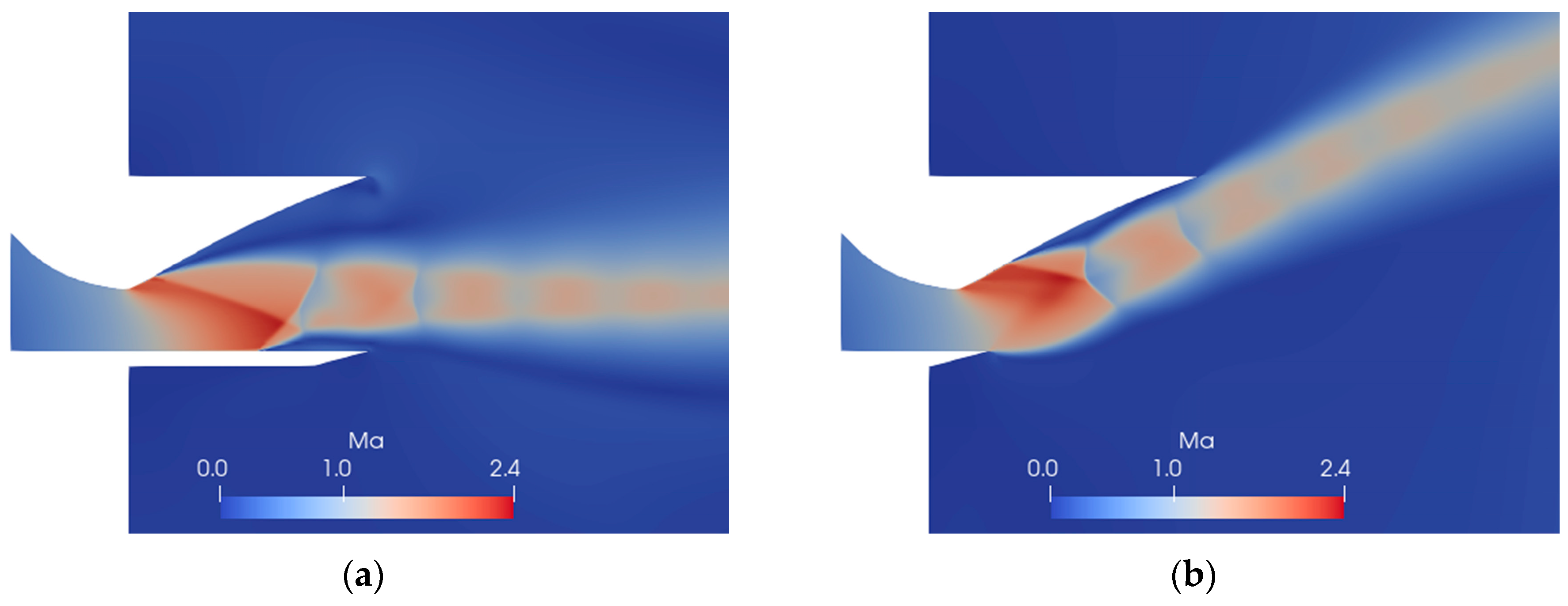
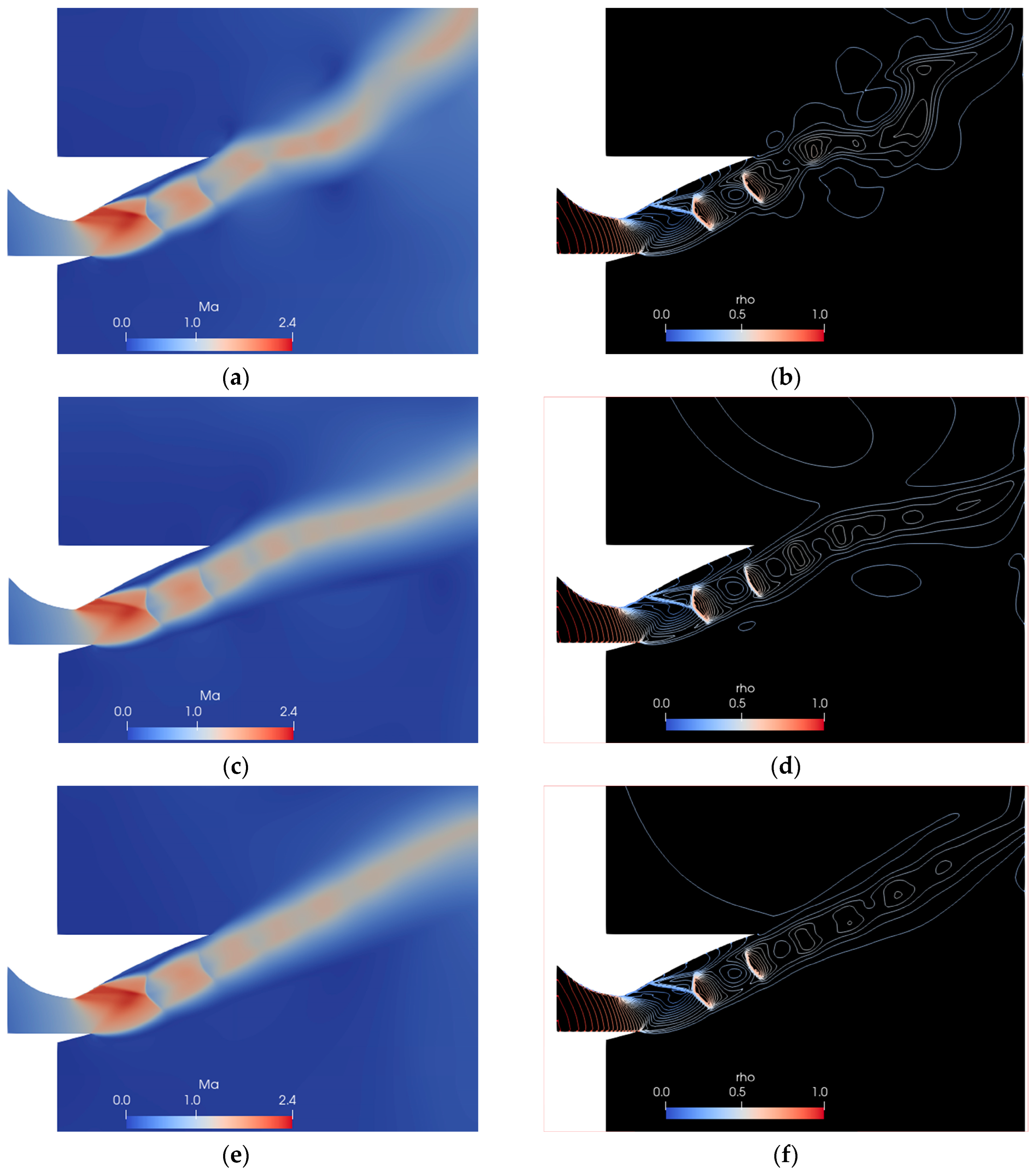
• Modifying the ramp profiles within this study yields three significant outcomes: Firstly, it is observed that altering the ramp profile can induce changes in the flow patterns during the steady state. Secondly, the introduction of a bell-shaped ramp profile tends to generate a larger separation bubble, particularly evident when the RSS(SERN) separation pattern occurs. Thirdly, while both conical-shaped and bell-shaped ramps display instances of jet bounce phenomena, the bell-shaped ramps exhibit a more pronounced bounce phenomenon.
• Both modifications involving shortening the flap and adjusting the bell-shaped ramp manifest similar effects, leading to an enhanced total thrust in over-expansion conditions. Nonetheless, most of the thrust enhancement is directed vertically. Furthermore, it is worth noting that flap shortening exhibits a more pronounced effect compared to the bell-shaped modification.

As preliminary research to study the effect of SERN geometries, this study mostly used traditional manners to establish and analyze the cases. Looking forward, in the future, studies will concentrate on applying systematic and efficient methods to conduct geomatic optimization, such as Method Constructal Design. More performance indicators should be added to such study to show not only thrust performance, but also a stability indicator to better depict the various effects of geometric variations. More external flow conditions should also be added to this studiy, not only limited to static conditions. Further holistic cases and analyses can be expected in future studies.

References

1. Seleznev, R.K. History of Scramjet Propulsion Development. In Proceedings of the Journal of Physics: Conference Series, Moscow, Russia, 21–24 November 2017; Institute of Physics Publishing: Bristol, UK, 4 May 2018; Volume 1009. [Google Scholar]
2. Drummond, J.P.; Bouchez, M.; Mcclinton, C.R. Chapter 1: Overview of NATO Background on Scramjet Technology; NATO Science and Technology Organization: Laspezia, Italy, 2010. [Google Scholar]
3. Urzay, J. Annual Review of Fluid Mechanics Supersonic Combustion in Air-Breathing Propulsion Systems for Hypersonic Flight. Annu. Rev. Fluid Mech. 2018, 50, 593–627. [Google Scholar] [CrossRef]
4. Li, R.; Xu, J.; Yu, K.; Lv, Z.; Cheng, K. Design and Analysis of the Scramjet Nozzle with Contact Discontinuity. Aerosp. Sci. Technol. 2021, 113, 106695. [Google Scholar] [CrossRef]
5. Yu, Y.; Xu, J.; Mo, J.; Wang, M. Principal Parameters in Flow Separation Patterns of Over-Expanded Single Expansion Ramp Nozzle. Eng. Appl. Comput. Fluid Mech. 2014, 8, 274–288. [Google Scholar] [CrossRef]
6. Yu, K.; Chen, Y.; Huang, S.; Xu, J. Inverse Design Method on Scramjet Nozzles Based on Maximum Thrust Theory. Acta Astronaut. 2020, 166, 162–171. [Google Scholar] [CrossRef]
7. Yu, K.; Xu, J.; Lv, Z.; Song, G. Inverse Design Methodology on a Single Expansion Ramp Nozzle for Scramjets. Aerosp. Sci. Technol. 2019, 92, 9–19. [Google Scholar] [CrossRef]
8. Ridgway, A.; Sam, A.A.; Pesyridis, A. Modelling a Hypersonic Single Expansion Ramp Nozzle of a Hypersonic Aircraft through Parametric Studies. Energies 2018, 11, 3449. [Google Scholar] [CrossRef]
9. Houghton, E.L.; Carpenter, P.W.; Collicott, S.H.; Daniel, T. Valentine Aerodynamics for Engineering Students, 6th ed.; Elsevier: Amsterdam, The Netherlands, 2016; ISBN 9780080966328. [Google Scholar]
10. Ligrani, P.M.; McNabb, E.S.; Collopy, H.; Anderson, M.; Marko, S.M. Recent Investigations of Shock Wave Effects and Interactions. Adv. Aerodyn. 2020, 2, 4. [Google Scholar] [CrossRef]
11. Gaitonde, D.V. Progress in Shock Wave/Boundary Layer Interactions. Prog. Aerosp. Sci. 2015, 72, 80–99. [Google Scholar] [CrossRef]
12. OpenFOAM v6 User Guide. Available online: https://doc.cfd.direct/openfoam/user-guide-v6/contents (accessed on 31 July 2021).
13. Kurganov, A.; Noelle, S.; Petrova, G. Semi-Discrete Central-Upwind Schemes for Hyperbolic Conservation Laws and Hamilton-Jacobi Equations. Soc. Ind. Appl. Math. 2001, 23, 1461–1488. [Google Scholar]
14. Greenshields, C.J.; Weller, H.G.; Gasparini, L.; Reese, J.M. Implementation of Semi-Discrete, Non-Staggered Central Schemes in a Colocated, Polyhedral, Finite Volume Framework, for High-Speed Viscous Flows. Int. J. Numer. Methods Fluids 2010, 63, 1–21. [Google Scholar] [CrossRef]
15. Shieh, T.H.; Li, M.R.; Li, Y.T. Study of New Accurate Supplementary Energy Modeling With Multi-Components Based on Newly Developed High Resolution Scheme. Int. Commun. Heat Mass Transf. 2019, 107, 121–140. [Google Scholar] [CrossRef]
16. Nessyahu, H.; Tadmor, E. Non-Oscillatory Central Differencing for Hyperbolic Conservation Laws. J. Comput. Phys. 1990, 87, 408–463. [Google Scholar] [CrossRef]
17. Gruhn, P. Einfluss Einer Heckklappe Die Düsenströmung Im Hyperschall. Ph.D. Dissertation, Rheinisch-Westfälischen Technischen Hochschule Aachen, Aachen, Germany, 2004. [Google Scholar]
18. Naveen Kumar, K.; Gopalsamy, M.; Antony, D.; Krishnaraj, R.; Viswanadh, C.B.V. Design and Optimization of Aerospike Nozzle Using CFD. In Proceedings of the IOP Conference Series: Materials Science and Engineering, Coimbatore, India, 3–4 March 2017; Institute of Physics Publishing: Bristol, UK, 16 October 2017; Volume 247. [Google Scholar]
19. Rao, G.V.R. Exhaust Nozzle Contour for Optimum Thrust. J. Jet Propuls. 2012, 28, 377–382. [Google Scholar] [CrossRef]
20. Lee, C.; Choi, K.; Kim, C.; Han, S. Computational Investigation of Flow Separation in a Thrust-Optimized Parabolic Nozzle during High-Altitude Testing. Comput. Fluids 2020, 197, 104363. [Google Scholar] [CrossRef]
21. Niezdodka, J. Druckverteilungsmessungen zur Simulation der Interferenz des Triebwerksstrahls Auf das Heck der Sänger-Unterstufe; DLR-WT-WK: Cologne, Germany, 1993. [Google Scholar]
22. Esch, T.; Bauer, A.; Rick, H. Simulation and Nozzle/Afterbody Integration of Hypersonic Propulsion Systems. Z. Flugwiss. Weltraumforsch. 1995, 19, 19–28. [Google Scholar]
23. Weinand, K. Numerische Berechnung der Strömung in Einem Windkanalheckteilmodell Mit Einem Finite-Elemente-Verfahren; University Aachen: Aachen, Germany, 1994. [Google Scholar]
Figure 1. The schematic diagrams of the mesh verification 1. (a) The geometry and the surface pressure acquisition area (red line) and (b) the computational domain and the main boundary names.
Symmetry 16 01044 g001
Figure 2. The schematic diagrams of the mesh verification 2. (a) The geometry and the surface pressure acquisition area (red line) and (b) the computational domain and the main boundary names.
Symmetry 16 01044 g002
Figure 3. The schematic diagrams of the short flap research models of conical (a) 37.5%; (b) 25%; and (c) 12.5% flap length configurations. The geometric changes are denoted by red arrows.
Symmetry 16 01044 g003
Figure 4. The schematic diagrams of the bell-shaped research models with (a) 100%, (b) 37.5%, (c) 25%, and (d) 12.5% flap length configurations. The differences between each configuration are highlighted by red words.
Symmetry 16 01044 g004
Figure 5. The diagrams demonstrate the (a) coarse; (b) medium; and (c) fine meshes around the scramjet device (core area).
Symmetry 16 01044 g005
Figure 6. The diagrams demonstrate the (a) coarse mesh around the nozzle; (b) coarse mesh around the flap tip; (c) medium mesh around the nozzle; (d) medium mesh around the flap tip; (e) fine; mesh around the nozzle; and (b) fine mesh around the flap tip. The comparison between (a,c,e) demonstrates the overall mesh situation around the nozzle (core area). The comparison between (b,d,f) rather indicates the difference of densification around the walls.
Symmetry 16 01044 g006
Figure 7. The flow reattaches on the different walls and forms (a) RSS(SERN) phenomena and (b) RSS(flap) phenomena, respectively.
Symmetry 16 01044 g007
Figure 8. A comparison between the experimental data and (a) the results from the different mesh resolutions and (b) the most optimal result and the historical simulation results in mesh verification case 1.
Symmetry 16 01044 g008
Figure 9. Comparisons between the experimental data and (a) the results from the different mesh resolutions and (b) the most optimal result and the historical simulation result [5] in mesh verification case 2.
Symmetry 16 01044 g009
Figure 10. The Mach number contours of mesh verification 2 at (a) t = 0.4 ms, indicating the flow pattern in the early flow development phase; (b) t = 6 ms, indicating the flow pattern of the steady state.
Symmetry 16 01044 g010
Figure 11. Incident shockwave, classical shockwave, and boundary interaction (SWBLI) phenomena.
Symmetry 16 01044 g011
Figure 12. The graphs of the relationships between time and (a) axial thrust; (b) thrust coefficient; (c) Fy, net (vertical thrust); and (d) thrust angle in mesh verification 2.
Symmetry 16 01044 g012
Figure 13. The Mach number contours of the short flap configuration (conical, 12.5% flap length configuration for example) at (a) t = 0.4 ms and (b) t = 6 ms.
Symmetry 16 01044 g013
Figure 14. Variations in (a) axial thrust; (b) thrust coefficient; (c) vertical thrust (lift); and (d) thrust angle with flap length.
Symmetry 16 01044 g014
Figure 15. The streamline diagrams indicate the flow that passes through (a) the long flap configuration with the air entering the nozzle, resulting in a backflow area; and (b) the short flap configuration (using 12.5% flap length as a representative) without a backflow area.
Symmetry 16 01044 g015
Figure 16. The Mach number contours of the bell-shaped 100% flap length configuration at (a) t = 0.4 ms, which generates a different flow separation pattern, RSS(flap), after modifying from a conical to a bell-shaped ramp; and (b) t = 6 ms, which remains the same RSS state after the modification.
Symmetry 16 01044 g016
Figure 17. The bell shape causes the most significant bounce phenomenon. The pictures are contour diagrams of 12.5% flap length configuration for (a) Mach at t = 2 ms; (b) density at t = 2 ms; (c) Mach at t = 3 ms; (d) density at t = 3 ms; (e) Mach at t = 4 ms; and (f) density at t = 4 ms.
Symmetry 16 01044 g017
Figure 18. Variations in (a) axial thrust; (b) axial propulsion coefficient; (c) vertical force; and (d) thrust angle of bell-shaped configuration with flap lengths.
Symmetry 16 01044 g018
Figure 19. Comparisons of (a) axial thrust; (b) axial propulsion coefficient; (c) vertical thrust; and (d) thrust angle in conical-shaped and bell-shaped 25% flap length configurations.
Symmetry 16 01044 g019