Article

Enhancing Symmetry and Memory in the Fractional Economic Growing Quantity (FEGQ) Model

by
Azedine Ouhmid
1,†,
Karim El Moutaouakil
1,*,†,
Fatima Belhabib
1,† and
Alina-Mihaela Patriciu
2,*,†
1
Laboratory of Engineering Sciences, Multidisciplinary Faculty of Taza, Sidi Mohamed Ben Abdellah University, Taza 35000, Morocco
2
Department of Mathematics and Computer Sciences, Faculty of Sciences and Environment, Dunărea de Jos University of Galaţi, 800201 Galaţi, Romania
*
Authors to whom correspondence should be addressed.
These authors contributed equally to this work.
Symmetry 2024, 16(8), 1057; https://doi.org/10.3390/sym16081057
Submission received: 27 June 2024 / Revised: 31 July 2024 / Accepted: 13 August 2024 / Published: 16 August 2024

Abstract

:
In this paper, we present a novel approach to inventory management modeling, specifically tailored for growing items. We extend traditional economic growth quantity (EGQ) models by introducing the fractional economic growing quantity (FEGQ) model. This new approach improves the model’s symmetry and dynamic responsiveness, providing a more precise representation of the changing nature of inventory items. Additionally, the use of fractional derivatives allows our model to incorporate the memory effect, introducing a new dynamic concept in inventory management. This advancement enables us to select the optimal business policy to maximize profit. We adopt the fractional derivative in terms of Caputo derivative sense to model the inventory level associated with the items. To analytically solve the (FEGQ) model, we use the Laplacian transform to obtain an algebraic equation. As for the logistic function, known for its symmetrical S-shaped curve, it closely mirrors real-life growth patterns and is defined using fractional calculus. We apply an iterative approximation method, specifically the Adomian decomposition method, to solve the fractional logistic function. Through a sensitivity analysis, we delve for the first time into the discussion of the initial weights, which have a massive impact on the total profit level. The provided numerical data indicate that the firm began with a favorable policy. In the following years, several misguided practices were implemented that led to a decrease in profitability. The healing process began once again by selecting more effective strategies.

1. Introduction

The economic order quantity (EOQ) model is a fundamental inventory management tool used by businesses to determine the optimal order size that minimizes the total costs associated with inventory, including ordering and holding costs. Harris [1] made the first inventory model in the second half of the 1800s, which was the beginning of the field of inventory modeling. Later, Wilson [2] built on it by using a mathematical model to come up with methods for obtaining economic order quantities. The model is known as the classic EOQ. The classic EOQ model is based on certain assumptions, such as a constant demand rate, a fixed ordering cost, and a steady holding cost per unit. Despite its simplicity, the EOQ model has been widely used in various industries to streamline inventory processes and reduce costs. However, the utility and dynamic nature of real-world systems often deviate from these assumptions. Traditional EOQ models may not adequately capture the complexities of growing items, fluctuating demand, or time-dependent changes in inventory levels (ILs). To address these limitations, advanced mathematical techniques, such as fractional calculus, have been integrated into inventory modeling.
Fractional calculus is a novel area of applied analysis that works with complex or real derivatives of any order. By extending the concepts of differentiation and integration to non-integer orders, this approach offers a more thorough foundation for comprehending dynamic systems. In contrast to integer-order calculus, fractional calculus, which was once thought to be abstract, developed quickly in the 19th century and provided a more accurate explanation of natural and practical processes. Since then, numerous academic fields, including mathematics, economics, physics, and engineering, have given it serious consideration [3,4,5,6,7]. Fractional calculus is a useful tool because it can take into account the memory effect, which is frequently disregarded in models that rely on differential equations of integer order. Fractional calculus is a framework that generalizes integer-order calculus and better reflects the complexities of dynamic systems, improving our knowledge and modeling abilities in a variety of domains. A notable advancement in inventory modeling came with the introduction of fractional calculus. Pioneered by Das and Roy in 2015 [8], fractional calculus has been utilized to extend EOQ models, incorporating time-varying demand and memory effects through fractional differential equations. Two years later (2017), Das and Roy [9] made a further attempt, providing an appropriate mathematical model for inventory management using fractional calculus while the production rate, as well as the demand, is considered constant. In 2018, Pakhira et al. [10] introduced a fractional approach to a classical inventory model with quadratic demand rates. Unlike in the previous models ([8,9]), in their study, they delve into various approaches and explore the macroscopic behavior of the model across a spectrum of memory ranges, from long to low. This was the first time the memory effect was considered in an inventory model. In the same year, Pakhira et al. [11] developed another model that generalizes the inventory model. Three types of generalization with fractional computation have been proposed: in the first model, only demand rates change fractionally; in the second model, the demand ratio and the stock level are extended with the identical fractional index; in the third model, the rate of demand and the level of inventories have been aggregated, if necessary, in the same fractional index. All fractional models are governed by the Caputo fractional order derivative. Fractional calculus concepts were applied to the inventory control problem in 2020 by Rahaman et al. [12]. During their research, they examined many scenarios and improved the fractional-order economic production quantity (EPQ) model by incorporating a uniform demand and production rate, as well as a uniform demand, production rate, and deterioration. The problem is solved by using the rational approximation approach of the generalized Mittag-Leffler functions, which involves different poles. In the same year (2020), Das et al. [13] proposed a fractional-order generalized economic order quantity (EOQ) model with constrained storage capacity, wherein demand varies inversely with unit production cost. They employed geometric programming techniques to obtain the optimal solution for the fractional-order EOQ model. In 2021, Rahaman et al. [14] studied the impacts of memory and learning due to experiences on the decision-making process. The demand is modeled as a function of price. Fractional calculus is integrated into the model as an effective tool to study the memory effect; on the other side, fuzzification is used as a tool to represent experience-based learning. Later (2022), attempting to find a more generalized version of the classical EOQ, Rahaman et al. [15] utilized fractional calculus concepts to address inventory control problems under fuzzification. Two main impacts have been studied in this research: the effect of uncertainty, which is represented by the notion of fuzziness, and system memory, which is represented by the fractional derivative. These advancements highlight the potential of fractional calculus to improve the robustness and accuracy of inventory models, especially in cases involving dynamic and non-linear processes. Despite the substantial benefits of fractional calculus in creating more precise and adaptive inventory models, its application to the EOQ model for growing items, known as the Economic Growing Quantity (EGQ) model, remains unexplored. Since Jaafar [16] pioneered the EGQ model, all studies have used the first differential equation to describe its parameters, such as feeding cost, holding cost, and inventory level. This unexplored research opportunity represents a significant gap, as harnessing the sophisticated mathematical framework of fractional derivatives could lead to the development of a fractional economic order quantity (FEGQ) model specifically tailored for growing items. This innovative approach aims not only to enhance the precision of inventory management for dynamically growing items, but also to pave the way for a new paradigm in the field, addressing complex growth dynamics and offering transformative potential for modern inventory strategies. Unfortunately, the models considered in quantitative economic growth models implement an integer derivative to describe item growth and inventory levels. In addition, it is well known that the rate of temporal change of integer derivatives is predetermined by the characteristic of differentiable functions of time only in extremely close proximity to the current moment. Consequently, marginal output is expected to fluctuate momentarily as input levels change. Consequently, the effects of dynamic memory are not observed in the conventional model.
In this paper, we introduce a fractional economic order quantity (FEGQ) model for growing products to account for the memory effect. In fact, in the fractional derivative, the rate of change is influenced by all the points in the interval under consideration, thus incorporating the system’s memory, and the fractional order is physically treated as a storage indicator. It can therefore overcome system forgetting. To build the FEGQ model, we first describe the logistic evolution of growth using β -fractional logistics. In addition, we describe the dynamics of IL using an α -fractional differential equation. Next, the evolution of the holding cost is described using a δ -fractional differential equation. To explain the total profit equation, we apply the Adomian decomposition method to reveal the growth function equation. Next, we use the Laplacian transformation to explicitly determine the IL equation. In this sense, three essential cases of study are examined: (a) short-term memory of holding costs, (b) short-term memory of inventory levels, and (c) long-term memory of inventory levels and holding costs. We used the proposed model to determine the optimal length of the consumption period and the maximum total profit expected in the context of the chicken breed. The experiment was based on real-life data. The results obtained were compared with those obtained by conventional EOQ models.
The main contributions of this work are summarized as follows:
  • Memory augmentation of the EGQ model by introducing the fractional logistic function to the EGQ problem to describe item growth;
  • Memory augmentation of the EGQ model by introducing the fractional IL to the EGQ problem;
  • Memory augmentation of the EGQ model by introducing the fractional version of the total profit that implements previous fractional dynamic models;
  • Application of the resulting fractional economic growing quantity model, considering different fraction order, to estimate an optimal policy for a particular breed of chickens using the Adomian decomposition method.
This paper is organized as follows: Section 2 presents the methodology adopted in the paper. Section 3 gives the fractional calculus basics. Section 4 presents the classical economic growth quantity model. Section 5 introduces the proposed fractional economic growth quantity model. Section 6 provides several experimental tests of the proposed model. Section 7 gives some conclusions, limitations, and future scope of this research.

2. Methodology

In this section, we give the main steps adopted to build our model; see Figure 1.
In the following, we shall give the idea behind each component:
First, we recall the main important components of the classical EGQ model that implement simple logistic and describe the IL using a first-order differential equation. When generalizing this model, the following assumptions are adopted:
A1
The item’s annual demand remains consistent over time.
A2
The shortages are prohibited.
A3
The items ordered can grow before being slaughtered, and the cost of feeding them depends on the weight gained.
A4
The items with poorer quality and the items disposed of due to mortality are not considered.
Second, we extend this model memory by introducing fractional logistic (to describe the evolution of the item’s growth) and the fractional order of IL.
Third, to make the fractional total profit explicit, we use the Adomian decomposition method and the Laplacian operator. This allows for distinguishing three main study cases that need to be known: short growth memory, long growth and IL memory, and short IL memory.
Fourth, to illustrate the performance of the proposed method, we use the FEGQ model to describe the evolution of breeds of chickens and to estimate the optimal duration of the maturation process, the length of the consuming period, and the quantity of newly hatched chicks requested at each breeding cycle.

3. Fractional Calculus Basics

In this section, we briefly review the fractional derivative of Riemann–Liouville and Caputo. In addition, we give the principle of the Adomian decomposition method.

3.1. Fractional Derivative of Riemann–Liouville and Caputo

Within this part, we are going to provide two significant definitions: the Riemann–Liouville (RL) definition and the Caputo–Fabrizio (CF) definition. In addition, we shall incorporate the fractional Laplace transform method into the construction of this work. Before proceeding, we outline the definition of the gamma function.
The gamma function is a mathematical tool that takes the place of the factorial operator to extend factorials for non-integer numbers and is written as follows:
Γ ( α ) = 0 + r α 1 e r d r .
where α is non-integer number.
The RL integral is defined as follows:
I r α α R l g ( r ) = 1 Γ ( α ) a r ( r s ) α 1 g ( s ) d s r R .
The fractional derivative, known as the RL fractional derivative of any order, is defined as
D r α α R l g ( r ) = 1 Γ ( n α ) d n d r n a r ( r s ) n α 1 g ( s ) d s r R .
The CF derivative is defined as
D r α α C g ( r ) = 1 Γ ( n α ) a r ( r s ) n α 1 g ( n ) ( s ) d s r R .
In this paper, we intend to generalize the EGQ model by introducing the fraction EGQ model that implements the CF derivative.

3.2. Laplace Transformation of the Fractional Derivative and Integral

The Laplace transform (LT) and its inverse constitute a powerful technique for solving linear differential equations that are difficult to solve directly. To this end, LT converts the differential equations into algebraic equations, which are often easier to solve [17]. In this section, we define the Laplace transform and some of its properties.
The Laplace transform of the function g ( t ) is defined as
Φ ( s ) = L ( g ( t ) ) = 0 + e s t g ( t ) d t ,
where s > 0 .
The inverse Laplace transform of a function Φ ( s ) is given by
L 1 ( Φ ( s ) ) = g ( t ) = + e s t Φ ( s ) d t .
The LT for integer numbers can be expressed as shown in Equation (5).
L g p ( t ) = s p Φ ( s ) k = 0 p 1 s p k 1 g k ( 0 )
The LT for non-integer numbers is given by the following equation:
L g α ( t ) = s α Φ ( s ) k = 0 m 1 s k g α k 1 ( 0 ) ( m 1 ) < α < m .
In Section 5.2, we shall implement Equation (4) to make the fractional IL explicit.

3.3. Principle of the Adomian Decomposition Method

Unlike in linear fractional equations, finding an exact solution to nonlinear fractional differential equations, such as the logistic function, poses a challenge. In his paper [18], West proposed an exact solution to the fractional logistic equation; unfortunately, his solution is valid only for α = 1 (see [19]). Consequently, an approximate method takes its place. To handle this problem, we utilize in this paper the Adomian decomposition method (ADM). In this method, the solution is assumed to be of the form i = 1 + v i . The idea of this iterative method is to decompose the fractional derivative operator D α by expressing it as a sum of simpler differential operators. In order to solve equations without the need for linearization, discretization, perturbation, or any other limiting assumptions, we employ an approach that involves dividing the problem into two distinct forms: linear and nonlinear. Adomian polynomials are employed to decompose the nonlinear expression, and a recursive iterative algorithm is employed to obtain the solution [20,21,22]. Next, we provide how to use Adomian polynomials to approximate the solution. Consider the following equation:
τ ( v ) + ρ ( v ) + η ( v ) h = 0 ,
where τ is the highest-order derivative, ρ is a linear differential operator, η represents the nonlinear terms, and h is a given function.
We apply τ 1 to Equation (7) and obtain
v = v 0 + τ 1 h τ 1 ρ ( v ) τ 1 η ( v ) .
The nonlinear operator in the equation is decomposed by an infinite series of polynomials; those polynomial terms are called the Adomian polynomials, and they are expressed as
η ( v ) = i = 1 + A i .
The Adomian polynomials can be calculated for all types of nonlinearities by using the following algorithm proposed by Adomian:
A n = 1 n ! · n λ n η i = 1 + v k · λ k λ = 0 n = 1 , 2 ,
By substituting in Formula (8) we obtain
i = 1 + v i = v 0 + τ 1 h τ 1 ρ i = 1 + v i τ 1 i = 1 + A i .
Iteratively, we determine the term of the sequence v n .
We are going to apply that to the fractional logistic function.

3.4. Kernel-Dependent Derivative

The derivative of a function x ( s ) with the help of the kernel k ( s s ) is given by:
d x ( s ) d s = a s k ( s s ) · g ( s ) d s
where g ( s ) is an integrable function of one variable.
To derive the concept of memory effect, we consider kernel function in terms of power law in the form k ( s s ) = ( s s ) ( α 2 ) Γ ( 1 α ) , the Equation (9) can be reduce to the form d ( x ( s ) ) d s = D s ( α 1 ) α ( g ( s ) ) .
The parameter α in fractional calculus governs the memory strength of the system. As α approaches 1, the system weakens in terms of memory, and when α tends to 1, the system becomes completely memory-less. A lower value of α signifies stronger memory retention within the system.

4. Classic EGQ Model

In this section, we present the fractional economic growth quantity (FEGQ) model, which generalizes the EOQ model based on the classical derivative.
In this section, we give the classical mathematical model that can be used to describe the evolution of the growing entities; Table 1 gives the list of symbols adopted in the paper. In this sense, we consider a scenario where a company purchases newborn animals, raises them, and subsequently slaughters and trades them in the marketplace. The organization aims to determine the optimal quantity of newborn animals to procure and the optimal day to butcher them in order to fulfill demand.
The general mathematical model implements two main terms (TC: Total Cost and TR: Total Revenue) described by Equation (10) [23].
Total Profit ( TP ) = TR TC .
In the following, we define the TR and different types of costs:
Total revenue: Given the selling price of an item as s, the total revenue equals
TR : total revenue = s . y · w 1 .
The total cost implements five kinds of cost: purchasing cost (PC), setup cost (SC), feeding cost (FC), holding cost (HC), and vaccination cost (VC).
Purchasing cost: At the start of the cycle, the corporation purchases y items at a cost of p per item, each with a starting weight of w 0 . Therefore, the purchase cost is
PC : the purchasing cost = p · y · w 0 .
Setup cost: This cost includes all expenses related to the procurement of inventories, as follows:
S C : The setup cost = K ,
where K is constant.
Feeding cost: It refers to the feeding expenses required for a newborn chick to reach maturity. Here, we employ the logistic function to illustrate the progression of weight over time, as follows:
d w ( t ) d t = λ · w ( t ) b · w 2 ( t ) , w ( 0 ) = m ,
where λ is the growth rate, A is the carrying capacity, and b = λ A . To make the feeding cost explicit, we solve Equation (11) and we obtain the following equation:
w ( t ) = A 1 + n · e λ t with n = A m m .
Using a simple analytical calculation, we can find the duration time t 1 needed to reach the targeted weight w 1 , as follows:
t 1 = ln 1 n · A w 1 1 / λ .
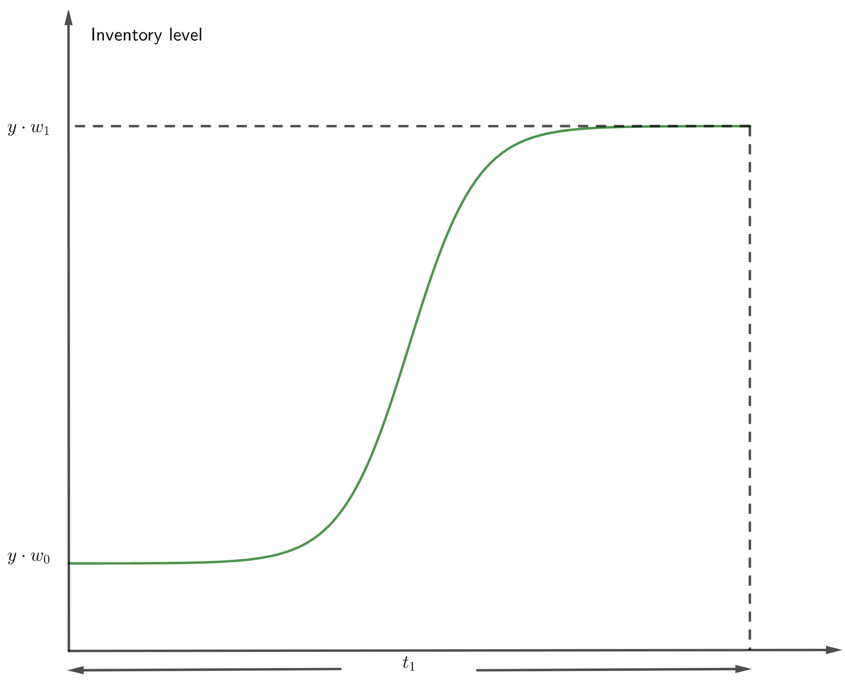
Figure 2 illustrates the progression of broiler chicken weight over time. In this regard, the weight first exhibits a modest increase, progressively gaining momentum until the hens attain the target weight.
Holding cost: This cost encompasses all expenses associated with holding items in inventory. Given H, the cost of holding a single unit, which is assumed to be constant in our model, the total holding cost is obtained by multiplying the IL by H. The inventory dynamic can be expressed by Equation (12).
d I ( t ) d t = N , I t 1 + T = 0 and I t 1 = y · w 1 .
By solving Equation (12), we obtain
I ( t ) = N · t t 1 + y · w 1 = N · t t 1 + D · T .
Therefore, we obtain
I ( t ) = N T + t 1 N · t .
Figure 3 depicts the duration of consumption. Once the newly hatched chickens reach the desired weight w 1 , they are slaughtered and prepared for consumption by consumers. The IL subsequently declines until it hits zero at time T.
Vaccination cost: It pertains to the expense of vaccinating each item at the start of the cycle.
V C = q · y .
Towards the end, the total profit equation of the system during the whole-time cycle is given by Equation (13).
T P U = s · y · w 1 p · y + c · y · 0 t 1 w t d t + K + h · y + H · T · y · w 1 2 + q · y .
To obtain the expected total profit by unit ( E [ T P U ] ), we divided T P by the cycle duration T, as follows:
E ( T P U ) = E ( T P ) T = T R S C P C H C F C V C T .
E [ T P U ] is given by Equation (14).
E ( T P U ) = s · N p · N w 1 + N · c 0 t 1 w t d t w 1 + K T + N · h w 1 + H · N · T 2 + q · N w 1 .
The maximum of the function E [ T P U ] , considering the variables T, can be obtained by solving the equation d E ( T P U ) d T = 0 . In this sense, we obtain
T * = 2 · K H · N and y * = T * · N w 1 .
In the coming section, we are going to generalize this model by describing different components using fractional calculus that take into account the memory effect [24].

5. Proposed Fractional Economic Growing Quantity (FEGQ)

To introduce our fractional economic growth quantity model, we introduce the fractional logistic function and the fractional IL. We then explain them using the Adomian decomposition method and the Laplacian transform operator.

5.1. Fractional Logistic Function to EGQ Problem

The first step towards generalizing the classic EGQ model is to describe item growth using fractional order to improve the accuracy of the classic model. The obtained model is given by the following Equation (16):
D β w ( t ) = λ · w ( t ) b · w 2 ( t ) , w ( 0 ) = m a n d b = λ A .
Since the model (16) is not linear, we turn to ADM as a solution approach [21].
Theorem 1.
The solution of Equation (16) has the form
w ( t ) = m + 1 Γ ( 1 + β ) λ · m b · m 2 t β + λ 2 · b · w 0 · λ · m b · m 2 Γ ( 1 + 2 β ) · t 2 β
Proof. 
We apply the operator I β , the inverse of the operator D β , to both sides of Equation (16), and using the initial condition, we obtain
w ( t ) = m + λ . I β ( w ( t ) ) b . I β w 2 ( t ) ,
The decomposition technique consists of representing the solution as a series. By substituting u ( t ) = i = 1 + u i in the previous equation, we obtain
i = 1 + w i = m + λ · I β ( w ( t ) ) b · I β · i = 1 + A i ,
where the nonlinear terms w 2 ( t ) = i = 1 + A i . □
We obtain the following recurrent scheme:
w 1 ( t ) = I β λ w 0 ( t ) b · A 0 , w 2 ( t ) = I β λ w 1 ( t ) b · A 1 , w 3 ( t ) = I β λ w 2 ( t ) b · A 2 ,
and the Adomian polynomials’ initial few terms for the nonlinear function u 2 ( t ) are obtained as follows:
A 0 ( t ) = w 0 ( t ) 2 , A 1 ( t ) = 2 w 0 ( t ) · w 1 ( t ) , A 2 ( t ) = 2 w 0 ( t ) w 2 ( t ) + w 1 2 ( t ) , A 3 ( t ) = 2 w 0 ( t ) w 3 ( t ) + 2 w 1 ( t ) · w 2 ( t ) .
Thus, we have
w ( t ) = lim n + i = 0 + w i ( t ) .
According to previous formulas, the first three sequences of general fractional logistic functions are written as follows:
w 0 ( t ) = m , w 1 ( t ) = 1 Γ ( 1 + β ) λ · m b · m 2 t β .
Let H 1 = λ · m b · m 2 Γ ( 1 + β ) :
w 1 ( t ) = H 1 · t β w 2 ( t ) = Γ ( 1 + β ) Γ ( 1 + 2 β ) λ 2 · b · w 0 · H 1 · t 2 β .
Let H 2 = Γ ( 1 + β ) Γ ( 1 + 2 β ) λ 2 · b · w 0 · H 1 :
w 2 ( t ) = H 2 · t 2 β .
Then, we obtain the final equation of the fractional logistic function, as follows:
w ( t ) = w 1 ( t ) + w 2 ( t ) + w 3 ( t ) + . . .
Later, we are going to utilize this function to illustrate the fractional logistic function by substituting its parameter with the numerical value given in Section 6.

5.2. Fractional IL to EGQ Problem

The second step towards generalizing the classic EGQ model is to describe IL items using fractional order to improve the accuracy of the classic model. The obtained model is given by Equation (16). In this respect, and to study the influence of memory effects, we recall the memory kernel function, defined by
d I ( t ) d t = t 1 T + t 1 k ( T + t 1 t ) · N d t Where g ( t ) = N .
Theorem 2.
If k ( x ) = 1 Γ ( α 1 ) · x α 2 , with 0 α 1 , and Γ ( α ) denotes the gamma function, then we have
I α ( t ) = N Γ ( 1 + α ) T + t 1 α + N Γ ( 1 + α ) ( t ) α .
Proof. 
In the case where k ( x ) = 1 Γ ( α 1 ) · x α 2 , and following the same steps given in [11], we obtain
d ( I ( t ) ) d t = D t ( α 1 ) t 1 ( N ) .
Applying the fractional CF derivative of the order ( α 1 ) on both sides, we obtain
D t 1 t 1 + T α I ( t ) = N t 1 t t 1 + T , I t 1 = y w 1 and I T + t 1 = 0 .
Since we have a linear differential equation, we take the Laplace transformation and we obtain
s α I ^ ( t ) s α 0 1 I t 1 = N s , s α I ^ ( t ) = N s + s α 1 · I t 1 , I ^ ( t ) = N s α + 1 + I t 1 s 1 .
Applying the inverse Laplace transformation leads us to
I ( t ) = L 1 ( I ^ ( t ) ) = L 1 N s α + 1 + L 1 I t 1 s 1 , I ( t ) = L 1 ( I ^ ( t ) ) = N Γ ( 1 + α ) ( t ) α + I t 1 , with : I T + t 1 = 0 .
According to the initial condition, we obtain the following result:
I T + t 1 = N Γ ( 1 + α ) ( t ) α + I t 1 = 0 ,
Therefore, we obtain the following desired equation:
I α ( t ) = N Γ ( 1 + α ) T + t 1 α + N Γ ( 1 + α ) ( t ) α .
Based on Equation (18), the fractional holding cost is given by
H C α , δ = H · D δ I α ( t ) = H Γ ( δ ) t 1 T + t 1 ( T + t 1 x ) δ 1 I α ( x ) d x .
To obtain the fractional ETP(U) by the unit E α , δ [ T P U ] , we divide the fractional T P α , δ by the cycle duration T, as follows:
E ( T P U ) = T P α , δ T = T R S C P C H C α , δ F C V C T .
Then, we obtain the final equation of the fractional ETP(U), as follows:
E α , δ [ T P U ] = s . N ( p · N · w 0 w 1 + N · c 0 t 1 w t d t w 1 + H · ( 1 Γ ( δ ) t 1 T + t 1 ( T + t 1 x ) δ 1 I α ( x ) dx T + + K T + N · h w 1 + q · N w 1 ) .

5.3. Fractional Economic Growth Quantity: Explicit Form

Equation (20) gives the amount of fractional economic growth in implicit form, so the optimization method cannot be implemented directly to give the optimal policy. To simplify the form of Equation (20), we articulate our study in the main case of the study following fractional parameters.

5.3.1. Classical Case: α = 1 and δ = 1

The aim of this case study is to show that the proposed model generalizes the classical model (i.e., to prove the symmetry of the proposed model).
Taking into account the fractional stock level equation, the holding cost has the following equation:
H C 1 , 1 = H · D 1 I 1 ( t ) = H Γ ( 1 ) t 1 T + t 1 ( T + t 1 x ) 1 1 I 1 ( x ) dt = H · t 1 T + t 1 I ( t ) dt = H · T · y · w 1 2 .
The expected value of the total profit in this scenario is expressed as
E ( T P U ) = T P 1 , 1 T = s · N + p · N w 1 + N · c 0 t 1 w t d t w 1 + K T + N · h w 1 + H · N · T 2 + q · N w 1 .
We note that the fractional model becomes exactly the classical model in the case where α = 1 and δ = 1 ; this means that the proposed model generalizes the classical model.

5.3.2. Short Holding Cost Memory: δ = 1 and 0 < α 1

In this case of study, the effect of memory on holding cost is neglected (i.e., δ = 1 ). In this regard, the correspondence holding cost is
H C α , 1 = H · D 1 I α ( t ) = H Γ ( 1 ) t 1 T + t 1 ( T + t 1 x ) 1 1 I α ( x ) d x = H · t 1 T + t 1 ( N Γ ( 1 + α ) T + t 1 α + N Γ ( 1 + α ) ( t ) α ) d x = H · ( N Γ ( 1 + α ) ( T + t 1 ) α · T N Γ ( 2 + α ) ( t 1 + T ) α + 1 + N Γ ( 2 + α ) ( t 1 ) α + 1 ) .
The total fractional cost is obtained by subtracting the various costs from the total profit, as follows:
T P α , 1 = T R ( P C + H C α , 1 + F C 1 + S C ) ,
In this sense, ETP(U) is given by
E T P = T P α , 1 T , w h e r e T 0 .
E ( T P U ) = s · N ( N · c 0 t 1 w t d t w 1 + H · N Γ ( 1 + α ) ( T + t 1 ) α · T N Γ ( 2 + α ) ( ( t 1 + T ) α + 1 ( t 1 ) α + 1 ) T
p · N w 1 + K T . + N · h w 1 + q · N w 1 ) .

5.3.3. Short IL Memory: α = 1 and 0 < δ < 1

In this case of study, the effect of memory on IL is neglected (i.e., α = 1 ). In this regard, the correspondence holding cost is
H C 1 , δ = H · D δ I 1 ( t ) = H Γ ( δ ) t 1 T + t 1 ( T + t 1 x ) δ 1 I 1 ( x ) d x ,
where I 1 ( x ) = N · ( T + t 1 ) N · x .
Subsequently,
H C 1 , δ = H · D δ I 1 ( t ) = H Γ ( δ ) t 1 T + t 1 ( T + t 1 x ) δ 1 I 1 ( x ) d x . = H · N Γ ( δ ) · ( ( T + t 1 ) · T δ δ T δ · ( ( δ + 1 ) t 1 + T ) δ · ( δ + 1 ) ) .
The total fractional cost is obtained by subtracting the various costs from the total profit, as follows:
T P 1 , δ = T R ( P C + H C 1 , δ + F C 1 + S C ) .
ETP(U) is
E T P = T P 1 , δ T w h e r e T 0 .
E ( T P U ) = s · N + ( p · N w 1 + N · c 0 t 1 w t d t w 1 + H · N Γ ( δ ) · ( ( T + t 1 ) · T δ δ T δ · ( ( δ + 1 ) t 1 + T ) δ · ( δ + 1 ) ) T + K T . + N · h w 1 + + q · N w 1 ) .

5.3.4. Long-Term Memory on IL and Carrying Costs

In this case of study, the effect of memory on IL and holding cost s neglected are taken into account (i.e., 0 α 1 and 0 δ 1 ). Here, the values of α and δ are arbitrary. In this case, the problem becomes more complicated. However, for particular values of α and δ , the problem can be solved numerically [12]. Here, in our discussion, we take α = 0.5 and δ = 0.5 .
H C 0.5 , 0.5 = H Γ ( 0.5 ) t 1 T + t 1 ( T + t 1 x ) 0.5 1 I 0.5 ( x ) d x = H · N Γ ( 1.5 ) · Γ ( 0.5 ) 2 T T + t 1 π 2 ( T + t 1 ) + ( T + t 1 ) sin 1 t 1 T + t 1 t 1 · T .
The total fractional cost is obtained by subtracting the various costs from the total profit, as follows:
T P = T R ( P C + H C 0.5 , 0.5 + F C 1 + S C ) ,
ETP(U) is
E T P = T P 0.5 , 0.5 T w h e r e T 0 .
E ( T P U ) = s · N ( N · c 0 t 1 w t d t w 1 + p · N w 1 + K T . + N · h w 1 + q · N w 1
H · N Γ ( 1.5 ) · Γ ( 0.5 ) 2 T T + t 1 π 2 ( T + t 1 ) + ( T + t 1 ) sin 1 t 1 T + t 1 t 1 · T T ) .
To estimate the solution of the optimization problem min 0 T E ( T P U ) , considering Equations (21) or (22) or (23) or (24), we can use intelligent heuristic techniques such as the genetic algorithm and the intelligent particle swarm algorithm [25].

6. Experimentation

To test the performance of the proposed model, we provide a numerical example pertaining to a particular breed of chickens. Following the study presented in [26], we adopt the values of the FEGQ model parameters, as follows:
A = 6780 g , λ = 40 / year , s = 0.05 ZAR / g , w 1 = 1.5 kg , w 0 = 57 g , N = 1,000,000 g / year n = 120 , H = 0.04 ZAR / g / year , K = 1000 ZAR , p = 0.025 ZAR / g , h = 0.03 ZAR c = 0.2 ZAR / g / year , q = 1 ZAR .
In this respect, we consider (a) the classic case of study in which no effect memory is taken into account ( α = 1 and δ = 1 ), (b) the short holding cost memory case of study ( δ = 1 and 0 α 1 ), (c) the short IL memory ( α = 1 and 0 δ 1 ), and (d) the long-term memory on IL and carrying costs ( 0 α 1 and 0 δ 1 ).

6.1. Classical EGQ Model vs. FEGQ ( α = 1 and δ = 1 ) Model

In the theoretical study presented before, we demonstrated that the classical model is a particular case of the fractional model. The aim of this subsection is to show, experimentally, that the classical model is nothing other than the restriction of the fractional model to a specific fractional order. To this end, we consider two cases: the ordinary model and the fractional model with α = 1 and δ = 1 .
In the case of the classical EGQ model, knowing that H = 0.0034 ZAR/g/year, K = 1000 ZAR , and N = 1,000,000 g/year, and using Equation (15), we obtain the optimal length of the consuming period T * = 0.223 years. Using Equation (14), we obtain the maximum of ETP(U) as 34,973.46.
Now consider the FEGQ model with α = 1 and δ = 1 (see Table 2) using Newton–Raphson [27] to find the maximum of the function defined by Equation (22). We obtain the optimal length of the consuming period T * = 0.223 years. Then, we obtain the maximum of ETP(U) as 34,973.46.
We remark that both the classical EGQ model and the fractional FEGQ ( α = 1 and δ = 1 ) produce the same results. Thus, the FEGQ ( α = 1 and d e l t a = 1 ) model generalizes the classical EGQ model.
To show that the presence of the additional memory on feeding cost has an effect on the decision, we consider other cases with different values of β { 0.95 , 0.9 , 0.85 , 0.80 } ; see Table 2. We observed an obvious connection between the value of β and the value of E T P , where a lower β corresponds to a higher E T P . This is an acceptable scenario since the duration of the feeding interval ( t 1 β ) diminishes as β lowers. As a result, the cost of feeding also falls.

6.2. Fractional Model with Short Holding Cost Memory: δ = 1 and 0 < α 1

In this case of study, we consider the fractional model with short holding cost memory, i.e., δ = 1 and 0 < α 1 ; see Table 3. In this context, we notice that, in the presence of a differential memory index ( 0 < α < 1 ) and in the absence of an integral memory index ( δ = 1 ), ETP(U) decreases gradually until it reaches the critical value of the memory parameter ( α = 0.6 ), at which point the minimum of ETP(U) is obtained. Beyond this point, ETP(U) begins to climb until reaching the memory-less system ( α = 1 ) with ETP(U) equaling 34,973.46. However, ETP(U) does not reach the level of ETP(U) in the long memory scenario. On the other hand, the optimal ordering interval keeps rising as δ decreases and reaches a value that is not practical in real life.
For this reason, we take the case where β = 1 , and we take the optimal value of the time cycle T 1 , 1 1 = 0.22 , and then we investigate E T P with respect to α .
Figure 4 validates the findings shown in Table 3. ETP(U) decreases gradually until it reaches an critical value, which is around α = 0.6 ; after that, ETP(U) starts to increase until the memory-less system. Interestingly, ETP(U) in long memory ( α 0.3 ) at T 1 , 1 1 is still better than ETP(U) when α = 1 at its own optimal cycle duration T 1 , 1 1 ( T 1 , 1 1 < T 1 , 0.9 1 < . . . < T 1 , 0.1 1 ).
We reach the same conclusion in other cases when we take the optimal value of the time cycle for each case ( β = 0.9 , ), as well as when we adopt the same interpretation of the decreasing in E T P as in the previous case.

6.3. Fractional Model with Short IL Memory: α = 1 and 0 < δ < 1

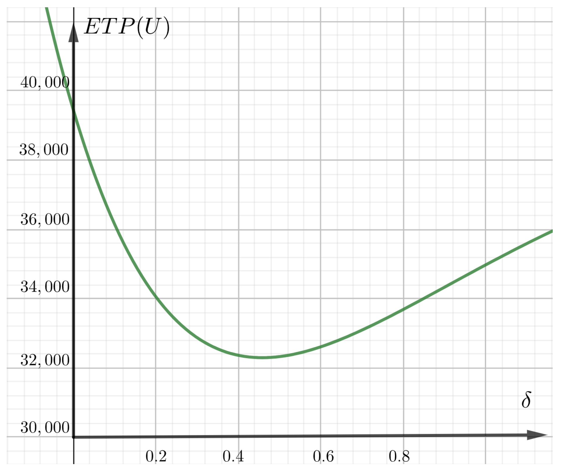
In this case of study, we consider the fractional model with short holding cost memory, i.e., δ = 1 and 0 < α 1 ; see Table 4. In this context, we observe that when we allow the integral memory index (0 < δ < 1) and the absence of the differential memory index, the critical value of the memory index is approximately 0.5, which is the lowest expected total profit. Similar to the previous model, at δ = 0.1 , the inventory reaches its peak E T P ( U ) of 39,329.03 when α = 0.1 . Then, it progressively decreases until α = 0.5 , at which point the inventory starts to recover. The projected total profit starts climbing again until the memory-less system. On the other hand, when the value of δ declines, the optimal ordering interval increases and eventually reaches a value that is not feasible in real-world scenarios. For this reason, we take the case where β = 1 , and we take the optimal value of the time cycle T 1 , 1 1 = 0.22 ; then we investigate E T P with respect to α (Figure 5).
Based on Figure 5, we employ the same interpretation as in the prior case where T is held constant.

6.4. Fractional Model with Long Memory IL and Holding Cost

The issue gets trickier for arbitrary values of α and δ . However, the problem can be solved numerically for specific values of α and δ . Here, in our discussion, we take α = 0.5 and δ = 0.5 .
We offer the optimal ETP(U) considering both memory effects simultaneously. We obtain the results shown in Table 5. We take, for example, the case where β = 1 ; the optimal ETP(U) equals 32,985.33 ZAR/year. Compared with the results shown in Table 4 (i.e., Table 5), these values came in between E T P 1 , 0.2 1 and E T P 1 , 0.1 1 (i.e., E T P 0.2 , 1 1 and E T P 0.1 , 1 1 ); therefore, the system was affected by long memory. In the long memory effect, businesses take a long time (5 years) to reach the maximum compared with the low memory effect or memory-less system. For the other case ( β = 0.9 , ), we obtain the same interpretation as in the previous case.

6.5. Sensitive Analysis

Purchasing cost and feeding cost are significant parameters that have a big influence on the overall total profit. The value of these two parameters is related to the weight of the items at the moment of purchase, which makes the purchasing moment significant.
In the following equation, we can determine the appropriate weight to obtain the optimal overall total profit, as follows:
f ( t ) = p · y · w t + c y t t 1 w x d x = p · y · A 1 + b · e λ · t + c · y · t t 1 w x d x , f ( t ) = p · y · A 1 + b · e λ · t + c · y · A λ ln b + e λ · t 1 ln b + e λ · t ,
To find the optimal weight, we solve the equation d f ( t ) d t = 0 , as follows:
d f ( t ) d t = y · A · b ( λ · p + c ) · e λ · t + c 1 + b · e λ · t 2 = 0 ,
Therefore,
e λ · t = c b ( λ · p + c ) .

6.5.1. Case I:

If c > λ · p :
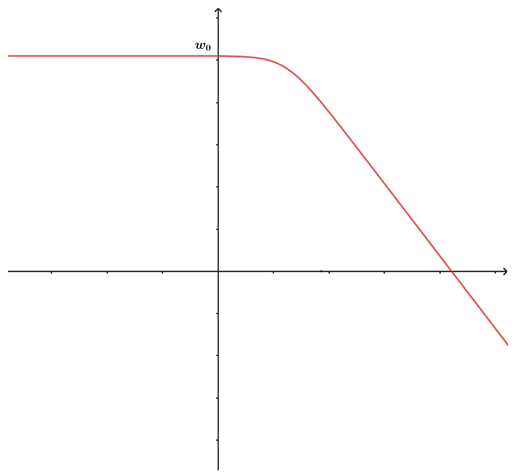
Figure 6 give the evolution of the function f in the case where c > λ · p . In this case, we can demonstrate d f ( t ) d t 0 ; therefore, f is a decreased function, so the closer the chicken’s weight is to w 1 , the better is the overall total profit.

6.5.2. Case II:

If c < λ · p and w t s < w t 1 , where
t s = 1 λ · ln c b ( λ · p + c ) .
  • Following Figure 7, if f ( t 1 ) f ( 0 ) , the closer the chicken’s weight is to w 1 , the better is the overall total profit.
  • If f ( t 1 ) f ( 0 ) , in this case, the smaller the weight of the chicken, the better the overall total profit.

6.6. Discussion

In our model, we handle two different memory effects, one effect in the inventory model level and the other effect the holding cost, and we reveal the existence of memory effects on inventory management, ordering interval, and ETP(U) in terms of fractional derivatives and integration. Based on the results in Table 3, Table 4 and Table 5, the business began with a sound policy and reached the highest ETP(U). In subsequent years, some poor policies were chosen, which led to a reduction in profit by decreasing ETP(U). This loss of profit is maximum at α = 0.6 (i.e., β = 0.5 ). The business again started recovery by choosing better policies for α = 0.6 (i.e., β = 0.5 ) as ETP(U) was increasing. Consequently, the company must reconsider its new policy or revert to the old policy to achieve better profit.
The selection of the weight for purchasing chickens depends on the feeding cost, the purchasing cost, and the rate of growth.
Based on the data illustrated, in Figure 8, we have the following: (a) every parameter—aside from demand—has an adverse effect on the anticipated total profit per unit time, (b) the demand rate has the greatest impact on ETP(U), and (c) the alterations in the setup and holding costs have the second most significant influence on the anticipated overall profit, but with a less dramatic effect compared with the demand rate.

7. Conclusions

In inventory modeling, it is important to consider the impact of memory or past experience effects. These effects are based on the idea that entrepreneurs may recall the historical changes in exogenous and endogenous variables that define economic operation. Practically speaking, the fractional order inventory model is more advantageous in real systems than the classical inventory model. In this paper, we introduced a fractional economic order quantity (FEGQ) model for growing products to account for the memory effect. Three essential cases of study are examined: (a) short-term memory of holding costs, (b) short-term memory of inventory levels, and (c) long-term memory of inventory levels and holding costs.
We used the FEGQ model to determine the optimal length of the consumption period and the maximum total profit expected in the context of the chicken breed. The experiment was based on real-life data. The results obtained were compared with those obtained by conventional EOQ models. The proposed model has improved ETP(U) by 13.92 % .
Concerning the management side, the provided numerical data indicate that the firm began with a favorable policy. In the following years, several misguided practices were implemented that resulted in a decrease in profitability. The process of healing commenced once more by selecting more effective strategies. In addition, we conducted a sensitivity analysis and discussed how to select the appropriate initial weights to achieve optimal overall total profit. In this sense, we examined how variations in the main parameters of the model can affect ETP(U). The initial weight is strongly affected by the feeding cost, the purchasing cost, and the growth rate. This work can help business policy makers to include the level of past experience in the marketing system.
While it is true that the proposed fractional model can significantly improve the ETP(U) benefit, the optimal cycle time, in the case of long-memory modeling, it requires a long period of time to reach the optimal cycle time. In addition, as the Newton–Raphson numerical method has a high order of error, our method may lose some of its accuracy.
In the future, we intend to use heuristic methods to determine optimal splitting orders and improve decision quality from an initial population produced by Raphson–Newton.

Author Contributions

Conceptualization, A.O.; methodology, K.E.M.; validation, A.-M.P.; investigation, A.O. and A.-M.P.; writing—review and editing, F.B. and A.-M.P.; visualization, F.B.; supervision, K.E.M.; All authors have read and agreed to the published version of the manuscript.

Funding

The APC was funded by Dunărea de Jos University of Galaţi, under the project RF2488/31.05.2024.

Data Availability Statement

Dataset available on request from the authors.

Acknowledgments

The authors thank the anonymous referees for their valuable comments and suggestions in the initial version of our article.

Conflicts of Interest

The authors declare no conflicts of interest.

References

  1. Harris, F.W. How Many Parts to Make at Once. Factory Mag. Manag. 1913, 10, 135–136, 152. [Google Scholar] [CrossRef]
  2. Wilson, R.H. A Scientific Routine for Stock Control; Harvard University: Cambridge, MA, USA, 1934. [Google Scholar]
  3. Podlubny, I. Fractional Differential Equations: An Introduction to Fractional Derivatives, Fractional Differential Equations, to Methods of Their Solution and Some of Their Applications; Elsevier: Amsterdam, The Netherlands, 1998. [Google Scholar]
  4. Tenreiro Machado, J.A. Fractional Derivatives and Their Applications. In Proceedings of the Sixth EUROMECH Nonlinear Dynamics Conference, Saint Petersburg, Russia, 30 June–4 July 2008; pp. 1–27. [Google Scholar]
  5. Baleanu, D.; Güvenç, Z.B.; Machado, J.T. New Trends in Nanotechnology and Fractional Calculus Applications; Springer: New York, NY, USA, 2010; Volume 10, pp. 978–990. [Google Scholar]
  6. Machado, J.T.; Mata, M.E. Pseudo Phase Plane and Fractional Calculus Modeling of Western Global Economic Downturn. Commun. Nonlinear Sci. Numer. Simul. 2015, 22, 396–406. [Google Scholar] [CrossRef]
  7. Agila, A.; Baleanu, D.; Eid, R.; Irfanoglu, B. Applications of the Extended Fractional Euler-Lagrange Equations Model to Freely Oscillating Dynamical Systems. Rom. J. Phys. 2016, 61, 350–359. [Google Scholar]
  8. Das, A.K.; Roy, T.K. Fractional Order EGQ Model with Linear Trend of Time-Dependent Demand. Int. J. Intell. Syst. Appl. 2015, 3, 44–53. [Google Scholar]
  9. Das, A.K.; Roy, T.K. Fractional Order Generalized EPQ Model. Int. J. Comput. Appl. Math. 2017, 12, 525–536. [Google Scholar]
  10. Pakhira, R.; Ghosh, U.; Sarkar, S. Study of Memory Effects in an Inventory Model Using Fractional Calculus. Appl. Math. Sci. 2018, 12, 797–824. [Google Scholar] [CrossRef]
  11. Pakhira, R.; Ghosh, U.; Sarkar, S. Application of Memory Effects in an Inventory Model with Linear Demand and No Shortage. Int. J. Res. Advent Technol. 2018, 6, 8. [Google Scholar]
  12. Rahaman, M.; Mondal, S.P.; Shaikh, A.A.; Ahmadian, A.; Senu, N.; Salahshour, S. Arbitrary-Order Economic Production Quantity Model with and without Deterioration: Generalized Point of View. Adv. Differ. Equ. 2020, 2020, 16. [Google Scholar] [CrossRef]
  13. Das, A.K.; Roy, T.K.; Jana, D.K. Fractional order generalized EGQ model with demand-dependent unit purchasing cost under space constraints. In Recent Advances in Intelligent Information Systems and Applied Mathematics; Springer: New York, NY, USA, 2020; pp. 1–17. [Google Scholar]
  14. Rahaman, M.; Mondal, S.P.; Alam, S. An Estimation of Effects of Memory and Learning Experience on the EGQ Model with Price Dependent Demand. Rairo-Oper. Res. 2021, 55, 2991–3020. [Google Scholar] [CrossRef]
  15. Rahaman, M.; Mondal, S.P.; Chatterjee, B.; Alam, S.; Shaikh, A.A. Generalization of Classical Fuzzy Economic Order Quantity Model Based on Memory Dependency via Fuzzy Fractional Differential Equation Approach. J. Uncert. Sys. 2022, 15, 2250003. [Google Scholar] [CrossRef]
  16. Rezaei, J. Economic Order Quantity for Growing Items. Int. J. Prod. Econ. 2014, 155, 109–113. [Google Scholar] [CrossRef]
  17. Msomi, A.M.; Bansilal, S. Analysis of Students’ Errors and Misconceptions in Solving Linear Ordinary Differential Equations Using the Method of Laplace Transform. Int. Electron. J. Math. Educ. 2022, 17, em0670. [Google Scholar] [CrossRef]
  18. West, B.J. Exact Solution to Fractional Logistic Equation. Phys. A Stat. Mech. Its Appl. 2015, 429, 103–108. [Google Scholar] [CrossRef]
  19. Area, I.; Losada, J.; Nieto, J.J. A Note on the Fractional Logistic Equation. Phys. A Stat. Mech. Its Appl. 2016, 444, 182–187. [Google Scholar] [CrossRef]
  20. Bhalekar, S.; Daftardar-Gejji, V. Solving Fractional-Order Logistic Equation Using a New Iterative Method. Int. J. Differ. Equ. 2012, 2012, 1–12. [Google Scholar] [CrossRef]
  21. Momani, S.; Qaralleh, R. Numerical Approximations and Padé Approximants for a Fractional Population Growth Model. Appl. Math. Model. 2007, 31, 1907–1914. [Google Scholar] [CrossRef]
  22. Sumiati, I.; Bon, S.A. Adomian Decomposition Method and the New Integral Transform. In Proceedings of the 2nd African International Conference on Industrial Engineering and Operations Management, Harare, Zimbabwe, 7–10 December 2020; pp. 1882–1887. [Google Scholar]
  23. Ouhmid, A.; Belhabib, F.; Elkari, B.; El Moutaouakil, K.; Ourabah, L.; Benslimane, M.; El Mekkaoui, J. Economic Growing Quantity: Broiler Chicken in Morocco. Stat. Optim. Inf. Comput. 2024, 12, 817–828. [Google Scholar] [CrossRef]
  24. El Moutaouakil, K.; Bouhanch, Z.; Ahourag, A.; Aberqi, A.; Karite, T. OPT-FRAC-CHN: Optimal Fractional Continuous Hopfield Network. Symmetry 2024, 16, 921. [Google Scholar] [CrossRef]
  25. El Moutaouakil, K.; El Ouissari, A.; Palade, V.; Charroud, A.; Olaru, A.; Baïzri, H.; Chellak, S.; Cheggour, M. Multi-Objective Optimization for Controlling the Dynamics of the Diabetic Population. Mathematics 2023, 11, 2957. [Google Scholar] [CrossRef]
  26. Sebatjane, M.; Adetunji, O. Economic Order Quantity Model for Growing Items with Imperfect Quality. Oper. Res. Perspect. 2019, 6, 100088. [Google Scholar] [CrossRef]
  27. Gdawiec, K.; Kotarski, W.; Lisowska, A. Newton’s Method with Fractional Derivatives and Various Iteration Processes via Visual Analysis. Numer. Algor. 2021, 86, 953–1010. [Google Scholar] [CrossRef]
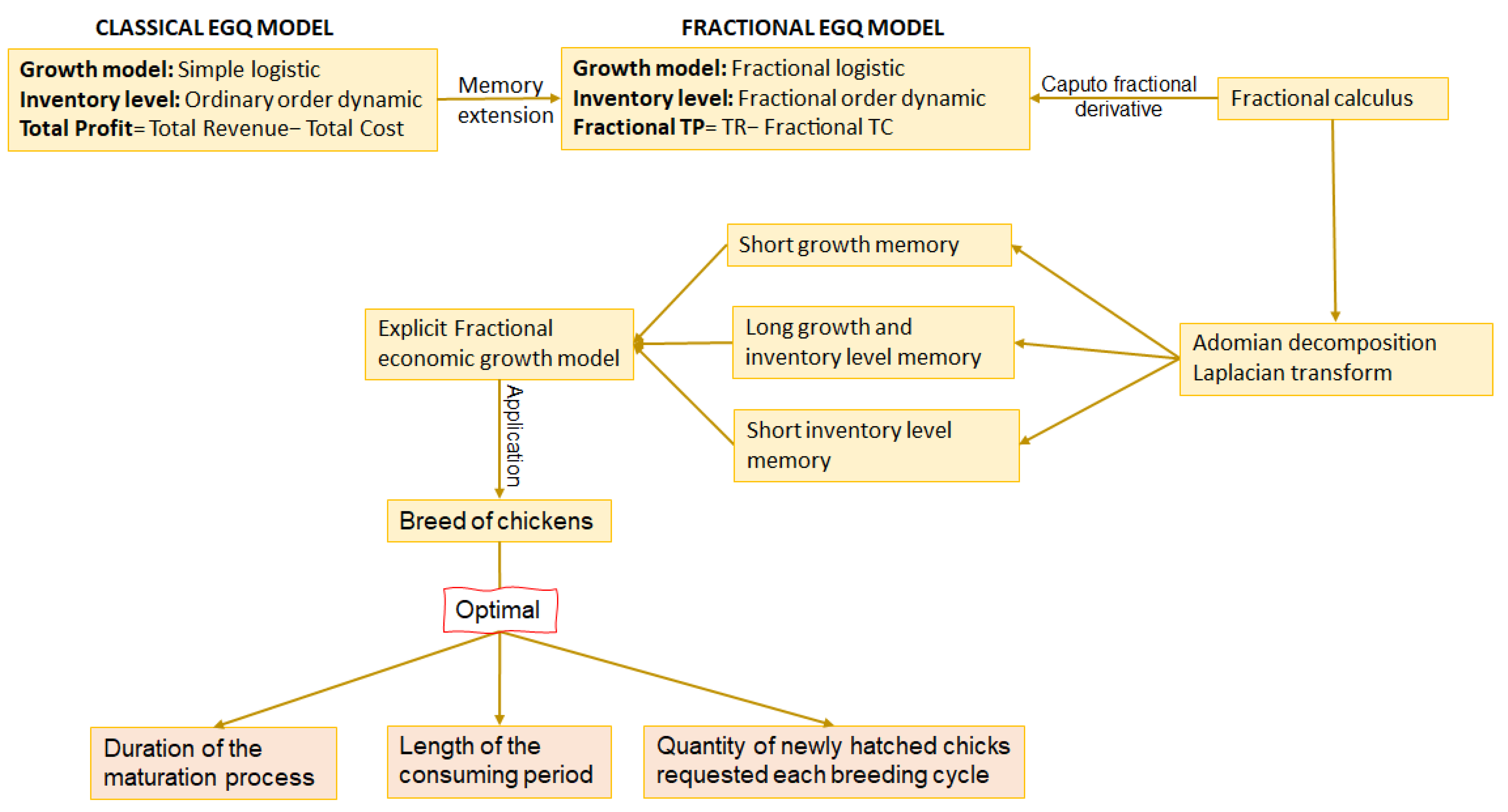
Figure 1. Methodology adopted in this paper to build the FEGQ model.
Symmetry 16 01057 g001
Figure 2. The evolution of the weight of newborn chick per time.
Symmetry 16 01057 g002
Figure 3. Evolution of inventory system over time.
Symmetry 16 01057 g003
Figure 4. ETP(U) and the optimal cycle duration in the case α > 0 and δ = β = 1 .
Symmetry 16 01057 g004
Figure 5. ETP(U) in the function of δ with T fixed and β = α = 1 .
Symmetry 16 01057 g005
Figure 6. The evolution of the function f in the case where c > λ · p .
Symmetry 16 01057 g006
Figure 7. The evolution of the function f in the case where c < λ · p .
Symmetry 16 01057 g007
Figure 8. ETP(U) variation brought on by parameter changes.
Symmetry 16 01057 g008
Table 1. Parameters and decision variables of the EGQ model.
Parameters
w 0 Weight of newly hatched chicks (g)
w 1 Desired mass (g)
NItem’s yearly demand rate (g/year)
ACarrying capacity (g)
nIntegration constant of the growth function
λ growth rate
Decision Parameter
yQuantity of newly hatched chicks requested at each breeding cycle
TTime span of the consumption phase (in years)
Cost components
p Price per unit (ZAR/g)
sPrice of selling an individual item (ZAR/g)
H The expense associated with storing a single unit of an item throughout the period of consumption (ZAR /g/year)
h Cost of maintaining a single unit item during the breeding period (ZAR /items)
KCapital of setting required for each growth cycle (ZAR)
qVaccination expenses
c Feeding expenses (ZAR/g)
Time period
t 1 Duration of the maturation process (in years)
TLength of the consuming period (in years)
Table 2. ETP(U) and the optimal cycle duration in the case α = 1 and δ = 1 .
α β
10.950.90.850.80
E T P T t 1 ¯ E T P T t 1 E T P T t 1 E T P T t 1 E T P T t 1
134,973.460.2230.087835,820.390.2230.07236,603.060.2230.05837,443.060.2230.04538,139.060.2230.034
Table 3. ETP(U) and the optimal cycle duration in the case α > 0 and δ = 1 .
α β
10.950.90.850.80
E T P T t 1 ¯ E T P T t 1 E T P T t 1 E T P T t 1 E T P T t 1
134,973.460.2230.087835,820.390.2230.07236,603.060.2230.05837,443.060.2230.04538,139.060.2230.034
0.934,597.220.2210.087835,408.000.2210.07236,155.650.2200.05836,960.070.2200.04537,623.150.2200.034
0.834,286.140.2210.087835,054.910.2210.07235,761.410.2200.05836,523.280.2200.04537,146.260.2190.034
0.734,076.660.2250.087834,799.900.2240.07235,460.630.2230.05836,174.420.2230.04536,751.310.2230.034
0.634,019.850.2340.087834,696.630.2330.07235,310.270.2320.05835,973.870.2310.04536,501.980.2310.034
0.534,184.180.2510.087834,819.520.2500.07235,390.690.2490.05836,008.580.2490.04536,491.830.2500.034
0.434,665.080.2820.087835,273.150.2820.07235,816.350.2820.05836,404.170.2840.04536,858.040.2860.034
0.335,600.190.3470.087836,209.120.340.07236,753.910.3520.05837,344.490.3570.04537,802.340.3640.034
0.237,202.780.5120.087837,859.940.520.07238,456.910.5370.05839,104.440.5560.04539,621.400.5780.034
0.139,842.331.310.087840,609.641.390.07241,318.281.490.05842,086.451.60.04542,719.151.720.034
Table 4. ETP(U) and the optimal cycle duration in the case α = 1 and δ > 0 .
α β
10.950.90.850.80
E T P T t 1 E T P T t 1 E T P T t 1 E T P T t 1 E T P T t 1
0.934,329.610.2200.087835,188.550.2200.07235,959.210.2200.05836,799.210.2200.04537,495.210.2200.034
0.833,687.840.2190.087834,546.780.2190.07235,317.440.2190.05836,157.440.2190.04536,853.440.2190.034
0.733,092.950.2240.087833,951.880.2240.07234,722.550.2240.05835,562.550.2240.04536,258.550.2240.034
0.632,621.550.2360.087833,480.480.2360.07234,251.150.2360.05835,091.150.2360.04535,787.150.2360.034
0.532,400.080.2600.087833,259.010.2600.07234,029.680.2600.05834,869.680.2600.04535,565.680.2600.034
0.432,629.160.3100.087833,488.090.3100.07234,258.760.3100.05835,098.760.3100.04535,794.760.3100.034
0.333,608.250.4200.087834,467.190.4200.07235,237.850.4200.05836,077.850.4200.04536,773.850.4200.034
0.235,729.970.7320.087836,588.910.7320.07237,359.570.7320.05838,199.570.7320.04538,895.570.7320.034
0.139,329.032.3970.087840,187.962.3970.07240,958.632.3970.05841,798.632.3970.04542,494.632.3970.034
Table 5. ETP(U) and the optimal cycle duration in the case α = 0.5 and δ = 0.5 .
α β
10.950.90.850.80
α = 0.5 and δ = 0.5 E T P T t 1 ¯ E T P T t 1 E T P T t 1 E T P T t 1 E T P T t 1
32,985.335.030.087833,826.93116.130.07234,597.3120.20.05835,437.1121.30.04536,132.9127.80.034
Disclaimer/Publisher’s Note: The statements, opinions and data contained in all publications are solely those of the individual author(s) and contributor(s) and not of MDPI and/or the editor(s). MDPI and/or the editor(s) disclaim responsibility for any injury to people or property resulting from any ideas, methods, instructions or products referred to in the content.