UAV Tracking via Saliency-Aware and Spatial–Temporal Regularization Correlation Filter Learning

Abstract

Due to their great balance between excellent performance and high efficiency, discriminative correlation filter (DCF) tracking methods for unmanned aerial vehicles (UAVs) have gained much attention. Due to these correlations being capable of being efficiently computed in a Fourier domain by discrete Fourier transform (DFT), the DFT of an image has symmetry in the Fourier domain. However, DCF tracking methods easily generate unwanted boundary effects where the tracking object suffers from challenging situations, such as deformation, fast motion and occlusion. To tackle the above issue, this work proposes a novel saliency-aware and spatial–temporal regularized correlation filter (SSTCF) model for visual object tracking. First, the introduced spatial–temporal regularization helps build a more robust correlation filter (CF) and improve the temporal continuity and consistency of the model to effectively lower boundary effects and enhance tracking performance. In addition, the relevant objective function can be optimized into three closed-form subproblems which can be addressed by using the alternating direction method of multipliers (ADMM) competently. Furthermore, utilizing a saliency detection method to acquire a saliency-aware weight enables the tracker to adjust to variations in appearance and mitigate disturbances from the surroundings environment. Finally, we conducted numerous experiments based on three different benchmarks, and the results showed that our proposed model had better performance and higher efficiency compared to the most advanced trackers. For example, the distance precision (DP) score was 0.883, and the area under the curve (AUC) score was 0.676 on the OTB2015 dataset.

1. Introduction

Visual object tracking [1,2,3,4] plays a momentous role in the domain of computer vision, which is widely used in various applications, such as autonomous driving, robotics, telemedicine and so on. Applying tracking methods through airborne unmanned aerial vehicles (UAVs) extensively facilitates UAV-based applications, such as proof of autonomous aerial manipulation operations [2], collision avoidance and automatic transmission line detection. The aim of object tracking is achieved by modeling the object according to the initial state of the given object, then evaluating the status of the object in a subsequent video sequence, and finally giving location and scale information. As one of the critical techniques in computer vision, visual object tracking is of great significance in target detection, recognition, segmentation, image analysis and understanding [5]. With the rapid development of artificial intelligence, many object tracking methods [6,7] have been proposed, and the research on object tracking technology has made remarkable achievements. However, due to the interference of various factors that often occur during object tracking, such as fast motion, background clutter and deformation, there is still a great challenge in building a robust visual tracking system.

Recently, a visual tracking algorithm based on a discriminant correlation filter (CF) not only ensures accuracy, but also has efficient real-time performance, and has gained much attention by many researchers. Traditional correlation filter methods [8,9,10] use the properties of a cyclic matrix to obtain training samples and solve the correlation filtering model in z frequency domain by using fast Fourier transform (FFT). The DCF model achieves real-time tracking performance and, finally, learns a classifier with strong discrimination to differentiate between the target and the background. For instance, MOSSE [8] first introduced the correlation filter into tracking, achieving excellent performance with a speed of 600 frames per second. The kernel function and multi-channel HOG features are incorporated into the correlation filter framework with a kernel correlation filter (KCF), which achieves a robust performance with a high speed, effective tracking under motion blur, illumination variation and color change situation.

The standard DCF method can greatly improve computational efficiency [11]. However, the training samples based on the kernel correlation filter are obtained by cyclic shifting of the central target. This process generates many unrealistic samples which result in numerous undesired boundary effects [12]. The induced boundary effect limits the standard DCF model in two primary aspects. Firstly, the unreal training samples weaken the discriminatory power of the learned model and cause it to lose important information. Secondly, non-central points within the detection area are ignored during calculation due to the strong influence from periodic repetitions of the detection sample. To deal with the above border effects of the CF tracker, many excellent trackers have been designed that have achieved a better performance and reached a good tracking speed [13,14,15,16,17,18,19,20]. For instance, the SRDCF tracker [13] tackles this issue by introducing a spatial regularization component, enabling the correlation filter to learn over a larger image region, thereby creating a more discriminating appearance model. Nevertheless, the foremost disadvantage of the SRDCF tracker is the high cost of computation due to its regularization operation, so it cannot be used for real-time tasks. The BACF [14] tracker utilizes genuine background blocks and target blocks to enhance more differentiated trackers, while utilizing an online adaptive strategy to renew the tracker model. The proposed long-term RGB-D [21] tracker solves the limitation of modeling appearance changes associated with out-of-plane rotation via an Object Tracking by Reconstruction (OTR) approach. A target-dependent feature network [22] incorporates cross-image feature associations into multiple layers. The recently developed ASRCF method [15] adds an adaptive spatial component to the objective function and optimizes function using the ADMM algorithm [16] for learning reliable filter coefficients. A spatial–temporal regularized CF [17] was proposed via introducing temporal regularization into the SRDCF method with a single sample, and it obtained more training samples and also assisted in creating a sounder layout model for object tracking. The proposed autotracker method [18] uses an automatic spatial–temporal regularization framework for high-performance UAV tracking, using the partial response and global variation for restricting and controlling correlation filter learning, and the tracking speed reaches 60 fps with an evaluation of CPU. As convolutional neural networks (CNNs) develop rapidly, many trackers are being proposed using deep networks to extract depth features. These trackers significantly enhance tracking accuracy and robustness but increase the speed of calculation while reducing the tracking speed. Examples are Deep SRDCF [23], C-COT [24], RPCF [25], CFNet [26] and DeepSTRCF [17].

In this paper, we put forward a novel saliency-aware and spatial–temporal regularized correlation filter (SSTCF) for visual object tracking. The main contributions can be expressed as the following:

• We integrated a spatial–temporal regularization term into the formulation of multiple training samples to combine DCF learning and model updating, which was conducive to tracking accuracy and robustness, and it could adapt to changes in the appearance of different objects at different times.
• The saliency detection method is employed to acquire a saliency-aware weight so that the tracker can adapt to appearance changes and suppress background interference.
• Unlike the SRDCF, which produced high complexity by using multiple training image processing methods, the ADMM algorithm can be utilized to effectively optimize the SSTCF model, which the three subproblems have the analytic solutions.
• We evaluated the SSTCF tracker on two classic tracking benchmarks and the latest long-term UAV tracking datasets, which were the OTB2015 dataset [27], the VOT2018 dataset [28], and the LASOT dataset [29]. Experimental results display that the SSTCF tracker has higher accuracy and real-time performance than many existing methods.

2. Related CF-Based Models

2.1. Standard DCF

The Kernel Correlation filter [10] method transforms the solution of the correlation filter into the ridge regression problem, which is a regularized least squares method with high efficiency and a closed solution. It utilizes the properties of cyclic matrices for intensive sampling. The operation of cyclic shift greatly improved the performance and efficiency of the CF-trackers. In spatial domain, the objective function formulation of the standard DCF model is as shown below,

$$E(h)={\displaystyle \frac{1}{2}}{‖{\displaystyle \sum _{k=1}^K{x}_k\ast h_k}-y‖}_2^2+{\displaystyle \frac{\lambda }{2}}{\displaystyle \sum _{k=1}^K{‖h_k‖}_2^2}$$

(1)

where $x_k\in {ℝ}^{D\times 1}$ indicates the $k$-th channel of the vectorized image, $K$ is the total number of channels, and $h_k\in {ℝ}^{D\times 1}$ denotes the $k$-th channel of the vectorized filter. The vector $y\in {ℝ}^{D\times 1}$ is a reply to expectations and generally utilizes a Gaussian shape of the ground truth in general. The symbol $\ast$ means the spatial correlation operator, and $\lambda$ is a regularization parameter.

The standard DCF model trains discriminative CF trackers using a set of training samples, adopting a circular shift operator on the tracked object to obtain negative training samples. However, due to the cyclic shift operation, only the center sample is accurately positive. When the objective function of the DCF model is solved in the frequency domain, because of the cyclic shift of the samples, the boundary position is prone to periodic repetition. A flaw hidden in the correlation filtering model is the boundary effect, and it is easy to overfit, which results in poor robustness and discrimination ability of the classifier and decreases the performance of the tracker. To address this problem, several trackers have been proposed. For instance, the SRDCF [13] and BACF [14] trackers introduced spatial constraints and a diagonal binary matrix, respectively, into the objective functions to reduce the impact of boundary effects.

2.2. Spatially Regularized Discriminative Correlation Filters (SRDCF)

The SRDCF [13] algorithm was introduced based on the standard DCF model, converting the spatial regularization term into an objective function. The introduced Tikhonov regularization and spatial weights aim to penalize the filter coefficients according to their spatial locations. The related objective function is

$$E(h)={\displaystyle \frac{1}{2}}{‖{\displaystyle \sum _{k=1}^K{x}_k\ast h_k}-\mathrm{y}‖}_2^2+{\displaystyle \frac{\lambda }{2}}{\displaystyle \sum _{k=1}^K{‖w\odot h_k‖}_2^2}$$

(2)

where $w$ is a negative Gaussian-shaped spatial weight vector. The authors found that the image features near the edge of the target are inclined to be less reliable than the features near the center of the target, so it is possible to shift the regularization weight smoothly from the target area to the background area. This also increases the sparsity of $w$ in the Fourier domain. Although SRDCFs can productively inhibit the boundary effect, the high amount of calculation is the main problem of this method. The spatial regularization term cannot well utilize the circular CF matrix, and the extensive system of linear equations and the Gauss–Seidel method are very time-consuming, leading to many calculations.

2.3. Background-Aware Correlation Filters (BACF)

As we know, Equation (1) can be equivalently expressed as an objective equation of ridge regression. Based on DCFs, the authors of [14] proposed background-aware correlation filters (BACFs). Their objective function can be expressed as follows:

$$E(h)={\displaystyle \frac{1}{2}}{\displaystyle \sum _{j=1}^T{‖{\displaystyle \sum _{k=1}^K{h_k}^{{\rm T}}}P{x}_k\left[\Delta {\mathit{\tau }}_j\right]-y\left(\mathrm{j}\right)‖}_2^2}+{\displaystyle \frac{\lambda }{2}}{\displaystyle \sum _{k=1}^K{‖h_k‖}_2^2}$$

(3)

where $\left[\Delta {\mathit{\tau }}_j\right]$ is the cyclic shift operation, and $x_k\left[\Delta {\mathit{\tau }}_j\right]$ indicates the discrete cyclic shift of step $j$, operated on the features $x_k$ of channel $k$. $P$ is a binary mask matrix clipping a $T\times D$ matrix from the object feature $x_k$, and $T$ ≫ $D$, where $T$ is the length of $x$, $x_k\in {ℝ}^T$, $y\in {ℝ}^T$, and $h\in {ℝ}^D$. The symbol ${ }^{{\rm T}}$ is the conjugate transpose.

The BACF method uses a binary mask matrix to search for samples and uses dense sampling to obtain true positive and negative samples, thereby reducing the effect of the cyclic shift on the boundary effect. In addition, the BACF method optimizes the objective function by efficiently using the ADMM algorithm, reducing the computational burden.

3. Proposed Method

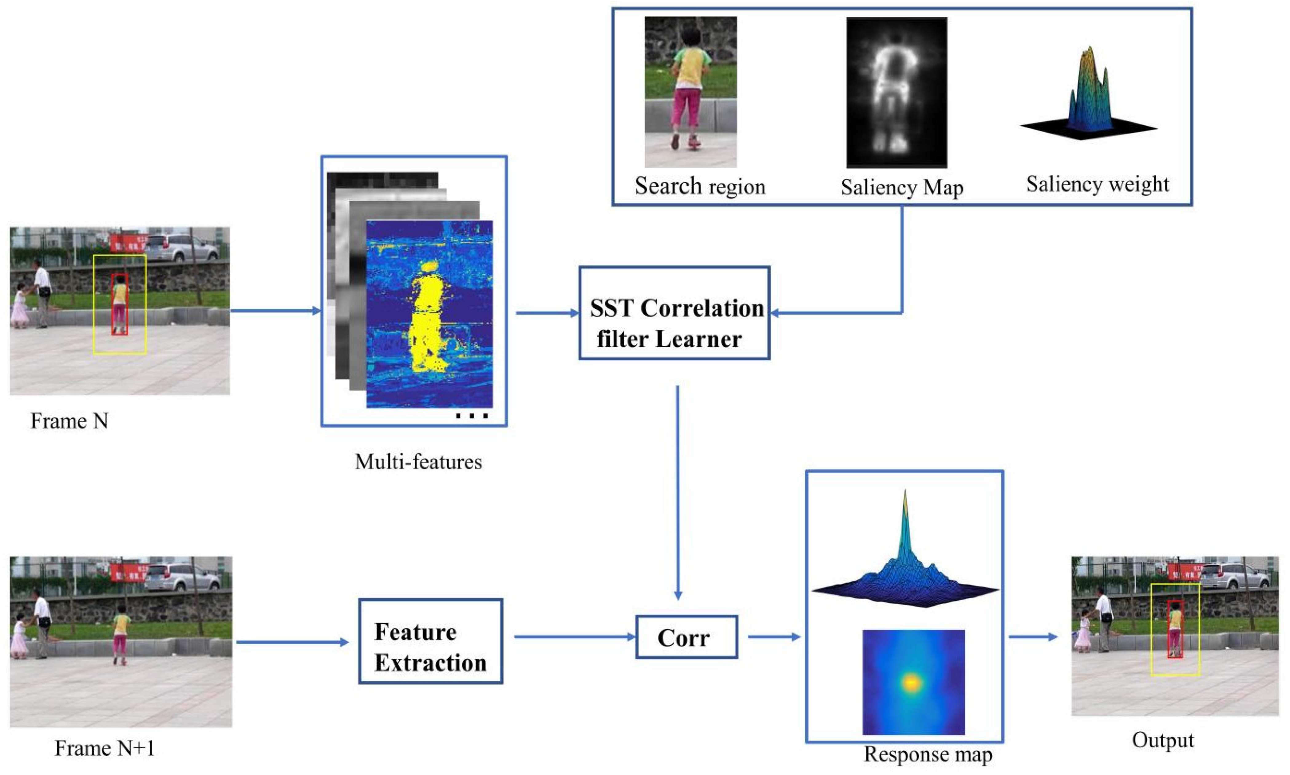
3.1. The Overall Framework

Figure 1 illustrates the overall framework of our proposed SSTCF method. We take the Girl2 sequence as an example in this section. We aimed to train a saliency-aware and spatial–temporal regularized correlation filter in frame N. For the feature extraction module, we used multiple features, including shallow HOG features, color names, and deep CNN features, which assisted in constructing a more robust apparent model. Then, the object function based on spatial regularization and a time-resolved term was transformed into the frequency domain, and the ADMM algorithm was utilized to efficiently solve the subproblem. Meanwhile, we replaced the spatial weight with saliency-aware weight to efficiently adapt to significant changes in the shape of the tracked object and inhibit irrelevant background noise in the correlation filter.

For the SSTCF method, we applied a saliency-aware weight, the value of which was updated in each frame to adapt to appearance and time changes. As shown in the Girl2 sequence image in Figure 1, the saliency perception suppressed background interference and assigned a greater penalty to the relevant pixels. Additionally, the response map reflects our SSTCF model and indicates the peak responses.

3.2. Saliency-Aware and Spatial-Temporal Regularized Model

3.2.1. Objective Function of Spatial-Temporal Regularized Model

In order to lower the effect of performance tracking on unnecessary boundary effects, we added spatial and temporal regularization terms to the objective function. The STRCF [17] and BACF [14] methods gave us inspiration. First, the concept of spatial regularization was incorporated into the construction of the objective function, which is beneficial for DCF learning and model updating. Second, to improve the temporal continuity and consistency of the model, a temporal-aware term was introduced into the objective function to compensate for the large variation in the two-frame correlation filter. Thus, we took ${‖P^{{\rm T}}{h}_k-P^{{\rm T}}{h}_k^{v-1}‖}_2^2$ as the temporal-aware term, with which the temporal constraint was able to improve the temporal continuity and consistency of the model, where $h_k^{v-1}$ represents a learned filter for the last frame. So, our objective function can be expressed as follows:

$$E(h,w)={\displaystyle \frac{1}{2}}{\displaystyle \sum _{j=1}^T{‖{\displaystyle \sum _{k=1}^K(P^{{\rm T}}{h}_k)\ast }{x}_k\left[\Delta {\mathit{\tau }}_j\right]-y\left(\mathrm{j}\right)‖}_2^2}+{\displaystyle \frac{{\lambda }_1}{2}}{\displaystyle \sum _{k=1}^K{‖w\odot h_k‖}_2^2} +{\displaystyle \frac{\beta }{2}}{‖P^{{\rm T}}{h}_k-P^{{\rm T}}{h}_k^{v-1}‖}_2^2$$

(4)

where $x_k\in {ℝ}^T$, $y\in {ℝ}^T$, $h\in {ℝ}^D$, and $P\in {ℝ}^{T\times T}$ represent a diagonal binary matrix. In this work, the correlation operator was used directly in the filter template, and the correlation operator was evaluated according to the target features. ${\lambda }_1$ is a spatial regularization parameter for the second and third terms. The parameter $w$ indicates the spatial weight. A priori information is introduced to the spatial weight $w$ to effectively avoid model degradation. $\beta$ is a regularization parameter of temporal awareness, and ${ }^{{\rm T}}$ is the conjugate transposition operation.

3.2.2. Algorithm Optimization

It was observed that Equation (5) can be addressed iteratively to acquire the optimal solution through the ADMM algorithm because it is a convex function. Inspired by the previous correlation filter tracking method, the correlation filter can be trained productively in the frequency domain. Therefore, we converted the objective function to the frequency domain by utilizing Parseval’s theorem, and we introduced an auxiliary variable $\widehat{g}$ for the solution. The equality-constrained optimization form in the frequency domain is as follows:

$$\begin{array}{l}E(h,\widehat{g,}w)={\displaystyle \frac{1}{2T}}{‖\widehat{X}\widehat{g}-\widehat{y}‖}_2^2+{\displaystyle \frac{{\lambda }_1}{2}}{‖w\odot h‖}_2^2 +{\displaystyle \frac{\beta }{2}}{‖\widehat{g}-{\widehat{g}}_{v-1}‖}_2^2\hfill \\ s.t. \widehat{g}=\sqrt{T}F{P}^{{\rm T}}h\hfill \end{array}$$

(5)

where $\widehat{X}=\left[diag{(\widehat{x_1})}^{{\rm T}},\dots ,diag{(\widehat{x_K})}^{{\rm T}}\right]\in {ℝ}^{T\times KT}$ and $h={\left[h_1^{{\rm T}},\dots ,h_K^{{\rm T}}\right]}^{{\rm T}}\in {ℝ}^{KT\times 1}$, giving a cascade of correlation filter vectorization with $K$ channels, and $\widehat{g}={\left[{\widehat{g}}_1^{{\rm T}},\dots ,{\widehat{g}}_K^{{\rm T}}\right]}^{{\rm T}}\in {ℝ}^{KT\times 1}$. The symbol $\widehat{ }$ represents the discrete Fourier transform of the signal, and $F$ is the orthonormal $T\times T$ matrix of complex basis vectors to map any $T$ dimensional vectorized signal into the Fourier domain. For instance, $\widehat{a}=\sqrt{T}Fa$. ${\widehat{g}}_{v-1}=\sqrt{T}F{P}^{{\rm T}}{h}_{v-1}$ is an auxiliary variable, where $h_{v-1}$ is analogous to $h$.

This shows that the model in Equation (5) is convex, and the optimal solution can be obtained by iterating the ADMM. Thus, we first optimized Equation (5) using the augmented Lagrangian method (ALM), where the Lagrangian can be expressed as follows:

$$\begin{array}{ll}L(h,\widehat{g,}\widehat{\xi },w)& ={\displaystyle \frac{1}{2T}}{‖\widehat{X}\widehat{g}-\widehat{y}‖}_2^2+{\displaystyle \frac{{\lambda }_1}{2}}{‖w\odot h‖}_2^2 +{\displaystyle \frac{\beta }{2}}{‖\widehat{g}-{\widehat{g}}_{v-1}‖}_2^2\\ & +{\widehat{\xi }}^{{\rm T}}(\widehat{g}-\sqrt{T}F{P}^{{\rm T}}h)+{\displaystyle \frac{\mu }{2}}{‖\widehat{g}-\sqrt{T}F{P}^{{\rm T}}h‖}_2^2\end{array}$$

(6)

where $\widehat{\xi }={\left[{\widehat{\xi }}_1^{{\rm T}},\dots ,{\widehat{\xi }}_K^{{\rm T}}\right]}^{{\rm T}}$, a collection of the Lagrange multipliers, and $\mu$ is a penalty factor. We can use the ADMM algorithm to solve the subproblems $\widehat{g}$ and $h$ and update $\widehat{\xi }$.

• Subproblem $h$

If variables $\widehat{g}$ and $\widehat{\xi }$ are invariant in Equation (5), we can obtain the closed-form solution for variable $h$. Therefore, $h$ can be calculated as follows:

$$h=\underset{h}{\arg \min }\left\{{\displaystyle \frac{{\lambda }_1}{2}}{‖w\odot h‖}_2^2 +{\widehat{\xi }}^{{\rm T}}(\widehat{g}-\sqrt{T}F{P}^{{\rm T}}h)+{\displaystyle \frac{\mu }{2}}{‖\widehat{g}-\sqrt{T}F{P}^{{\rm T}}h‖}_2^2\right\}$$

(7)

Equation (5) can be formulated as follows:

$$C(h)={\displaystyle \frac{{\lambda }_1}{2}}{‖w\odot h‖}_2^2 +{\widehat{\xi }}^{{\rm T}}(\widehat{g}-\sqrt{T}F{P}^{{\rm T}}h)+{\displaystyle \frac{\mu }{2}}{‖\widehat{g}-\sqrt{T}F{P}^{{\rm T}}h‖}_2^2$$

(8)

where $W=diag(w)\in {ℝ}^{T\times T}$, $w\odot h=Wh$. Then, the partial derivative $C(h)$ is taken as follows:

$$\begin{array}{ll}{\displaystyle \frac{\partial C(h)}{\partial h}}& ={\displaystyle \frac{\partial }{\partial h}}({\displaystyle \frac{{\lambda }_1}{2}}{‖Wh‖}_2^2 +{\widehat{\xi }}^{{\rm T}}(\widehat{g}-\sqrt{T}F{P}^{{\rm T}}h)+{\displaystyle \frac{\mu }{2}}{‖\widehat{g}-\sqrt{T}F{\mathit{P}}^{{\rm T}}h‖}_2^2)\\ & = ({\lambda }_1{W}^{{\rm T}}W+ \mu T P{F}^{{\rm T}}F{P}^{{\rm T}}) h-\sqrt{T}{(\mathbf{F}{\mathit{P}}^{{\rm T}})}^{{\rm T}}\widehat{\xi }-\mu \sqrt{T}{(F{P}^{{\rm T}})}^{{\rm T}}\widehat{g}\end{array}$$

(9)

where $F^{{\rm T}}F=I$, $\widehat{\xi }=\sqrt{T}F\xi$, and $\widehat{g}=\sqrt{T}Fg$ with fast Fourier transform (FFT). Apply these to Equation (9) and let ${\displaystyle \frac{\partial C(h)}{\partial h}}=$ 0; then,

$$({\lambda }_1{W}^{{\rm T}}W+ \mu T P{\mathit{P}}^{{\rm T}})h-\sqrt{T}{(F{\mathit{P}}^{{\rm T}})}^{{\rm T}}\sqrt{T}F\xi -\mu \sqrt{T}{(F{P}^{{\rm T}})}^{{\rm T}}\sqrt{T}Fg=0$$

(10)

Next,

$$({\lambda }_1{W}^{{\rm T}}W+ \mu T P{P}^{{\rm T}})h-TP\xi -\mu TPg=0$$

(11)

Then, we can acquire the solution of $h$ as follows:

$$\begin{array}{ll}h& =({\lambda }_1{W}^{{\rm T}}W+ \mu T P{P}^{{\rm T}}){ }^{-1}TP(\xi +\mu g)\\ & ={\displaystyle \frac{Tp\odot (\xi +\mu g)}{{\lambda }_1(w\odot w)+\mu T p}}\end{array}$$

(12)

where $p=[P_{11},P_{22},\dots ,P_{TT}]$ represents the row vectors with the binary matrix $P$, and $P{P}^{{\rm T}}=P$. In the inverse transformation, we calculated the spatial values of every element in variables $\widehat{g}$ and $\widehat{\xi }$ and connected them to obtain variables $g$ and $\xi$.

• Subproblem $\widehat{g}$

Similar to the solution to subproblem $h$, we can obtain the closed-form solution for variable $\widehat{g}$ with invariant variables $h$, $w$, and $\widehat{\xi }$. The minimum value of $\widehat{g}$ can be formulated as follows:

$$\widehat{g}=\underset{\widehat{g}}{\arg \min }\left\{{\displaystyle \frac{1}{2T}}{‖\widehat{X}\widehat{g}-\widehat{y}‖}_2^2+{\displaystyle \frac{\beta }{2}}{‖\widehat{g}-{\widehat{g}}_{v-1}‖}_2^2\right.\left.+{\widehat{\xi }}^{{\rm T}}(\widehat{g}-\sqrt{T}F{P}^{{\rm T}}h)+{\displaystyle \frac{\mu }{2}}{‖\widehat{g}-\sqrt{T}F{P}^{{\rm T}}h‖}_2^2\right\}$$

(13)

It can be seen that every element of $\widehat{y}$ relies only on the $K$ values of $\widehat{x}$ and $\widehat{g}$. Let $\widehat{y}$ be written as $\widehat{y}(t)$, $\widehat{x}(t)={\left[{\widehat{x}}_1(t),\dots ,{\widehat{x}}_K(t)\right]}^{{\rm T}}$, and $\widehat{g}(t)={\left[{\widehat{g}}_1(t),\dots ,{\widehat{g}}_K(t)\right]}^{{\rm T}}$. Therefore, the solution of Equation (13) can be divided into $T$ linear subsystems of size of $K\times K$. Every independent objective function can be formulated as follows:

$$\widehat{g}(t)=\underset{\widehat{g}(t)}{\arg \min }\left\{{\displaystyle \frac{1}{2T}}{‖\widehat{x}{(t)}^{{\rm T}}\widehat{g}(t)-\widehat{y}(t)‖}_2^2+{\displaystyle \frac{\beta }{2}}{‖\widehat{g}(t)-{\widehat{g}}_{v-1}(t)‖}_2^2\right.\left.+{\widehat{\xi }}^{{\rm T}}(t)(\widehat{g}(t)-\widehat{h}(t))+{\displaystyle \frac{\mu }{2}}{‖\widehat{g}(t)-\widehat{h}(t)‖}_2^2\right\}$$

(14)

where $\widehat{h}(t)={[{\widehat{h}}_1(t),\dots ,{\widehat{h}}_K(t)]}^{{\rm T}}$, and ${\widehat{g}}_{v-1}(t)={[{\widehat{g}}_{v-1}^1(t),\dots ,{\widehat{g}}_{v-1}^K(t)]}^{{\rm T}}$.

Following the process of $h$, we can obtain the solution of $\widehat{g}(t)$,

$$\widehat{g}(t)={\left(\widehat{x}(t)\widehat{x}{(t)}^{{\rm T}}+T(\beta +\mu )I_K\right)}^{-1}(\widehat{x}(t)\widehat{y}(t)-T\widehat{\xi }(t)+T\mu \widehat{h}(t)+T\beta {\widehat{g}}_{v-1}(t))$$

(15)

According to the theory of Sherman–Morrison, $(u{v}^{{\rm T}}+A)=A^{-1}-{\displaystyle \frac{A^{-1}u{v}^{{\rm T}}{A}^{-1}}{1+v^{{\rm T}}{A}^{-1}u}}$. Putting $A=T(\beta +\mu )I_K$ and $u=v=\widehat{x}(t)$ into Equation (17), the inverse of the matrix in Equation (17) can be formulated as follows:

$${\left(\widehat{x}(t)\widehat{x}{(t)}^{{\rm T}}+T(\beta +\mu )I_K\right)}^{-1}={\displaystyle \frac{1}{T(\beta +\mu )}}\left(I_K-{\displaystyle \frac{\widehat{x}(t)\widehat{x}{(t)}^{{\rm T}}}{T(\beta +\mu )+\widehat{x}{(t)}^{{\rm T}}\widehat{x}(t)}}\right)$$

(16)

Then, we can obtain the solution by combining Equations (17) and (18), as follows:

$$\begin{array}{l}\widehat{g}(t)={\displaystyle \frac{1}{T(\beta +\mu )}}\left(I_K-{\displaystyle \frac{\widehat{x}(t)\widehat{x}{(t)}^{{\rm T}}}{T(\beta +\mu )+\widehat{x}{(t)}^{{\rm T}}\widehat{x}(t)}}\right)\left(\widehat{x}(t)\widehat{y}(t)-T\widehat{\xi }(t)+T\mu \widehat{h}(t)+T\beta {\widehat{g}}_{v-1}(t)\right)\\ ={\displaystyle \frac{1}{(\beta +\mu )}}\left({\displaystyle \frac{1}{T}}\widehat{x}(t)\widehat{y}(t)-\widehat{\xi }(t)+\mu \widehat{h}(t)+\beta {\widehat{g}}_{v-1}(t)\right)-{\displaystyle \frac{\widehat{x}(t)}{(\beta +\mu )b}}\left({\displaystyle \frac{1}{T}}\widehat{S_x}(t)\widehat{y}(t)-\widehat{S_{\xi }}(t)+\mu \widehat{S_h}(t)+\beta {\widehat{S}}_{g_{v-1}}(t)\right)\end{array}$$

(17)

where $\widehat{S_x}(t)=\widehat{x}{(t)}^{{\rm T}}\widehat{x}(t)$, $\widehat{S_{\xi }}(t)=\widehat{x}{(t)}^{{\rm T}}\widehat{\xi }(t)$, $\widehat{S_h}(t)=\widehat{x}{(t)}^{{\rm T}}\widehat{h}(t)$, ${\widehat{S}}_{g_{v-1}}(t)=\widehat{x}{(t)}^{{\rm T}}{\widehat{g}}_{v-1}(t)$, and invariant $b=\widehat{S_x}(t)+T(\beta +\mu )$.

• Lagrange multiplier $\widehat{\xi }$

By addressing these subproblems, a new Lagrange multiplier $\widehat{\xi }$ can be obtained. The updated formula is as follows:

$${\widehat{\xi }}^{(i+1)}={\widehat{\xi }}^{(i)}+\mu ({\widehat{g}}^{(i+1)}-{\widehat{h}}^{(i+1)})$$

(18)

where ${\widehat{\xi }}^{(i+1)}$ and ${\widehat{h}}^{(i+1)}$ represent, respectively, the ($i+1$)th solution of $\widehat{g}$ and $\widehat{h}$ in the Fourier domain. The (i + 1)th regularization constant $\mu$ is set as ${\mu }^{(i+1)}=\min ({\mu }_{\max },\delta {\mu }^{(i)})$, where $\delta$ is a size factor, and parameters $\mu$ and $\delta$ take the ADMM algorithm as a reference.

It can be seen that our SSTCF model is convex, and every subproblem has a closed-form solution when solved using the ADMM algorithm. Thus, the model can well meet the conditions of the Eckstein–Bertsekas theory [30] and has the ability to converge toward the global optimum. The experimental results indicate that the majority of sequences can achieve convergence within three iterations.

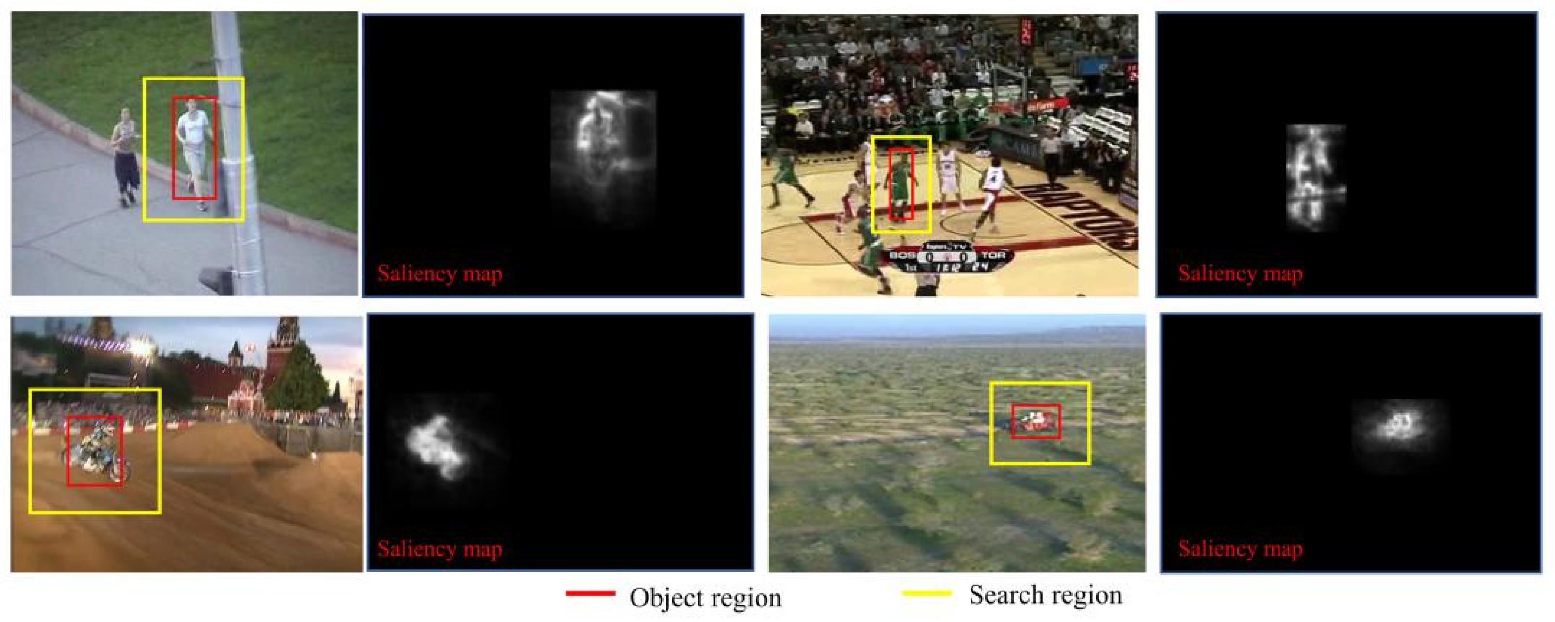
3.2.3. Saliency Detection for Updating Spatial Weights

For the above objective function, in order to address the effect boundary, we attempted to use spatial–temporal regularization to obtain an updated weight map, where the spatial weight $w$ is related. The aim of saliency detection is to identify salient objects and represent their shapes with binary images [31,32,33,34]. For the same purpose, penalizing the background, we exported a saliency map of the target and merged it into the weight map $w$. Then, we simply multiplied the meaning map with the weight map to obtain a new weight map, $w_{new}$, that better reflects the shape of the target.

First, we cropped the search region, which was k times larger than the tracked object, and used an existing saliency detection method [34] to obtain the related saliency map $S_d$; the related saliency detection results are shown in Figure 2. Then, to suppress the effects of the background and let it keep the same size as that of the spatial weight map, we resized $S_d$ into the same size as the CF filter and utilized $S_d$ to regularize the original weight map $w$. Thus, we could obtain the new weight map as follows:

$$w_{new}=S_d\odot w$$

(19)

For online target tracking, a step was previously added to our CF tracking algorithm, using Equation (19) to calculate the weight graph $w_{new}$ of the initial frame, where the target is explained by the bounding box shown. Compared to the above fixed spatial regularization, we introduced an efficient saliency-aware regularized generation method that can adapt to the shape change in objects. Meanwhile, $w$ can result in poor tracking because the influence of its context on the discriminant ability of the training correlation filter is limited. In contrast to $w$, $w_{new}$ is a continuous coordinate function, and by using $w_{new}$ while tracking, the context around the target still makes a contribution toward training discriminative filters.

3.2.4. Object Localization and Scale Estimation

In the process of tracking, we can determine the position of the tracked target by analyzing the correlation response between $\widehat{g}$ of the last frame and the feature map of the search region. The response map formulation is represented as shown below:

$$R(x_k)={\mathcal{F}}^{-1}({\displaystyle \sum _{k=1}^K{\widehat{x}}_k\odot }{\widehat{g}}_k^{v-1})$$

(20)

where $K$ represents the number of channels in the feature map, and ${\widehat{g}}_k^{v-1}$ represents the trained correlation filter from the last frame using the ADMM algorithm in the frequency domain. The maximum response value is defined as the center of the tracked object.

For the scale estimation, inspired by the ASRCF method [15], we trained another scale correlation filter to reduce the computation. Scale-dependent filters are trained with effective HOG features. Next, we selected four scale search regions and obtained the corresponding response maps. We trained the location correlation filters with fused functions, including deep CNN and HOG features. For the CNN features, we chose Conv4-3 of the pretrained VGG-16 [35] model on ImageNet [36]. The scale correlation filter includes HOG features of 31 dimensions, and the location-related correlation filter contains combined HOG and CNN features of 111 dimensions.

Similarly to CF-based trackers, the appearance model is updated as follows:

$${\widehat{X}}_v^{\mathrm{mod}el}=(1-\eta ){\widehat{X}}_{v-1}^{\mathrm{mod}el}+\eta {\widehat{X}}_v$$

(21)

where $v$ and $v-1$ represent the $v$-th and ($v-1$)-th frames, respectively. η is the learning rate of the appearance model. Algorithm 1 shows an explicit process description of the SSTCF method.

Algorithm 1: The proposed tracking algorithm

Input: The initial position $p_0$ and scale size $s_0$ of the object in the initial frame. Output: Estimated object position $p_v$ and scale size $s_v$ in the $v$th frame, tracking model, and CF template. When frame $v=1$, Extract the object features, including the shallow HOG feature and deep CNN feature, and obtain two initial CF templates for object localization and scale estimation, respectively. Initialize parameter $w$; subproblems $h$ and $\widehat{g}$ are calculated utilizing Equations (12) and (17), and subproblems $\widehat{g}$ are updated in three iterations. Compute saliency map $S_d$, and use Equation (19) to obtain the new weight map. When frame $v>1$, repeat: Extract HOG features of 31 dimensions for the scale correlation filter and combine HOG and CNN features of 111 dimensions for the location-related correlation filter. Compute the response $R$ of object localization CF by using Equation (20). The maximum of the responses is the position of the object, and the maximum of the responses in four scale estimation CF is the scale of the object. Update the appearance model using Formulas (21). Compute subproblems $h$ and $\widehat{g}$ by using Equations (12) and (17), and update subproblems $\widehat{g}$ in three iterations. Compute the saliency map $S_d$ and use Equation (19) to obtain the new weight map. End

4. Experimental Results

We implemented our SSTCF methods on the MATLAB 2017a platform using the MatConvNet toolbox on a PC (Lenovo, Beijing, China) equipped with Intel 3.7 GHz and 16 GB RAM with a single NVIDIA GTX 2080ti GPU. For the parameter settings, the regularization parameter was set as ${\lambda }_1=0.2$, the temporal-aware constraint parameter was set as $\beta$ = 15, and the learning rate of the SSTCF was set as $\eta$ = 0.0175. In the ADMM optimization process, we used three iterations, and the penalty factor was set as $\mu$ = 1. The penalty factor at iteration $i+1$ used ${\mu }^{(i+1)}=\min ({\mu }_{\max },\delta {\mu }^{(i)})$ for updating, where $\delta =10$ and ${\mu }_{\max }=1000$.

We used different trackers on three benchmarks to evaluate our method. Our SSTCF method was initially based on the classic short-term datasets OTB2015 [27] and VOT2015, with 100 video sequences, and VOT2015 with 60 video sequences evaluated. We then evaluated the SSTCF tracker on a LaSOT long-term test dataset with 280 sequences, which included many UAV scenes.

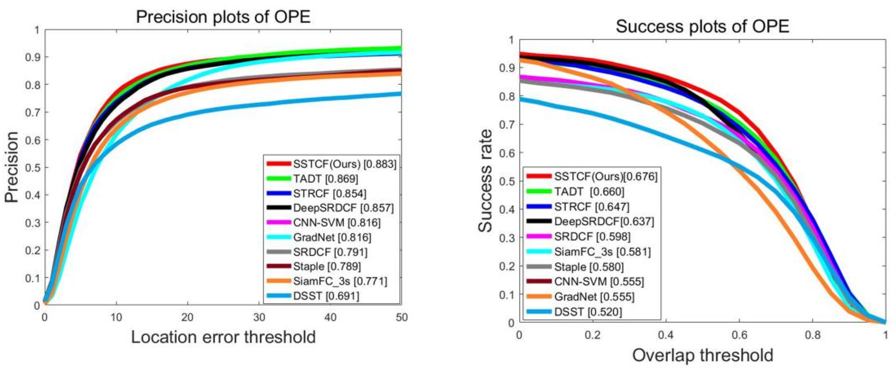
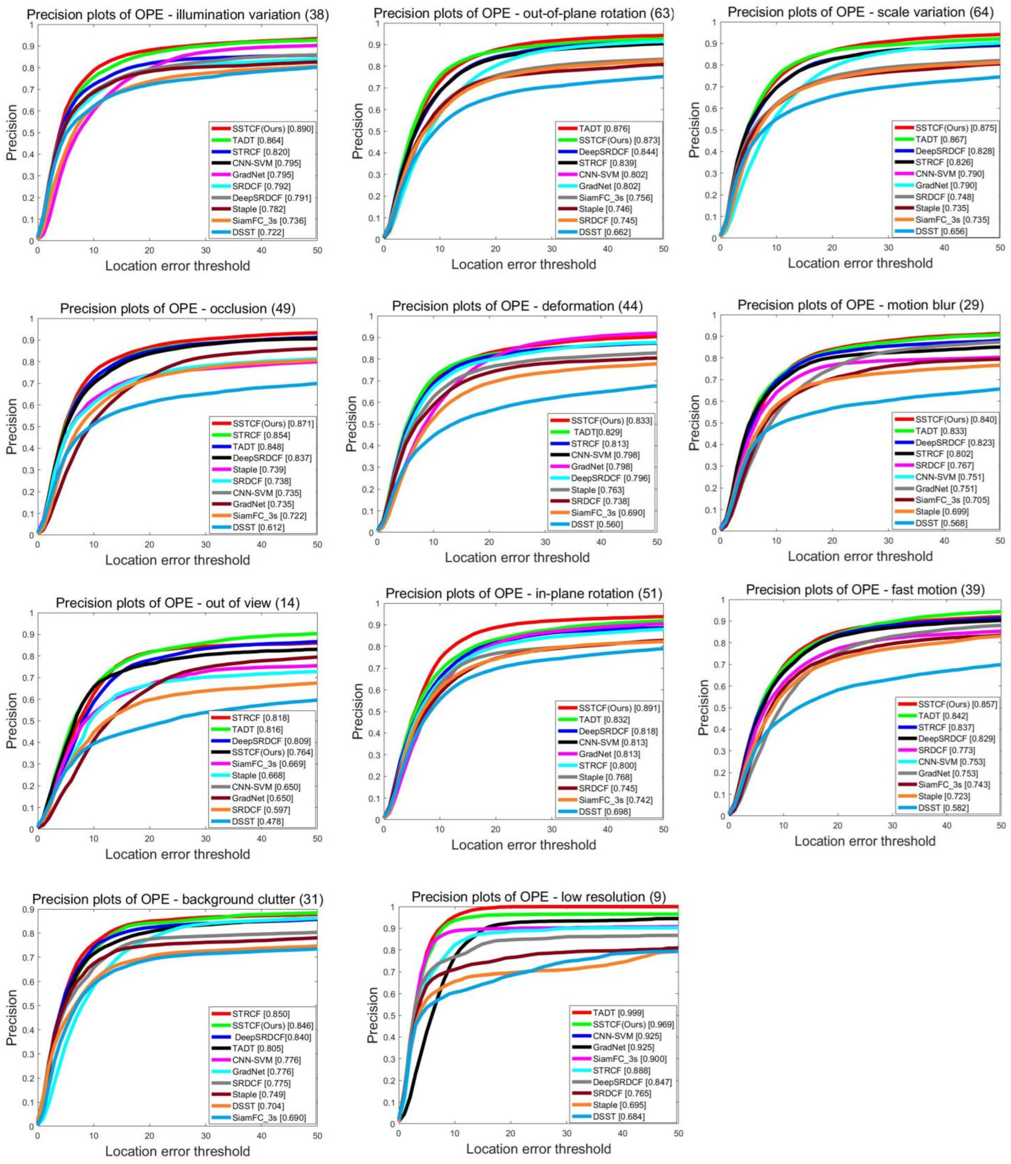
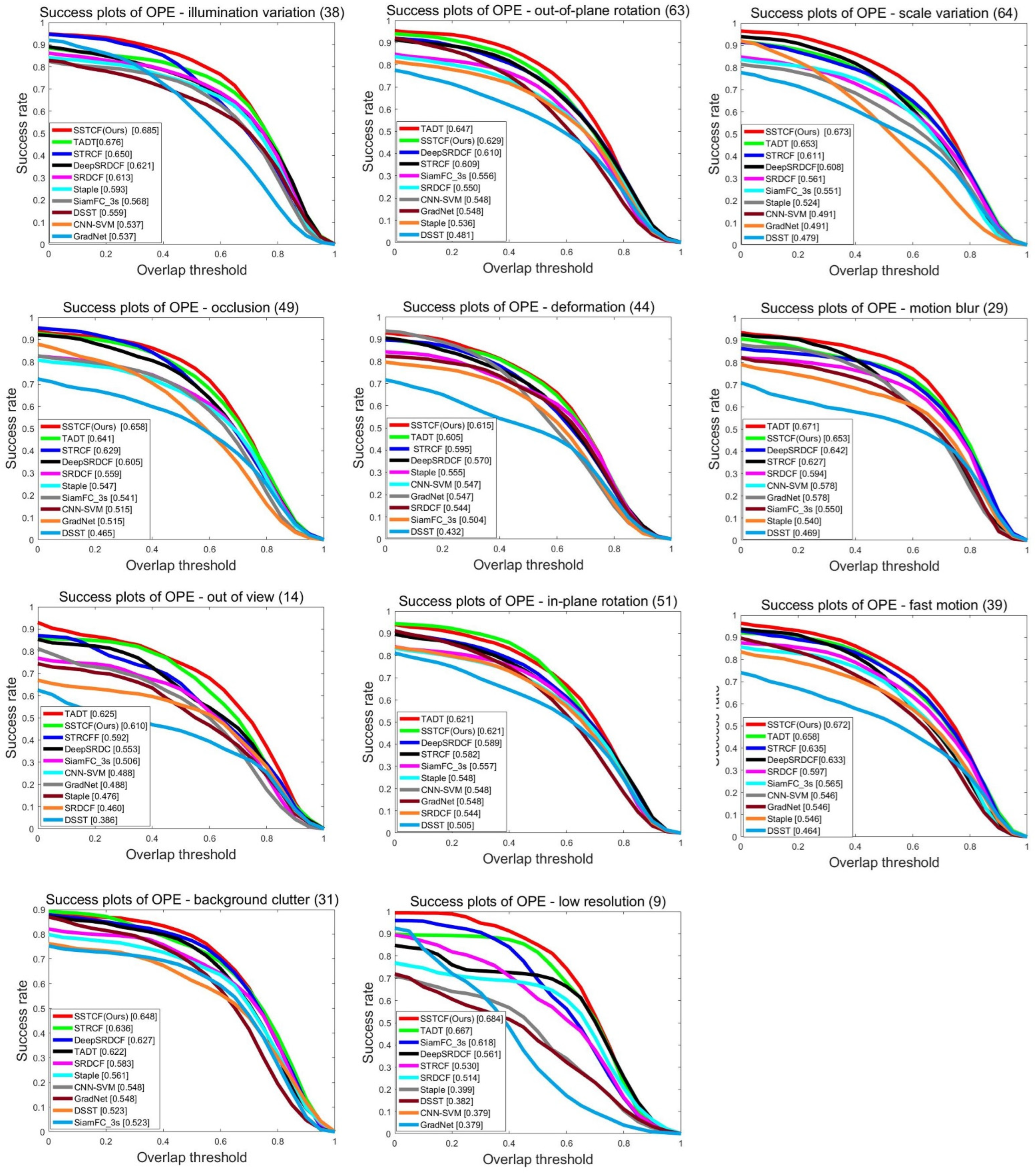
4.1. Evaluation of OTB2015 Dataset

The OTB2015 dataset [27] is a classical dataset in the field of tracking, consisting of 100 video sequences, including low-altitude UAV video, surveillance video, and camera shot video. It is described with eleven different attributes, such as fast motion, occlusion, background clutter, deformation, motion blur, etc. [20]. We evaluated all the trackers using the one-pass evaluation (OPE) protocol, as referred to in [37]. It is used to evaluate the compared trackers with the distance precision and overlap success metrics. We contrasted the SSTCF method with nine existing popular trackers, including those that use hand-crafted and CNN features, such as CNN_SVM [38], GradNet [39], Staple [40], DSST [11], SRDCF [13], DeepSRDCF [23], TADT [41], STRCF [17], and SiamFC [42].

Figure 3 displays the evaluation results of the compared trackers on the OTB2015 dataset [27]. The legends in the accuracy plots represent the mean distance precision (DP) score at 20 pixels, whereas the legends in the success plots represent the area under the curve (AUC) score for each tracker. As can be seen in these plots, our proposed SSTCF method attained sounder results, where the DP score was 0.883, and the AUC score was 0.676. Compared to the baseline STRCF method, our SSTCF tracker improved both the overall DP score and the AUC score by 2.9%. Compared to the SRDCF tracker, our SSTCF performed better; the DP score was improved by 9.2%, and the AUC score was improved by 7.8%. Additionally, our SSTCF tracking method meets the real-time tracking requirement, reaching a tracking speed of 25.1 fps.

Figure 4 and Figure 5 display the precision and success plots of the OPE among ten trackers with eleven video sequence attributions. From the results, we found that our SSTCF tracker performed better than other trackers on most sequence attributions, such as fast motion, occlusion, and deformation. Taking the fast motion attribution as an example, our SSTCF tracker improved the DP score by 1.5% and the AUC score by 1.4% compared to the second-ranking TADT tracker. Based on the experiments on OTB2015, the results verify that our proposed tracker can address complex tracking problems and can also meet the requirements for real-time application.

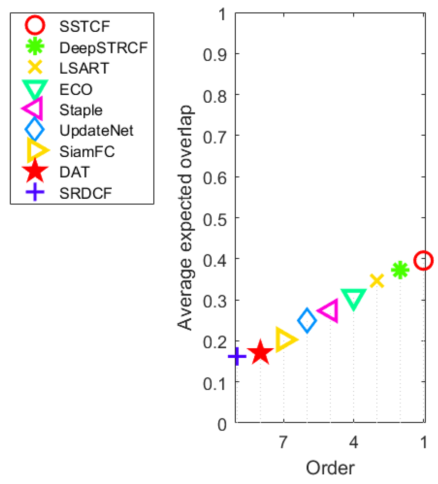
4.2. Evaluation of VOT2018 Dataset

As a visual object tracking (VOT) challenge, the VOT2018 dataset [28] contains 60 challenge sequences. Compared to VOT2017, there were no changes in the evaluation metrics [20], except that ten old sequences were replaced with ten challenge videos. We compared our SSTCF with eight existing popular trackers, including the DSTRCF [17], ECO [43], UpdateNet [44], SRDCF [13], DAT [45], LSART [46], SiamFC [42], and Staple [40]. Following references [20,47], the accuracy, robustness, and expected average overlap (EAO) metrics were utilized in this experiment.

Table 1. Accuracy of nine trackers evaluated on the VOT2018 dataset.

	Camera Motion	Empty	Illum Change	Motion Change	Occlusion	Size Change	Mean	Weighted Mean	Pooled
SSTCF	0.5910	0.5940	0.6010	0.5548	0.4985	0.5018	0.5589	0.5601	0.5763
LSART	0.5470	0.5729	0.5032	0.5071	0.4746	0.4565	0.5102	0.5234	0.5377
DSTRCF	0.4855	0.5499	0.5912	0.4493	0.4322	0.4398	0.4913	0.4866	0.5009
ECO	0.5221	0.5598	0.5253	0.4775	0.3714	0.4436	0.4833	0.4978	0.5130
UpdateNet	0.5226	0.5713	0.5179	0.4936	0.4805	0.4842	0.5117	0.5194	0.5324
SRDCF	0.4855	0.5499	0.5912	0.4493	0.4322	0.4398	0.4913	0.4866	0.5009
Staple	0.5580	0.5958	0.5634	0.5187	0.4764	0.4799	0.5320	0.5405	0.5518
DAT	0.4660	0.4812	0.3388	0.4234	0.3216	0.4382	0.4116	0.4412	0.4492
SiamFC	0.5144	0.5597	0.5683	0.5058	0.4361	0.4675	0.5086	0.5114	0.5165

presents the accuracy outcomes of the eight trackers in nine attributions, including motion change, empty, illumination change, camera motion, occlusion, weighted mean, size change, pooled, and the mean. For the nine attributions, higher scores indicate better performance [20]. Table 1 shows that our SSTCF had superior performance on most attributions compared to the other methods, including motion change, occlusion, and camera motion attributions. The pooled and weighted mean attributions reached 0.5763 and 0.5601, respectively. Additionally,

Table 2. Robustness of nine trackers evaluated on the VOT2018 dataset.

	Camera Motion	Empty	Illum Change	Motion Change	Occlusion	Size Change	Mean	Weighted Mean	Pooled
SSTCF	11.0000	5.0000	1.0000	7.0000	9.0000	6.0000	8.0000	10.0835	33.0000
LSART	16.9333	3.7333	0.5333	8.6667	18.5333	7.7333	9.3556	10.2036	37.0667
DSTRCF	11.0000	11.0000	2.0000	13.0000	10.0000	7.0000	9.0000	10.2551	36.0000
ECO	19.000	7.000	4.000	18.000	18.000	9.000	12.500	13.511	44.000
UpdateNet	29.0000	11.0000	3.0000	33.0000	21.0000	13.0000	18.3333	20.8763	75.0000
SRDCF	52.0000	20.0000	8.0000	47.0000	27.0000	28.0000	30.3333	35.4262	116.0000
Staple	37.0000	24.0000	5.0000	27.0000	36.0000	25.0000	25.6667	28.7784	102.0000
DAT	37.0000	24.0000	5.0000	27.0000	36.0000	25.0000	25.6667	28.7784	102.0000
SiamFC	28.0000	14.0000	5.0000	41.0000	25.0000	22.0000	22.5000	24.6681	90.0000

reports the robustness results of the nine attributions, where the robustness scores indicate the times of failure and lower scores indicate better performance. We can see that our SSTCF model performed well in the robustness scores, especially for motion change, size change, and pooled attributions, which ranked first among all compared trackers. The results of the EAO metrics are presented in Figure 6 and

Table 3. The EAO rank of nine trackers.

Method	All
SSTCF	0.3935
DeepSTRCF	0.3727
LSART	0.3464
ECO	0.3077
Staple	0.2733
UpdateNet	0.2499
SiamFC	0.2029
DAT	0.1709
SRDCF	0.1621

, where higher scores mean better performance. Our SSTCF ranked first among all the trackers. The EAO score was 0.3935, and the EAO score of the second-ranking DeepSTRCF tracker was 0.3727, which is an obvious gap compared to the first-ranking tracker. Therefore, as can be seen from the experiments on the VOT2018 dataset, our SSTCF tracker can effectively handle the challenging situations of visual tracking.

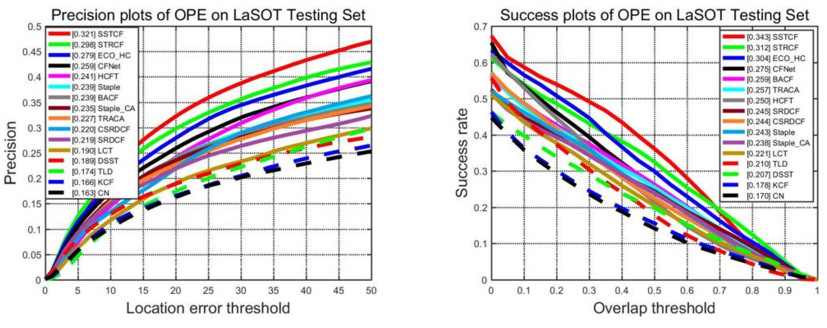
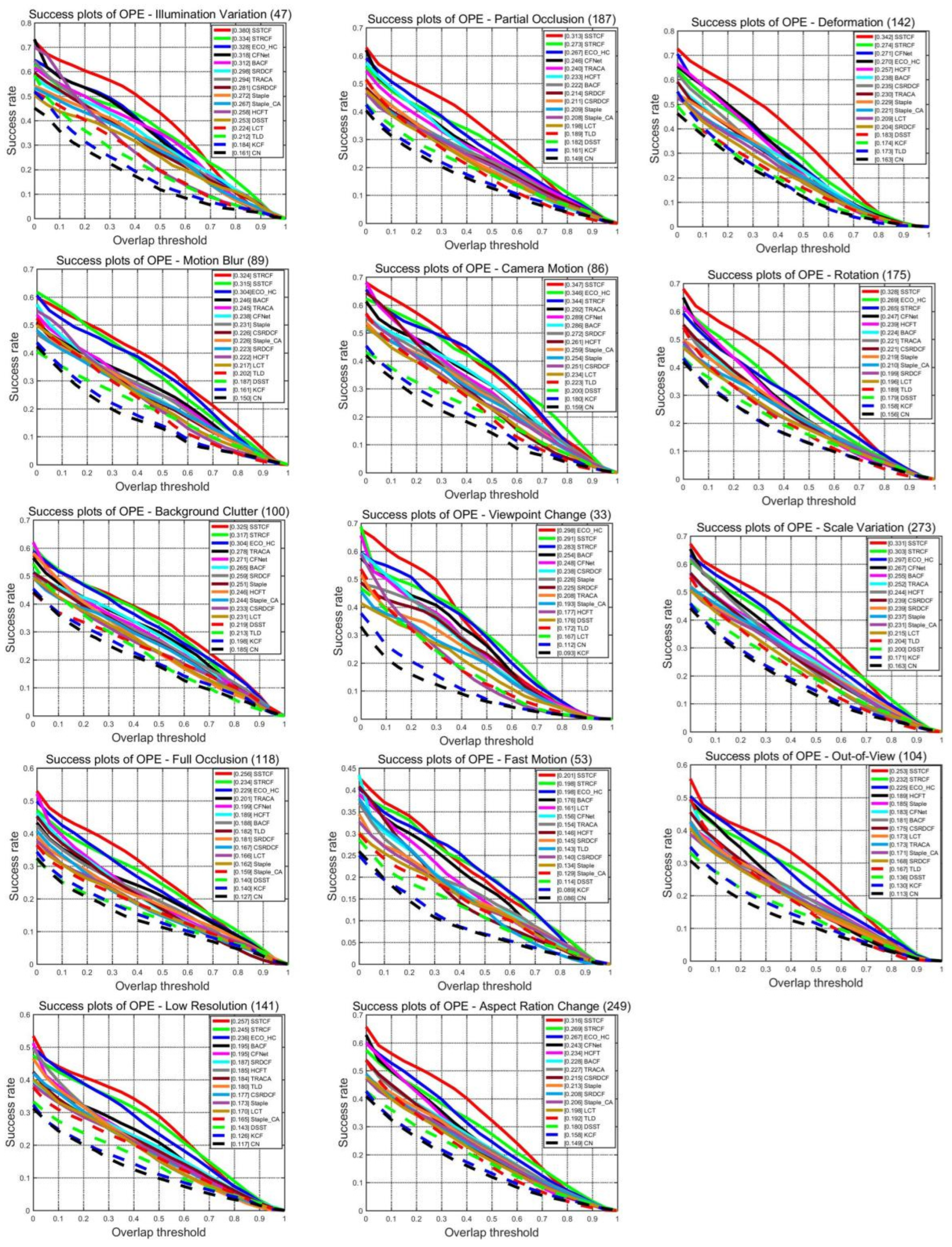
4.3. Evaluate on LaSOT Dataset

The LaSOT dataset [28] is a very large-scale long-term dataset that was released in 2018. We selected a LASOT test set with 280 sequences, with an average image length exceeding 2500 images, with many UAV videos included. In the course of this experiment, we compared the SSTCF with 15 trackers, namely the CSRDCF [48], CFNet [26], ECO_HC [43], HCFT [49], Staple_CA [50], STRCF [17], BACF [14], TRACA [51], Staple [39], LCT [52], SRDCF [13], TLD [53], DSST [11], CN [54], and KCF [10]. For a fair comparison, the evaluation methods also followed the OPE protocol for the different trackers. Success and accuracy plot metrics were employed in this experiment; more detailed descriptions of these measures can be found in [28].

The performance results evaluated using the LaSOT dataset are given in Figure 7. Our SSTCF outperformed the other trackers in both the accuracy and success rates, where the DP score was 0.321 and the AUC score was 0.343. Additionally, we provide the overlap success plots of the 15 compared trackers with 14 different attributes displayed, such as deformation, background clutter, occlusion, etc. The success plots are displayed in Figure 8. It was found that the SSTCF method worked well in all attributes, especially regarding deformation, occlusion, and fast motion attributions, ranking first among all the trackers. Thus, the comparison results evaluated using the LaSOT dataset demonstrate the effectiveness of the SSTCF tracker.

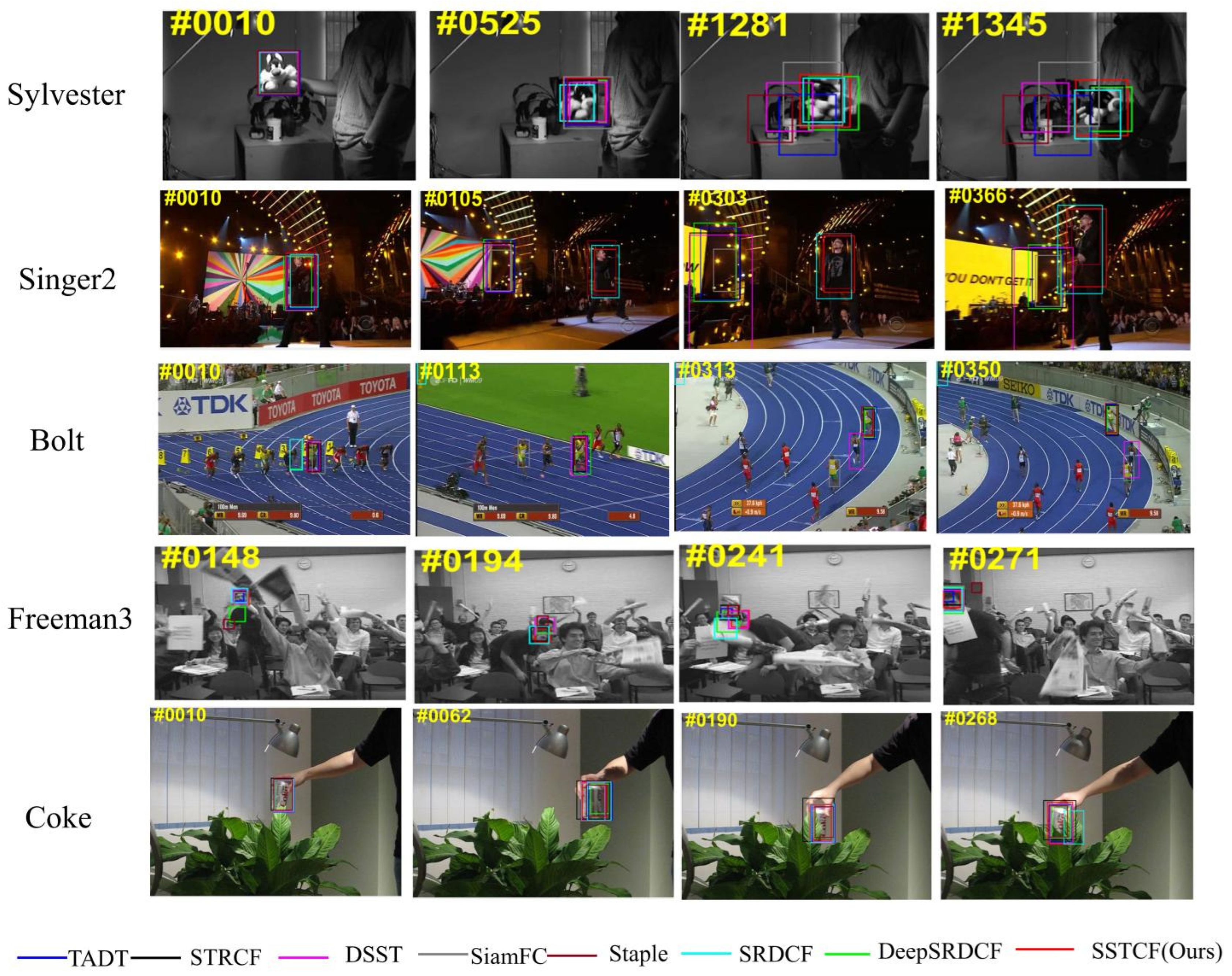
4.4. Qualitative Evaluation

To further intuitively demonstrate the effectiveness of the SSTCF method, we qualitatively evaluated comparative trackers for five representative sequences, including Sylvester, Singer2, Bolt, Freeman3, and Coke. Figure 9 displays the comparison results between the SSTCF and seven existing state-of-the-art trackers: DeepSRDCF [23], STRCF [17], DSST [11], Staple [40], TADT [41], SimaFC [43], and SRDCF [13].

We found that the SSTCF tracker was able to track the objects accurately and consistently, especially objects that had obvious changes, whereas the bounding boxes of some trackers drifted in the tracking process. Taking the Sylvester sequence (including IV, IPR, and OPR attributions) as an example, we found that most trackers could track the object in frame 525, but only a few trackers could maintain the bounding box at the right location, whereas our SSTCF could always track well, even in frame 1345. Therefore, this qualitative evaluation intuitively proves the validity of the recommended tracker.

5. Conclusions

This paper proposes a novel saliency-aware and spatial–temporal regularized correlation filter (SSTCF) model to address unwanted boundary effects and significant appearance changes in challenging UAV video scenarios. The proposed SSTCF method can help build a robust appearance model and improve tracking accuracy by introducing spatial and temporal regularization terms into the objective function. The related objective function was effectively optimized via the ADMM algorithm, greatly reducing the computational cost. Furthermore, the introduced saliency detection method generates new weight to replace the fixed spatial weight, which efficiently adapts to the appearance change and suppresses the background interference. Compared to other trackers, our SSTCF method has shown outstanding performance in most evaluation metrics on multiple benchmarks. We employed various approaches to examine the outcomes of the relevant experiments to demonstrate the effectiveness of the proposed technique. In future endeavors, we will prioritize enhancing the method’s capabilities pertaining to drone scenarios [55].

References

1. Yilmaz, A.; Javed, O.; Shah, M. Object tracking: A survey. ACM Comput. Surv. 2006, 38, 13. [Google Scholar] [CrossRef]
2. Li, P.X.; Wang, D.; Wang, L.J.; Lu, H.C. Deep visual tracking: Review and experimental comparison. Pattern Recognit. 2018, 76, 323–338. [Google Scholar] [CrossRef]
3. Wang, N.Y.; Shi, J.; Yeung, D.Y.; Jia, J. understanding and diagnosing visual tracking systems. In Proceedings of the IEEE International Conference on Computer Vision (ICCV), Santiago, Chile, 7–13 December 2015; pp. 3101–3109. [Google Scholar]
4. Smeulders, A.W.; Chu, D.M.; Cucchiara, R.; Calderara, S.; Dehghan, A. Visual tracking: An experimental survey. IEEE Trans. Pattern Anal. Mach. Intell. 2014, 36, 1442–1468. [Google Scholar] [PubMed]
5. Jang, J.; Jiang, H. MeanShift++: Extremely Fast Mode-Seeking With Applications to Segmentation and Object Tracking. In Proceedings of the IEEE/CVF Conference on Computer Vision and Pattern Recognition (CVPR), Nashville, TN, USA, 20–25 June 2021; pp. 4100–4111. [Google Scholar] [CrossRef]
6. Sundararaman, R.; De Almeida Braga, C.; Marchand, E.; Pettré, J. Tracking Pedestrian Heads in Dense Crowd. In Proceedings of the 2021 IEEE/CVF Conference on Computer Vision and Pattern Recognition (CVPR), Nashville, TN, USA, 20–25 June 2021; pp. 3864–3874. [Google Scholar] [CrossRef]
7. Liu, L.; Cao, J. End-to-end learning interpolation for object tracking in low frame-rate video. IET Image Process. 2020, 14, 1066–1072. [Google Scholar] [CrossRef]
8. Bolme, D.S.; Beveridge, J.R.; Draper, B.A.; Lui, Y.M. Visual object tracking using adaptive correlation filters. In Proceedings of the Twenty-Third IEEE Conference on Computer Vision and Pattern Recognition, CVPR 2010, San Francisco, CA, USA, 13–18 June 2010; pp. 2544–2550. [Google Scholar] [CrossRef]
9. Henriques, J.F.; Caseiro, R.; Martins, P.; Batista, J. Exploiting the Circulant Structure of Tracking-by-Detection with Kernels. In Proceedings of the European Conference on Computer Vision, Florence, Italy, 7–13 October 2012; pp. 702–715. [Google Scholar]
10. Henriques, J.F.; Caseiro, R.; Martins, P.; Batista, J. High-Speed Tracking with Kernelized Correlation Filters. IEEE Trans. Pattern Anal. Mach. Intell. 2015, 37, 583–596. [Google Scholar] [CrossRef] [PubMed]
11. Danelljan, M.; Hager, G.; Khan, F.S.; Felsberg, M. Discriminative Scale Space Tracking. IEEE Trans. Pattern Anal. Mach. Intell. 2017, 39, 1561–1575. [Google Scholar] [CrossRef] [PubMed]
12. Galoogahi, H.K.; Sim, T.; Lucey, S. Correlation Filters with Limited Boundaries. In Proceedings of the 2015 IEEE Conference on Computer Vision and Pattern Recognition (CVPR), Boston, MA, USA, 7–12 June 2015; pp. 4630–4638. [Google Scholar]
13. Danelljan, M.; Hager, G.; Khan, F.S.; Felsberg, M. Learning Spatially Regularized Correlation Filters for Visual Tracking. In Proceedings of the 2015 IEEE International Conference on Computer Vision (ICCV), Santiago, Chile, 7–13 December 2015; pp. 4310–4318. [Google Scholar] [CrossRef]
14. Galoogahi, H.K.; Fagg, A.; Lucey, S. Learning Background-Aware Correlation Filters for Visual Tracking. In Proceedings of the 2017 IEEE International Conference on Computer Vision (ICCV), Venice, Italy, 22–29 October 2017; pp. 1144–1152. [Google Scholar] [CrossRef]
15. Dai, K.; Wang, D.; Lu, H.; Sun, C.; Li, J. Visual Tracking via Adaptive Spatially-Regularized Correlation Filters. In Proceedings of the 2019 IEEE/CVF Conference on Computer Vision and Pattern Recognition (CVPR), Long Beach, CA, USA, 16–20 June 2019; pp. 4665–4674. [Google Scholar] [CrossRef]
16. Boyd, S. Distributed Optimization and Statistical Learning via the Alternating Direction Method of Multipliers. Found. Trends Mach. Learn. 2010, 3, 1–122. [Google Scholar] [CrossRef]
17. Li, F.; Tian, C.; Zuo, W.; Zhang, L.; Yang, M. Learning Spatial-Temporal Regularized Correlation Filters for Visual Tracking. In Proceedings of the 2018 IEEE/CVF Conference on Computer Vision and Pattern Recognition, Salt Lake City, UT, USA, 18–23 June 2018; pp. 4904–4913. [Google Scholar] [CrossRef]
18. Li, Y.; Fu, C.H.; Ding, F.Q.; Huang, Z.Y.; Lu, G. AutoTrack: Towards High-Performance Visual Tracking for UAV With Automatic Spatio-Temporal Regularization. In Proceedings of the 2020 IEEE/CVF Conference on Computer Vision and Pattern Recognition (CVPR), Seattle, WA, USA, 13–19 June 2020; pp. 11920–11929. [Google Scholar] [CrossRef]
19. Han, R.; Feng, W.; Wang, S. Fast Learning of Spatially Regularized and Content Aware Correlation Filter for Visual Tracking. IEEE Trans. Image Process. 2020, 29, 7128–7140. [Google Scholar] [CrossRef]
20. Liu, L.; Feng, T.; Fu, Y. Learning Multifeature Correlation Filter and Saliency Redetection for Long-Term Object Tracking. Symmetry 2022, 14, 911. [Google Scholar] [CrossRef]
21. Zhang, X.; Wang, Z.; Xia, G.; Zhang, L. Accurate object tracking by combining correlation filters and keypoints. In Proceedings of the International Joint Conference on Neural Networks, Vancouver, BC, Canada, 24–29 July 2016. [Google Scholar] [CrossRef]
22. Xie, F.; Wang, C.; Wang, G.; Cao, Y.; Yang, W.; Zeng, W. Correlation-Aware Deep Tracking. In Proceedings of the IEEE/CVF Conference on Computer Vision and Pattern Recognition, New Orleans, LA, USA, 18–24 June 2022. [Google Scholar] [CrossRef]
23. Danelljan, M.; Hager, G.; Khan, F.S.; Felsberg, M. Convolutional Features for Correlation Filter Based Visual Tracking. In Proceedings of the 2015 IEEE International Conference on Computer Vision Workshop (ICCVW), Santiago, Chile, 7–13 December 2015; pp. 621–629. [Google Scholar] [CrossRef]
24. Danelljan, M.; Robinson, A.; Shahbaz, K.F.; Felsberg, M. Beyond Correlation Filters: Learning Continuous Convolution Operators for Visual Tracking; Leibe, B., Matas, J., Sebe, N., Welling, M., Eds.; Computer Vision—ECCV 2016. ECCV 2016. Lecture Notes in Computer Science; Springer: Cham, Switzerland, 2016; Volume 9909. [Google Scholar] [CrossRef]
25. Sun, Y.; Sun, C.; Wang, D.; He, Y.; Lu, H. ROI Pooled Correlation Filters for Visual Tracking. In Proceedings of the 2019 IEEE/CVF Conference on Computer Vision and Pattern Recognition (CVPR), Long Beach, CA, USA, 16–20 June 2019; pp. 5776–5784. [Google Scholar] [CrossRef]
26. Valmadre, J.; Bertinetto, L.; Henriques, J.; Vedaldi, A.; Torr, P.H.S. End-to-End Representation Learning for Correlation Filter Based Tracking. In Proceedings of the 2017 IEEE Conference on Computer Vision and Pattern Recognition (CVPR), Honolulu, HI, USA, 21–26 July 2017; pp. 5000–5008. [Google Scholar] [CrossRef]
27. Wu, Y.; Lim, J.; Yang, M. Object Tracking Benchmark. IEEE Trans. Pattern Anal. Mach. Intell. 2015, 37, 1834–1848. [Google Scholar] [CrossRef] [PubMed]
28. Matej, K.; Ales, L.; Jiri, M.; Michael, F.; Roman, P.; Luka, C.; Tomas, V.; Goutam, B.; Alan, L.; Abdelrahman, E.; et al. The Sixth Visual Object Tracking VOT2018 Challenge Results; Leal-Taixé, L., Roth, S., Eds.; Computer Vision—ECCV 2018 Workshops. ECCV 2018. Lecture Notes in Computer Science; Springer: Cham, Switzerland, 2018; Volume 11129. [Google Scholar] [CrossRef]
29. Fan, H.; Lin, L.; Yang, F.; Chu, P.; Deng, G.; Yu, S.; Bai, H.; Xu, Y.; Liao, C.; Ling, H. LaSOT: A High-Quality Benchmark for Large-Scale Single Object Tracking. In Proceedings of the 2019 IEEE/CVF Conference on Computer Vision and Pattern RECOgnition (CVPR), Long Beach, CA, USA, 16–20 June 2019; pp. 5369–5378. [Google Scholar] [CrossRef]
30. Eckstein, J.; Bertsekas, D.P. On the Douglas—Rachford splitting method and the proximal point algorithm for maximal monotone operators. Math. Program. 1992, 55, 293–318. [Google Scholar] [CrossRef]
31. Feng, W.; Han, R.; Guo, Q.; Zhu, J.; Wang, S. Dynamic saliency-aware regularization for correlation filter-based object tracking. IEEE Trans. Image Process. 2019, 28, 3232–3245. [Google Scholar] [CrossRef] [PubMed]
32. Liu, L.; Cao, J.; Niu, Y. Visual Saliency Detection Based on Region Contrast and Guided Filter. In Proceedings of the 2nd IEEE International Conference on Computational Intelligence and Applications (ICCIA), Beijing, China, 8–11 September 2017; pp. 327–330. [Google Scholar]
33. Yang, X.; Li, S.Y.; Ma, J.; Yang, J.Y.; Yan, J. Co-saliency-regularized correlation filter for object tracking. Signal Process. Image Commun. 2022, 103, 116655. [Google Scholar] [CrossRef]
34. Goferman, S.; Zelnik-Manor, L.; Tal, A. Context-Aware Saliency Detection. IEEE Trans. Pattern Anal. Mach. Intell. 2014, 34, 1915–1926. [Google Scholar] [CrossRef] [PubMed]
35. Karen, S.; Andrew, Z. Very deep convolutional networks for large-scale image recognition. arXiv 2014, arXiv:1409.1556. [Google Scholar]
36. Russakovsky, O.; Deng, J.; Su, H.; Krause, J.; Satheesh, S.; Ma, S.; Huang, Z.; Karpathy, A.; Khosla, A.; Bernstein, M.; et al. Imagenet large scale visual recognition challenge. Int. J. Comput. Vision 2015, 115, 211–252. [Google Scholar] [CrossRef]
37. Wu, Y.; Lim, J.; Yang, M. Online Object Tracking: A Benchmark. In Proceedings of the 2013 IEEE Conference on Computer Vision and Pattern Recognition, Portland, OR, USA, 23–28 June 2013; pp. 2411–2418. [Google Scholar] [CrossRef]
38. Hong, S.; You, T.; Kwak, S.; Han, B. Online tracking by learning discriminative saliency map with convolutional neural network. In Proceedings of the 32nd International Conference on International Conference on Machine Learning, Lile, France, 6–11 July 2015; Volume 37, pp. 597–606. [Google Scholar]
39. Li, P.; Chen, B.; Ouyang, W.; Wang, D.; Yang, X.; Lu, H. GradNet: Gradient-Guided Network for Visual Object Tracking. In Proceedings of the 2019 IEEE/CVF International Conference on Computer Vision (ICCV), Seoul, Republic of Korea, 27 October–2 November 2019; pp. 6161–6170. [Google Scholar] [CrossRef]
40. Bertinetto, L.; Valmadre, J.; Golodetz, S.; Miksik, O.; Torr, P.H.S. Staple: Complementary Learners for Real-Time Tracking. In Proceedings of the 2016 IEEE Conference on Computer Vision and Pattern Recognition (CVPR), Las Vegas, NV, USA, 27–30 June 2016; pp. 1401–1409. [Google Scholar] [CrossRef]
41. Li, X.; Ma, C.; Wu, B.; He, Z.; Yang, M. Target-Aware Deep Tracking. In Proceedings of the 2019 IEEE/CVF Conference on Computer Vision and Pattern Recognition (CVPR), Long Beach, CA, USA, 16–20 June 2019; pp. 1369–1378. [Google Scholar] [CrossRef]
42. Bertinetto, L.; Valmadre, J.; Henriques, J.F.; Vedaldi, A.; Torr, P.H.S. Fully-Convolutional Siamese Networks for Object Tracking; Hua, G., Jégou, H., Eds.; Computer Vision—ECCV 2016 Workshops. ECCV 2016. Lecture Notes in Computer Science; Springer: Cham, Switzerland, 2016; Volume 9914. [Google Scholar] [CrossRef]
43. Danelljan, M.; Robinson, A.; Shahbaz, K.F.; Felsberg, M. ECO: Efficient Convolution Operators for Tracking. In Proceedings of the 2017 IEEE Conference on Computer Vision and Pattern Recognition (CVPR), Honolulu, HI, USA, 21–26 July 2017; pp. 6931–6939. [Google Scholar] [CrossRef]
44. Zhang, L.; Gonzalez-Garcia, A.; Weijer, J.V.D.; Danelljan, M.; Khan, F.S. Learning the Model Update for Siamese Trackers. In Proceedings of the 2019 IEEE/CVF International Conference on Computer Vision (ICCV), Long Beach, CA, USA, 16–20 June 2019; pp. 4009–4018. [Google Scholar] [CrossRef]
45. Possegger, H.; Mauthner, T.; Bischof, H. In defense of color-based model-free tracking. In Proceedings of the 2015 IEEE Conference on Computer Vision and Pattern Recognition (CVPR), Santiago, Chile, 7–13 December 2015; pp. 2113–2120. [Google Scholar] [CrossRef]
46. Sun, C.; Wang, D.; Lu, H.; Yang, M. Learning Spatial-Aware Regressions for Visual Tracking. In Proceedings of the 2018 IEEE/CVF Conference on Computer Vision and Pattern Recognition, Salt Lake City, UT, USA, 18–23 June 2018; pp. 8962–8970. [Google Scholar] [CrossRef]
47. Matej, K.; Jiri, M.; Alexs, L.; Tomas, V.; Roman, P.; Gustavo, F.; Georg, N.; Fatih, P.; Luka, C. A Novel Performance Evaluation Methodology for Single-Target Trackers. IEEE Trans. Pattern Anal. Mach. Intell. 2016, 38, 2137–2155. [Google Scholar] [CrossRef]
48. Lukežic, A.; Vojír, T.; Zajc, L.C.; Matas, J.; Kristan, M. Discriminative Correlation Filter with Channel and Spatial Reliability. In Proceedings of the 2017 IEEE Conference on Computer Vision and Pattern Recognition (CVPR), Honolulu, HI, USA, 21–26 July 2017; pp. 4847–4856. [Google Scholar] [CrossRef]
49. Ma, C.; Huang, J.-B.; Yang, X.; Yang, M.H. Hierarchical Convolutional Features for Visual Tracking. In Proceedings of the 2015 IEEE International Conference on Computer Vision (ICCV), Santiago, Chile, 7–13 December 2015; pp. 3074–3082. [Google Scholar] [CrossRef]
50. Mueller, M.; Smith, N.; Ghanem, B. Context-aware correlation filter tracking. In Proceedings of the IEEE Conference on Computer Vision and Pattern Recognition (CVPR), Honolulu, HI, USA, 21–26 July 2017; pp. 1396–1404. [Google Scholar]
51. Choi, J.; Chang, H.J.; Fischer, T.; Yun, S.; Lee, K.; Jeong, J.; Demiris, Y.; Choi, J.Y. Context-Aware Deep Feature Compression for High-Speed Visual Tracking. In Proceedings of the 2018 IEEE/CVF Conference on Computer Vision and Pattern Recognition, Salt Lake City, UT, USA, 18–23 June 2018; pp. 479–488. [Google Scholar] [CrossRef]
52. Ma, C.; Yang, X.; Zhang, C.Y.; Yang, M. Long-term correlation tracking. In Proceedings of the 2015 IEEE Conference on Computer Vision and Pattern Recognition (CVPR), Santiago, Chile, 7–13 December 2015; pp. 5388–5396. [Google Scholar] [CrossRef]
53. Kalal, Z.; Mikolajczyk, K.; Matas, J. Tracking-Learning-Detection. IEEE Trans. Pattern Anal. Mach. Intell. 2012, 34, 1409–1422. [Google Scholar] [CrossRef] [PubMed]
54. Danelljan, M.; Khan, F.S.; Felsberg, M.; Van De Weijer, J. Adaptive Color Attributes for Real-Time Visual Tracking. In Proceedings of the 2014 IEEE Conference on Computer Vision and Pattern Recognition, Columbus, OH, USA, 23–28 June 2014; pp. 1090–1097. [Google Scholar] [CrossRef]
55. Montoya-Morales, J.R.; Guerrero-Sánchez, M.E.; Valencia-Palomo, G.; Hernández-González, O.; López-Estrada, F.R.; Hoyo-Montaño, J.A. Real-time robust tracking control for a quadrotor using monocular vision. Proc. Inst. Mech. Eng. Part G J. Aerosp. Eng. 2023, 237, 2729–2741. [Google Scholar] [CrossRef]
Figure 1. The overall framework of SSTCF model.
Symmetry 16 01076 g001
Figure 2. Saliency detection in different sequence. The yellow bounding box are the search regions, and red box are object regions.
Symmetry 16 01076 g002
Figure 3. Overall precision plots and success plots of OPE evaluate on the compared trackers.
Symmetry 16 01076 g003
Figure 4. Precision plots of OPE evaluate the compared trackers with eleven sequence attributions.
Symmetry 16 01076 g004
Figure 5. Success plots of OPE evaluate the compared trackers with eleven sequence attributions.
Symmetry 16 01076 g005
Figure 6. The EAO scores rank of all compared trackers. Different markers denote different methods.
Symmetry 16 01076 g006
Figure 7. Precision and success plots of OPE on the LaSOT test set sequences.
Symmetry 16 01076 g007
Figure 8. Success plots of OPE on fourteen sequence attributions.
Symmetry 16 01076 g008
Figure 9. Representative visual tracking results of the compared trackers on five sequences. Red bounding boxes are our results.
Symmetry 16 01076 g009