Abstract
Spin 1/2 quantum spin chains represent the prototypical model for coupled two-level systems. Consequently, they offer a fertile playground for both fundamental and technological applications ranging from the theory of thermalization to quantum computation. Recently, it has been shown that interesting phenomena are associated to the boundary conditions imposed on the quantum spin chains via the so-called topological frustration. In this work, we analyze the effects of such frustration on a few-spin system, with a particular focus on the strong even–odd effects induced in the ground-state energy. We then implement a topologically frustrated quantum spin chain on a quantum computer to show that our predictions are visible on current quantum hardware platforms.
1. Introduction
The theoretical importance and technological potential of coupled multilevel quantum systems are substantial. They range from fundamental issues related to thermalization [1,2,3,4] and information or energy spreading [5] to the realization of quantum bits [6] and quantum batteries [7] and the simulation of complex quantum systems [8]. Within this scenario, a vast amount of interesting physical phenomena in many-body systems have been shown to emerge in frustrated systems [9,10]. Frustration can be induced by both geometric factors [11,12,13] and, as in Wigner crystals [14,15,16,17,18], by interactions [19,20,21]. Recently, a new intriguing kind of frustration has been discovered: Topological Frustration (TF) [22,23]. Qualitatively speaking, TF amounts to the fact that some spin chains with N spins obeying periodic boundary conditions behave very differently, even for large N, depending on the parity of N. Crucially, up to now, topological frustration has only been observed in spin 1/2 systems, hence being a combined effect of topology and quantumness. To understand the physical content of TF, it is useful to start with a very intuitive classical argument: imagine an N site classical antiferromagnetic Ising model in the absence of applied fields, compactified on a circle. If N is even, the lowest energy state is the one with neighbouring spins antiparallel to each other. The degeneracy is twofold: flipping all the spins does not change the energy. If N is odd, on the other hand, it is not possible, due to the boundary conditions, to have all the spins antiparallel to their neighbours. TF is hence at play. The lowest energy state is in this case the one where all spins except for one are antiparallel to their neighbours. The important fact is that the degeneracy of the lowest energy state is now instead of two. At the quantum level, when, for example, a transverse field is switched on, the even N case is characterized in the thermodynamic limit by a gap between the (doubly degenerate) ground state and the excited states. On the other hand, in the odd N case, the system becomes gapless, with the gapless modes originating from the hybridization of the states that are degenerate at the classical point, that is, in the absence of applied fields [24,25]. The implications of this simple observation are complex and far-reaching [22,23,26,27,28,29,30,31,32,33]. Boundary quantum phase transitions that are absent in the even N case show up for odd N, marking the onset of ground states with finite global magnetization in the antiferromagnetic case or the spontaneous breaking of translational invariance [34,35,36]. At the non-equilibrium level, signatures of TF are also visible in the Loschmit echo [29]. Although the best way to take the thermodynamic limit in systems with TF is under intense debate [30,36], what is clear is that systems with finite N presenting TF have a very strong dependence of their properties on the parity of N.
This fact is what we theoretically and experimentally inspect in this work. In particular, we analyze analytically the effects of topological frustration in the XY quantum spin chain with spins. Among other effects, in particular, we show that that the ground-state energy has a way stronger dependence on the applied magnetic field in the presence of TF (antiferromagnetic coupling, odd N) than in the non-frustrated cases. To extend, for the first time, beyond the theoretical description of TF, we then implement a special case of the model discussed theoretically on an IBM quantum computer where the role of the spins is taken by trasmon qubits. Remarkably, we confirm the peculiarity of the system with TF in terms of ground-state energy, with particular reference to the strong even–odd effects it induces.
On one hand, our results confirm the robustness of the physics related to TF in real life contexts, where thermal fluctuations are unavoidable and exact symmetries in the coupling parameters essentially do not exist. On the other hand, they might inspire the conception of nanodevices based on TF, where by only changing N by one, the properties of the system change dramatically. Finally, our work opens the way to experimentally consider topological frustration in quasi one-dimensional setups, where analytical results are hardly achievable [37,38].
The rest of the article is structured as follows. In Section 2, we present and recap the solution of the model. We also discuss the features of topological frustration, resuming some of the most relevant results in the literature so far. In Section 3, we discuss the effects of topological frustration on finite size systems, focusing in particular on the cases. In Section 4 we present our experimental results, and finally in Section 5 we illustrate our conclusions.
2. The XY Model and Its Topological Frustration
2.1. Model
The model under investigation is the so-called XY quantum chain in a transverse field [39,40,41,42,43,44,45,46,47]. The Hamiltonian H is given by
where N is the number of sites, J is the energy scale, is a parameter quantifying the anisotropic way in which nearest neighbour spins interact, h is an external magnetic field along the z direction and (with ) are Pauli matrices in the usual representation. Clearly, we have where is the Kronecker symbol. Crucially for the following, we impose periodic boundary conditions .
We now proceed with the diagonalization of the Hamiltonian. Such diagonalization is well known in the literature [40,41]. Since, however, the TF regime requires some care, we find it worthy to report here the explicit solution.
First of all, thanks to the symmetry properties of (1), we restrict our analysis, without loss of generality, to the first quarter of the parameter space , i.e., . We then introduce the Wigner–Jordan transformation [48], in which the spin operators are non-locally mapped onto spinless fermions. We have
with . The other spin operators are obtained from the commutation relations. Clearly, we have the anticommutation relations with l, m running over the sites of the chain, while all other anticommutation relations between the fermions are zero.
After the transformation, the Hamiltonian H reads
with
the parity operator. We note that the Hamiltonian when written in terms of the fermions is highly non-local and non-linear due to the presence of the operator . Indeed, when expressed in terms of the fermionic operators, such operator reads as However, since , we can decompose the Hamiltonian as
where
In the last equality, we defined
We are now in the position of solving the Hamiltonian. To achieve this, we now switch to Fourier space, with the convention
where
These two sets play a crucial role in the mathematical derivation of even–odd effects in this model.
In Fourier space, we find
Here, we define
where the angle obeys the constraints and
The Hamiltonian now reads
with
This form brings us to the final step of the diagonalization. We have here to distinguish the ferromagnetic case , the most studied one, and the antiferromagnetic case , the one that shows frustration. Note, however, that the Hamiltonians are standard and intensively studied since they represent a topological superconductor [38,49,50,51,52,53,54,55,56,57,58,59].
2.1.1. Ferromagnetic Case
In the ferromagnetic case (), which has been extensively studied [39], it is convenient to chose such that
Furthermore, we introduce the dispersion relation
Note that
From the choice (16), independently from the parity of N, we have
2.1.2. Antiferromagnetic Case
In the antiferromagnetic case (), it is convenient to chose such that
For N even, we have
For N odd, which is the frustrated case and represents the main focus of this work, we have [30]
2.2. Generalities about the Ground State
The physical properties of the ground state and of the low-energy sector in the ferromagnetic and in the antiferromagnetic case can be rather different. Indeed, only the odd N case in the antiferromagnetic regime is affected by TF, i.e., the geometry of the system does not allow us simultaneous minimization of all local interactions in our Hamiltonian (1). This incompatibility between local and global order induces an excitation in the ground state, which becomes gapless in the thermodynamic limit () [24,25], giving rise to the peculiar physics of this system. In this subsection, based on the exact solution just described, we briefly comment on the features of the frustrated XY chain which are independent from the specific (finite) number of sites. For the non-frustrated cases, we also refer to the vast literature [39]. To start, we address the ground state. We call |⟩, |⟩ and |⟩ the most general ground-state elements of, respectively, , and H. We use an analogous notation for the corresponding energy E. Furthermore, we denote with |⟩ the vacuum of fermions . The strategy we adopt to obtain the ground state is the following: identify |⟩; extract |⟩ from the states found in the previous step; find the ground-state energy and, as a consequence, |⟩. In the thermodynamic limit, this algorithm can be realized in a fully analytical way [30,36,39], but at finite N we have to resort to numerical methods.
From Equations (20) and (21), we can see that in the ferromagnetic chain, we have
In the same way, from Equations (23) and (24) in the non-frustrated antiferromagnetic, chain we have
Hence, without frustration, we always have
In other words, when N is even, the ferromagnetic and antiferromagnetic cases are, from the energetic point of view, completely equivalent, with energies given by (31) and (32). It is important to underline that in the absence of frustration, only two states alternate as ground state, with different crossing lines in the first quarter of the parameter space (as we see in the next Section). Furthermore, we can observe from (17) that is an exact degeneracy line for all N. To determine precisely which is the ground state once fixed , we have to compare the energies (31) and (32) [60].
By increasing the number of sites in the frustrated case, we expect that there exists a critical value such that when , the number of regions in the parameter space alternating in z-parity increases [30]. Such expectation is justified by the fact that when (and ), the dispersion relation (17) has the shape in Figure 1, where the minima are at [25]. By increasing N, the cardinality of and increases linearly; as a consequence, by moving in this subregion of the parameter space, we have a more and more frequent change in the elements of and which are closest to [30,36].
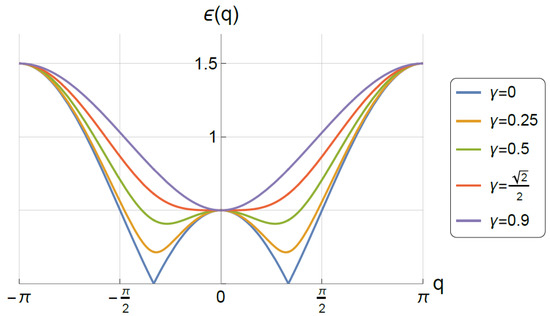
Figure 1.
Plot of the dispersion relation as a function of for and different values of : (blue), (orange), (green), (red) and (purple).
To conclude this introductory section, we observe that at the point , the Hamiltonian (1) reduces to that of the classical Ising chain. As consequence, the ground space in the frustrated case is -fold degenerate and spanned by the “kink states”, which have a single pair of nearest neighbor spins (the kink) that are ferromagnetically aligned in the x direction and the other pairs of nearest neighbor spins antiferromagnetically aligned. Without frustration, the ground space at the classical point is always two times degenerate and spanned by the two Neél states in the antiferromagnetic case and by the two completely x-ferromagnetic states in the ferromagnetic case.
In the next section, we analyze how to address the properties of topological frustration in few-spin systems.
3. Finite Size Effects
In this section, we analyze the finite-size low-energy states of both the frustrated and the the unfrustrated case for and . The aim is to provide testable consequences of topological frustration in finite-size chains. Although we only focus on a few particular values of N, the analysis can be straightforwardly extended to the general values of the number of sites. The analysis we carry out focuses on two main points: the ground-state energy dependence on parameters and the energy gap between the ground state and the excited states, again as a function of close to the classical point. We find that in the frustrated case, the dependence of the ground-state energy on is much more pronounced than in the unfrustrated case. Similarly, the energy gap increases much faster in the frustrated case.
3.1.
The results, which (as already pointed out in the previous Ssction) do not depend on the sign of J, are reported in Figure 2, where we draw in blue the curves of exact double degeneracy of the ground state (where ) and we specify the z-parity of the ground-state vector in the non-degeneracy regions.
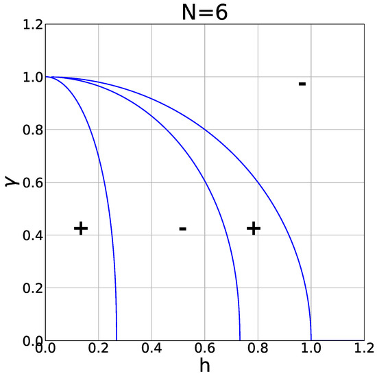
Figure 2.
Double degeneracy curves (in blue) in case for . This plot is independent from the sign of J. The signs + and − specify the z-parity of the (unique) ground state in that region.
From Figure 2, we can see that the neighbourhood of the classical point (where the model reduces to the classical Ising ring) is divided into four regions with alternated z-parities (remember that when or , the ground state is given, respectively, by (29) or (30)), so we expect that the first-order Taylor expansions of and around the classical point are equal. We have
confirmed by the numerical plot shown in Figure 3.
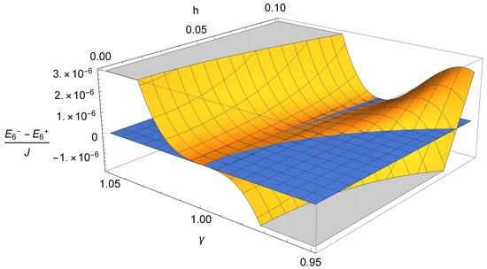
Figure 3.
Numerical plot of around the classical point compared with the plane (in blue). The plot is independent from the value of J.
We also observe that
3.2. Ferromagnetic
The results are reported in Figure 4, where we drawnin blue the curves of exact double degeneracy of the ground state (where ) and we specify the z-parity of the ground-state vector in the non-degeneracy regions.
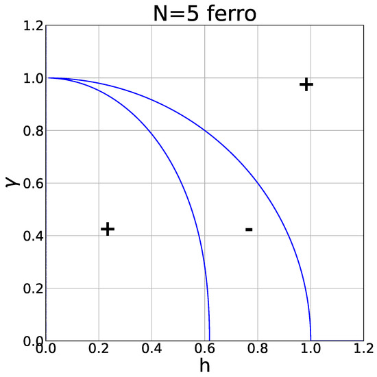
Figure 4.
Double degeneracy curves (in blue) in ferromagnetic case for and . The signs + and − specify the z-parity of the (unique) ground state in that region.
From Figure 4, we can see that the neighbourhood of the classical point is divided in three regions with alternated z-parities, so we expect that the first-order Taylor expansions of and around the classical point are equal (exactly as in the case). The analytic expansion is
confirmed by the numerical plot in Figure 5. We also observe that
As we can see, the behavior is similar to thart in Figure 3 except for the fact that, as already stressed in Section 2.2, the oddness of N implies the exact double degeneracy at .
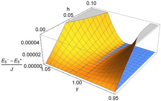
Figure 5.
Numerical plot of in the ferromagnetic case () around the classical point compared with the plane (in blue). The plot is independent from the value of .
3.3. Antiferromagnetic
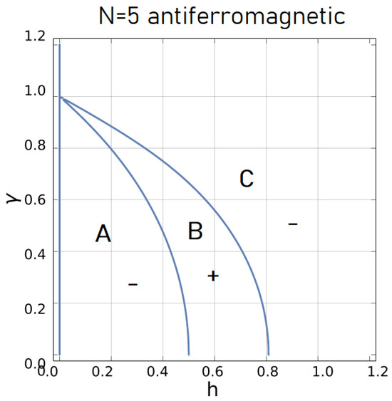
Figure 6.
Degeneracy lines (in blue) in antiferromagnetic case (with ). The letters A, B and C label the three regions with three different ground-state vectors in which the first quarter of the parameter space is divided. As in the even N case, the signs + and − specify the z-parity of the (unique) ground state in that region.
The ground-state energy is
where is the Heaviside step function. Notice that (38) is non-analytical at , having a discontinuity in its first derivative with respect to h (see Figure 7), which survives in the thermodynamic limit, giving birth to a first-order boundary quantum phase transition [35]. On the contrary, this does not happen in the even N antiferromagnetic case and in the even and odd ferromagnetic case, where the ground-state energy (31) is always analytic at , as shown, respectively, in Figure 8 and Figure 9.
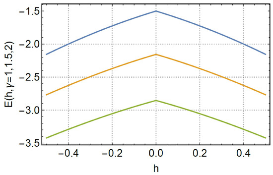
Figure 7.
Ground-state energy E in antiferromagnetic case (with ) as a function of for equal to 1 (blue), 1.5 (orange) and 2 (green).
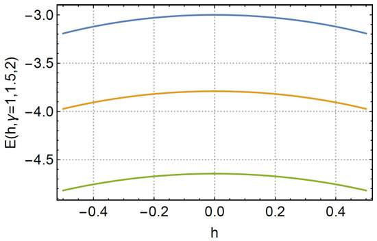
Figure 8.
Ground-state energy E for (with ) as a function of for equal to 1 (blue), 1.5 (orange) and 2 (green). The picture applies to both the ferromagnetic and the antiferromagnetic case.
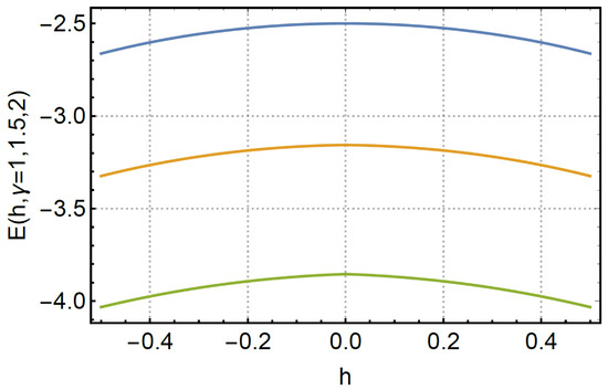
Figure 9.
Ground-state energy E for (with ) in the absence of frustration as a function of for equal to 1 (blue), 1.5 (orange) and 2 (green).
For and , the ground state’s degeneracy is, respectively, 4 and 2 [26,34]. Notice also that at the boundary between regions A and B and regions B and C, the ground state is degenerate, respectively, four and three times.
In the neighbourhood of the classical point with , the different alternating quantum states in the case are three (and given, explicitly, by (37)). The energies of these states which, for the sake of simplicity, we call |A⟩, |B⟩ and |C⟩ (with reference to the subregions of Figure 6), have the following first-order Taylor expansions around the classical point:
where .
4. Implementation on the Quantum Computer
This section addresses the experimental investigation of the effects of topological frustration on the XY chain, for the special choice , which corresponds to the Ising model. In particular, we briefly introduce the technique used to evaluate the physical observables of interests and discuss the outcomes from both numerical simulations and runs on a real IBM quantum device. Namely, we show how to determine the ground state of the Hamiltonian with a variational quantum algorithm and, from there, how to extract its derivative to catch the topological frustration. The first part of extracting the energy of the system is actually very well known and discussed in the literature of quantum computation, with several examples of efficient techniques and hardware-specific characterization. What has been covered least is the possibility of extracting precise values, for small values of the magnetic field, of discontinuities in the derivative. This requires a very precise estimation of the ground state together with a smart choice in its the discrete difference window.
4.1. Variational Quantum Eigensolver
The Variational Quantum Eigensolver (VQE) [61] is a hybrid quantum-classical variational algorithm that produces an upper-bound estimate of the ground-state and its energy of a Hamiltonian H [62]. Based on the Rayleigh–Ritz variational principle, it has found ubiquitous application in fields ranging from quantum chemistry [63] to nuclear physics [64] and many-body physics [65]. The algorithm is actually hybrid, involving both quantum and classical operations. More specifically, VQE proceeds according to the following workflow:
- An ansatz wavefunction is prepared on a quantum computer through a parametric quantum circuit;
- The energy for the given ansatz is evaluated ;
- The set of parameters specifying the state, here generically indicated with , is updated in order to minimize the energy through a classical optimization routine.
The choice of the ansatz is crucial for the whole algorithm to work properly. The employed must indeed meet a reasonable tradeoff between expressivity and trainability: a great number of parameters certainly allows representation of more diverse wavefunctions (including the optimal one), but can significantly slow down the minimization process. Being a Parametrized Quantum Circuit (PQC), it could be characterized by barren plateaus where the gradient becomes exponentially small in the number of qubits during the training. Here, not only the choice of the ansätze is important, but also the initialization strategy of its parameters deserves a theoretical discussion for practical applications [66].
There is a huge amount of literature for specific use cases; here, we cite two approaches to potential design strategy: physically motivated ones [67,68], which are usually difficult to implement on near-term quantum devices, and hardware-efficient ansätze (HEA) [69] that are devised to limit the consequences of noise.
As for the present work, a heuristic trial wavefunction consisting of layered , i.e., rotation, and gates is employed and the optimization procedure is carried out through a stochastic gradient descent (SGD) method named SPSA [70]. The whole implementation is performed within Qiskit [71] framework.
4.2. Ideal Simulations and Results
We start our investigation by leveraging ideal simulations of the finite-size model, noiseless setups serving as a perfect benchmark to explore the possible extension of the study to real device runs. For this reason, we consider the Hamiltonian
for qubits and periodic boundary conditions. We consider the and cases separately and evaluate the ground-state energy for . The VQE procedure is started from a two-layers ansatz as the one shown in Figure 10 with random initial parameters.
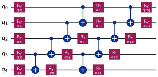
Figure 10.
Example of ansatz for the VQE algorithm. Single-qubit rotation gates are intertwined with entangling gates in a sequence of circuit layers. The angles of the rotations represent the free parameters to be optimized during the minimization procedure. Linear entanglement, with gates acting on adjacent qubits, is preferred to a fully entangled ansatz in order to speed up the computation time.
The approximate values of at each minimization step for every choice of and h are reported in Figure 11. The VQE algorithm in the absence of decoherence is found to display a good and fast convergence to the exact ground-state energies, represented by dotted lines and obtained through an exact diagonalization of the full Hamiltonian.
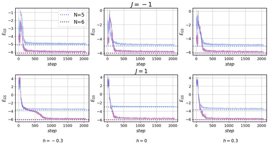
Figure 11.
Estimated during a 2000-step optimization procedure with SPSA for both and . Dotted lines refer to the exact ground-state energies.
In light of evaluating the derivative difference , we consider the output of the VQE algorithm as displayed in Figure 12 for a small deviation of the magnetic field from the null value both for the ferromagnetic and the antiferromagnetic case.
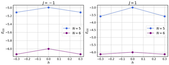
Figure 12.
obtained through VQE as a function of the magnetic field h for each realization of J and N.
Using forward difference to compute numerical derivatives (Table 1), we find satisfactory agreement with analytical predictions regarding both numerical values and the role of J in determining the behavior of for even and odd values of N.

Table 1.
Derivative differences obtained from noiseless simulations.
4.3. Superconducting Quantum Device Results
In the following, we show and discuss results obtained from a superconducting transmon IBM Quantum chip. Starting from encouraging preliminary results, in terms of performance and evaluation of in the previously described noiseless scenario, we extend our analysis further by analyzing stability and reproducibility in a real context, where a real, noisy quantum computer is used, and where state-of-the-art error suppression techniques are exploited. The quantum device used in this work, namely ibm-cairo (Falcon ) consists of 27 fixed-frequency transmons qubits, with fundamental transition frequencies of approximately 5 GHz and anharmonicities of MHz. Microwave pulses are used for single-qubit gates and cross-resonance interaction for two-qubit gates. The experiments take place without intermediate calibration using IBM Qiskit Primitive Estimator. This way, the quantum platform computes the expectation values of the observable (the energy in this case) with respect to the states prepared by the PQC and which can be optimized using the same classical gradient descent-based algorithm as for the noiseless scenario. The topology of the deployed device is displayed in Figure 13. According to the Hamiltonian we study, consisting of 5, 6 qubits, respectively, we map every site of it to a physical qubit, without further recompilation. The connectivity of the physical model is enough to match the requirement of the spin model under evaluation, since the IBM device provides a square topology that is repeated and forms the final 27-qubit layout. In the case of a fully connected model, these kinds of chips require more care in the final mapping, sometimes suggesting the possibility of working with a different quantum technology. However, state-of-the-art superconducting chips displays very good performance to allow execution of the quantum circuit up to dozens of qubits and circuit depths.
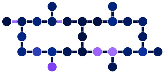
Figure 13.
Schematic representation of the topology of the 27-qubit ibm-cairo device on which computations are performed. Calibration data at the time of running are: Median T1: 89.55 μs, Median T2: 98.7 μs, Median CNOT error: and Median readout error: .
In the case of computation on a quantum hardware, it is essential to consider the adverse effects of noise and devise methods to reduce them. For this reason, the previous VQE routine is supplemented with error mitigation techniques (EM) that are readily provided in the Qiskit environment. In particular, we employ Twisted Readout Error eXtinction (TREX) [72] and Dynamical Decoupling (DD) [73]. TREX is a model-free approach to readout errors that result in biases in quantum expectation values as the ones we are interested in. By randomizing the output channel of a circuit through the application of random bit flips prior to measurements, the estimation bias is turned into a multiplicative factor that can be readily divided out. In addition, DD exploits properly tuned control pulses to average environment-induced decoherence to zero, thus contributing to the clean out of the final result. Similarly to the noiseless case, the approximate values of as the function of the minimization steps for each choice of and h are shown in Figure 14.
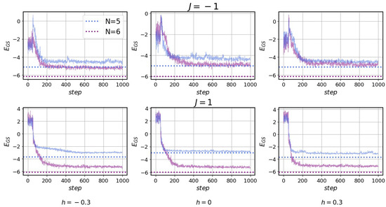
Figure 14.
Estimated in a 1000-step optimization process for both and . Dashed lines refer to the exact ground-state energies. The number of steps of each optimization procedure is varied in each case.
As one could expect from the very beginning, the optimization procedure on the quantum platform yields less favorable outcomes than the ideal case, with convergence being achieved at values slightly distant from the exact ones. Nonetheless, repeating the protocol used for the ideal simulations, we obtain what is shown in Figure 15, where the noiseless results are displayed for completeness.
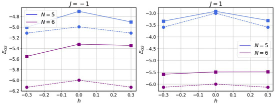
Figure 15.
obtained through VQE as a function of the magnetic field h for each realization of J and N. Circles and squares, respectively, refer to noiseless simulations and real hardware runs.
In an analogy to the ideal case, the derivative difference is evaluated using the finite difference method.
Although decoherence affects the VQE algorithm leading to evaluations of , which significantly differs from the exact ones, especially for qubits (Figure 15), the results reported in Table 2 align satisfactorily with the ones obtained in the noiseless setup, allowing the capture of the emergence of the quantum phase transition even on real hardware.
Table 2.
Derivative differences obtained from runs on the real IBM hardware.
5. Conclusions
After a detailed presentation of the solution of the XY model, we compared its low-energy states with and without frustrated boundary conditions. We found that the ground-state energy and the gap to the lowest lying excited states exhibit a stronger dependence on the parameters of the Hamiltonian when the system is frustrated. We then studied experimentally the Ising chain, a special case of the XY model, implementing the Hamiltonian for different values of the magnetic field with and without frustration for on an IBM Quantum computer. Our results confirmed the theoretical ones, hence demonstrating the possibility of actually implementing topological frustration on quantum computers.
Author Contributions
A.F.M. and F.R.D.F. equally contributed to the experimental results (Section 4), D.S.S. wrote the theoretical introduction (Section 2 and Section 3), N.T.Z., M.S. and M.G. equally contributed to the idealization. All authors took part in the interpretation of the results and in writing the manuscript. All authors have read and agreed to the published version of the manuscript.
Funding
N.T.Z. acknowledges the funding through the NextGenerationEu Curiosity Driven Project “Understanding even-odd criticality”. N.T.Z. and M.S. acknowledge the funding through the “Non-reciprocal supercurrent and topological transitions in hybrid Nb-InSb nanoflags” project (Prot. 2022PH852L) in the framework of PRIN 2022 initiative of the Italian Ministry of University (MUR) for the National Research Program (PNR). M.G. is supported by CERN through CERN Quantum Technology Initiative. Access to IBM devices was obtained through the CERN Quantum HUB at CERN.
Data Availability Statement
Data is contained within the article.
Conflicts of Interest
The authors declare no conflicts of interest.
References
- Vidmar, L.; Rigol, M. Generalized Gibbs ensemble in integrable lattice models. J. Stat. Mech. Theory Exp. 2016, 2016, 064007. [Google Scholar] [CrossRef]
- Abanin, D.A.; Altman, E.; Bloch, I.; Serbyn, M. Colloquium: Many-body localization, thermalization, and entanglement. Rev. Mod. Phys. 2019, 91, 021001. [Google Scholar] [CrossRef]
- Porta, S.; Cavaliere, F.; Sassetti, M.; Traverso Ziani, N. Topological classification of dynamical quantum phase transitions in the xy chain. Sci. Rep. 2020, 10, 12766. [Google Scholar] [CrossRef]
- Porta, S.; Gambetta, F.M.; Traverso Ziani, N.; Kennes, D.M.; Sassetti, M.; Cavaliere, F. Nonmonotonic response and light-cone freezing in fermionic systems under quantum quenches from gapless to gapped or partially gapped states. Phys. Rev. B 2018, 97, 035433. [Google Scholar] [CrossRef]
- Bose, S. Quantum communication through spin chain dynamics: An introductory overview. Contemp. Phys. 2007, 48, 13–30. [Google Scholar] [CrossRef]
- Posske, T.; Thorwart, M. Winding Up Quantum Spin Helices: How Avoided Level Crossings Exile Classical Topological Protection. Phys. Rev. Lett. 2019, 122, 097204. [Google Scholar] [CrossRef]
- Ferraro, D.; Campisi, M.; Andolina, G.M.; Pellegrini, V.; Polini, M. High-Power Collective Charging of a Solid-State Quantum Battery. Phys. Rev. Lett. 2018, 120, 117702. [Google Scholar] [CrossRef]
- Toskovic, R.; van den Berg, R.; Spinelli, A.; Eliens, I.S.; van den Toorn, B.; Bryant, B.; Caux, J.S.; Otte, A.F. Atomic spin-chain realization of a model for quantum criticality. Nat. Phys. 2016, 12, 656–660. [Google Scholar] [CrossRef]
- Ramirez, A.P. Strongly Geometrically Frustrated Magnets. Annu. Rev. Mater. Res. 1994, 24, 453–480. [Google Scholar] [CrossRef]
- Introduction to Frustrated Magnetism: Materials, Experiments, Theory; Springer: Berlin/Heidelberg, Germany, 2011.
- Seo, M.; Choi, H.K.; Lee, S.Y.; Kim, N.; Chung, Y.; Sim, H.S.; Umansky, V.; Mahalu, D. Charge Frustration in a Triangular Triple Quantum Dot. Phys. Rev. Lett. 2013, 110, 046803. [Google Scholar] [CrossRef]
- Sakai, A.; Lucas, S.; Gegenwart, P.; Stockert, O.; Löhneysen, H.v.; Fritsch, V. Signature of frustrated moments in quantum critical CePd1-xNixAl. Phys. Rev. B 2016, 94, 220405. [Google Scholar] [CrossRef]
- König, E.J.; Coleman, P.; Komijani, Y. Frustrated Kondo impurity triangle: A simple model of deconfinement. Phys. Rev. B 2021, 104, 115103. [Google Scholar] [CrossRef]
- Meyer, J.S.; Matveev, K.A. Wigner crystal physics in quantum wires. J. Phys. Condens. Matter 2008, 21, 023203. [Google Scholar] [CrossRef]
- Gambetta, F.M.; Ziani, N.T.; Cavaliere, F.; Sassetti, M. Correlation functions for the detection of Wigner molecules in a one-channel Luttinger liquid quantum dot. Europhys. Lett. 2014, 107, 47010. [Google Scholar] [CrossRef][Green Version]
- Traverso Ziani, N.; Fleckenstein, C.; Dolcetto, G.; Trauzettel, B. Fractional charge oscillations in quantum dots with quantum spin Hall effect. Phys. Rev. B 2017, 95, 205418. [Google Scholar] [CrossRef]
- Shapir, I.; Hamo, A.; Pecker, S.; Moca, C.P.; Legeza, Ö.; Zarand, G.; Ilani, S. Imaging the electronic Wigner crystal in one dimension. Science 2019, 364, 870–875. [Google Scholar] [CrossRef] [PubMed]
- Ziani, N.T.; Cavaliere, F.; Becerra, K.G.; Sassetti, M. A Short Review of One-Dimensional Wigner Crystallization. Crystals 2021, 11, 20. [Google Scholar] [CrossRef]
- Zhitomirsky, M.E.; Ueda, K. Valence-bond crystal phase of a frustrated spin-1/2 square-lattice antiferromagnet. Phys. Rev. B 1996, 54, 9007–9010. [Google Scholar] [CrossRef]
- Capriotti, L.; Sorella, S. Spontaneous Plaquette Dimerization in the J1–J2 Heisenberg Model. Phys. Rev. Lett. 2000, 84, 3173–3176. [Google Scholar] [CrossRef]
- Wang, L.; Poilblanc, D.; Gu, Z.C.; Wen, X.G.; Verstraete, F. Constructing a Gapless Spin-Liquid State for the Spin-1/2J1–J2 Heisenberg Model on a Square Lattice. Phys. Rev. Lett. 2013, 111, 037202. [Google Scholar] [CrossRef]
- Giampaolo, S.M.; Ramos, F.B.; Franchini, F. The frustration of being odd: Universal area law violation in local systems. J. Phys. Commun. 2019, 3, 081001. [Google Scholar] [CrossRef]
- Torre, G.; Odavić, J.; Fromholz, P.; Giampaolo, S.M.; Franchini, F. Long-range entanglement and topological excitations. arXiv 2023, arXiv:2310.16091. [Google Scholar] [CrossRef]
- Dong, J.J.; Li, P.; Chen, Q.H. The a-cycle problem for transverse Ising ring. J. Stat. Mech. Theory Exp. 2016, 2016, 113102. [Google Scholar] [CrossRef]
- Dong, J.J.; Li, P. The a-cycle problem in XY model with ring frustration. Mod. Phys. Lett. B 2017, 31, 1750061. [Google Scholar] [CrossRef]
- Marić, V.; Giampaolo, S.M.; Kuić, D.; Franchini, F. The frustration of being odd: How boundary conditions can destroy local order. New J. Phys. 2020, 22, 083024. [Google Scholar] [CrossRef]
- Marić, V.; Giampaolo, S.M.; Franchini, F. Fate of local order in topologically frustrated spin chains. Phys. Rev. B 2022, 105, 064408. [Google Scholar] [CrossRef]
- Torre, G.; Marić, V.; Franchini, F.; Giampaolo, S.M. Effects of defects in the XY chain with frustrated boundary conditions. Phys. Rev. B 2021, 103, 014429. [Google Scholar] [CrossRef]
- Torre, G.; Marić, V.; Kuić, D.; Franchini, F.; Giampaolo, S.M. Odd thermodynamic limit for the Loschmidt echo. Phys. Rev. B 2022, 105, 184424. [Google Scholar] [CrossRef]
- Catalano, A.G.; Brtan, D.; Franchini, F.; Giampaolo, S.M. Simulating continuous symmetry models with discrete ones. Phys. Rev. B 2022, 106, 125145. [Google Scholar] [CrossRef]
- Odavić, J.; Haug, T.; Torre, G.; Hamma, A.; Franchini, F.; Giampaolo, S.M. Complexity of frustration: A new source of non-local non-stabilizerness. SciPost Phys. 2023, 15, 131. [Google Scholar] [CrossRef]
- Catalano, A.G.; Giampaolo, S.M.; Morsch, O.; Giovannetti, V.; Franchini, F. Frustrating quantum batteries. arXiv 2023, arXiv:2307.02529. [Google Scholar] [CrossRef]
- Marić, V.; Torre, G.; Franchini, F.; Giampaolo, S.M. Topological Frustration can modify the nature of a Quantum Phase Transition. SciPost Phys. 2022, 12, 075. [Google Scholar] [CrossRef]
- Marić, V.; Giampaolo, S.M.; Franchini, F. Quantum phase transition induced by topological frustration. Commun. Phys. 2020, 3, 220. [Google Scholar] [CrossRef]
- Sacco Shaikh, D.; Sassetti, M.; Traverso Ziani, N. Parity-Dependent Quantum Phase Transition in the Quantum Ising Chain in a Transverse Field. Symmetry 2022, 14, 996. [Google Scholar] [CrossRef]
- Shaikh, D.S.; Catalano, A.G.; Cavaliere, F.; Franchini, F.; Sassetti, M.; Ziani, N.T. Phase diagram of the topologically frustrated XY chain. EPJ Plus 2024, 139, 743. [Google Scholar] [CrossRef]
- Faure, Q.; Takayoshi, S.; Petit, S.; Simonet, V.; Raymond, S.; Regnault, L.P.; Boehm, M.; White, J.S.; Månsson, M.; Rüegg, C.; et al. Topological quantum phase transition in the Ising-like antiferromagnetic spin chain BaCo2V2O8. Nat. Phys. 2018, 14, 716–722. [Google Scholar] [CrossRef]
- Traverso, S.; Sassetti, M.; Traverso Ziani, N. Emerging topological bound states in Haldane model zigzag nanoribbons. Npj Quantum Mater. 2024, 9, 9. [Google Scholar] [CrossRef]
- Franchini, F. An Introduction to Integrable Techniques for One-Dimensional Quantum Systems; Springer International Publishing: Berlin/Heidelberg, Germany, 2017. [Google Scholar] [CrossRef]
- Katsura, S. Statistical Mechanics of the Anisotropic Linear Heisenberg Model. Phys. Rev. 1962, 127, 1508–1518. [Google Scholar] [CrossRef]
- Lieb, E.; Schultz, T.; Mattis, D. Two soluble models of an antiferromagnetic chain. Ann. Phys. 1961, 16, 407–466. [Google Scholar] [CrossRef]
- Niemeijer, T. Some exact calculations on a chain of spins 12. Physica 1967, 36, 377–419. [Google Scholar] [CrossRef]
- Niemeijer, T. Some exact calculations on a chain of spins 12 II. Physica 1968, 39, 313–326. [Google Scholar] [CrossRef][Green Version]
- Basor, E.L.; Tracy, C.A. The Fisher-Hartwig conjecture and generalizations. Phys. A Stat. Mech. Appl. 1991, 177, 167–173. [Google Scholar] [CrossRef]
- Izergin, A.G.; Its, A.R.; Korepin, V.E.; Slavnov, N.A. Integrable differential equations for temperature correlation functions of the XXO Heisenberg chain. J. Math. Sci. 1996, 80, 1747–1759. [Google Scholar] [CrossRef]
- Its, A.R.; Izergin, A.G.; Korepin, V.E.; Slavnov, N.A. Temperature correlations of quantum spins. Phys. Rev. Lett. 1993, 70, 1704–1706. [Google Scholar] [CrossRef]
- Grazi, R.; Shaikh, D.S.; Sassetti, M.; Ziani, N.T.; Ferraro, D. Enhancing energy storage crossing quantum phase transitions in an integrable spin quantum battery. arXiv 2024, arXiv:2402.09169. [Google Scholar]
- Jordan, P.; Wigner, E. Über das Paulische Äquivalenzverbot. Z. Phys. 1928, 47, 631–651. [Google Scholar] [CrossRef]
- Kitaev, A.Y. Unpaired Majorana fermions in quantum wires. Phys.-Uspekhi 2001, 44, 131. [Google Scholar] [CrossRef]
- Law, K.T.; Lee, P.A.; Ng, T.K. Majorana Fermion Induced Resonant Andreev Reflection. Phys. Rev. Lett. 2009, 103, 237001. [Google Scholar] [CrossRef]
- Akhmerov, A.R.; Dahlhaus, J.P.; Hassler, F.; Wimmer, M.; Beenakker, C.W.J. Quantized Conductance at the Majorana Phase Transition in a Disordered Superconducting Wire. Phys. Rev. Lett. 2011, 106, 057001. [Google Scholar] [CrossRef]
- San-Jose, P.; Lado, J.L.; Aguado, R.; Guinea, F.; Fernández-Rossier, J. Majorana Zero Modes in Graphene. Phys. Rev. X 2015, 5, 041042. [Google Scholar] [CrossRef]
- Peñaranda, F.; Aguado, R.; Prada, E.; San-Jose, P. Majorana bound states in encapsulated bilayer graphene. SciPost Phys. 2023, 14, 075. [Google Scholar] [CrossRef]
- Haim, A.; Berg, E.; von Oppen, F.; Oreg, Y. Signatures of Majorana Zero Modes in Spin-Resolved Current Correlations. Phys. Rev. Lett. 2015, 114, 166406. [Google Scholar] [CrossRef]
- Fleckenstein, C.; Ziani, N.T.; Calzona, A.; Sassetti, M.; Trauzettel, B. Formation and detection of Majorana modes in quantum spin Hall trenches. Phys. Rev. B 2021, 103, 125303. [Google Scholar] [CrossRef]
- Pakizer, J.D.; Matos-Abiague, A. Signatures of topological transitions in the spin susceptibility of Josephson junctions. Phys. Rev. B 2021, 104, L100506. [Google Scholar] [CrossRef]
- Nadj-Perge, S.; Drozdov, I.K.; Li, J.; Chen, H.; Jeon, S.; Seo, J.; MacDonald, A.H.; Bernevig, B.A.; Yazdani, A. Observation of Majorana fermions in ferromagnetic atomic chains on a superconductor. Science 2014, 346, 602–607. [Google Scholar] [CrossRef]
- Jeon, S.; Xie, Y.; Li, J.; Wang, Z.; Bernevig, B.A.; Yazdani, A. Distinguishing a Majorana zero mode using spin-resolved measurements. Science 2017, 358, 772–776. [Google Scholar] [CrossRef]
- Ziani, N.T.; Fleckenstein, C.; Vigliotti, L.; Trauzettel, B.; Sassetti, M. From fractional solitons to Majorana fermions in a paradigmatic model of topological superconductivity. Phys. Rev. B 2020, 101, 195303. [Google Scholar] [CrossRef]
- De Pasquale, A.; Facchi, P. XY model on the circle: Diagonalization, spectrum, and forerunners of the quantum phase transition. Phys. Rev. A 2009, 80, 032102. [Google Scholar] [CrossRef]
- Peruzzo, A.; McClean, J.; Shadbolt, P.; Yung, M.H.; Zhou, X.Q.; Love, P.J.; Aspuru-Guzik, A.; O’Brien, J.L. A variational eigenvalue solver on a photonic quantum processor. Nat. Comm. 2014, 5, 4213. [Google Scholar] [CrossRef]
- Westerheim, H.; Chen, J.; Holmes, Z.; Luo, I.; Nuradha, T.; Patel, D.; Rethinasamy, S.; Wang, K.; Wilde, M.M. Dual-VQE: A quantum algorithm to lower bound the ground-state energy. arXiv 2023, arXiv:2312.03083. [Google Scholar]
- Crippa, L.; Tacchino, F.; Chizzini, M.; Aita, A.; Grossi, M.; Chiesa, A.; Santini, P.; Tavernelli, I.; Carretta, S. Simulating Static and Dynamic Properties of Magnetic Molecules with Prototype Quantum Computers. Magnetochemistry 2021, 7, 117. [Google Scholar] [CrossRef]
- Dumitrescu, E.F.; McCaskey, A.J.; Hagen, G.; Jansen, G.R.; Morris, T.D.; Papenbrock, T.; Pooser, R.C.; Dean, D.J.; Lougovski, P. Cloud Quantum Computing of an Atomic Nucleus. Phys. Rev. Lett. 2018, 120, 210501. [Google Scholar] [CrossRef]
- Grossi, M.; Kiss, O.; De Luca, F.; Zollo, C.; Gremese, I.; Mandarino, A. Finite-size criticality in fully connected spin models on superconducting quantum hardware. Phys. Rev. E 2023, 107, 024113. [Google Scholar] [CrossRef]
- Grant, E.; Wossnig, L.; Ostaszewski, M.; Benedetti, M. An initialization strategy for addressing barren plateaus in parametrized quantum circuits. Quantum 2019, 3, 214. [Google Scholar] [CrossRef]
- Stetcu, I.; Baroni, A.; Carlson, J. Variational approaches to constructing the many-body nuclear ground state for quantum computing. Phys. Rev. C 2022, 105, 064308. [Google Scholar] [CrossRef]
- Kiss, O.; Grossi, M.; Lougovski, P.; Sanchez, F.; Vallecorsa, S.; Papenbrock, T. Quantum computing of the 6Li nucleus via ordered unitary coupled clusters. Phys. Rev. C 2022, 106, 034325. [Google Scholar] [CrossRef]
- Kandala, A.; Mezzacapo, A.; Temme, K.; Takita, M.; Brink, M.; Chow, J.M.; Gambetta, J.M. Hardware-efficient variational quantum eigensolver for small molecules and quantum magnets. Nature 2017, 549, 242–246. [Google Scholar] [CrossRef]
- Spall, J. Implementation of the simultaneous perturbation algorithm for stochastic optimization. IEEE Trans. Aerosp. Electron. Syst. 1998, 34, 817–823. [Google Scholar] [CrossRef]
- Qiskit Contributors. Qiskit: An Open-source Framework for Quantum Computing. Zenodo 2023. [Google Scholar] [CrossRef]
- van den Berg, E.; Minev, Z.K.; Temme, K. Model-free readout-error mitigation for quantum expectation values. Phys. Rev. A 2022, 105, 032620. [Google Scholar] [CrossRef]
- Ezzell, N.; Pokharel, B.; Tewala, L.; Quiroz, G.; Lidar, D.A. Dynamical decoupling for superconducting qubits: A performance survey. arXiv 2023, arXiv:2207.03670. [Google Scholar] [CrossRef]


Disclaimer/Publisher’s Note: The statements, opinions and data contained in all publications are solely those of the individual author(s) and contributor(s) and not of MDPI and/or the editor(s). MDPI and/or the editor(s) disclaim responsibility for any injury to people or property resulting from any ideas, methods, instructions or products referred to in the content. |
© 2024 by the authors. Licensee MDPI, Basel, Switzerland. This article is an open access article distributed under the terms and conditions of the Creative Commons Attribution (CC BY) license (https://creativecommons.org/licenses/by/4.0/).