Investigation of Analytical Soliton Solutions to the Non-Linear Klein–Gordon Model Using Efficient Techniques

Abstract

Nonlinear distinct models have wide applications in various fields of science and engineering. The present research uses the mapping and generalized Riccati equation mapping methods to address the exact solutions for the nonlinear Klein–Gordon equation. First, the travelling wave transform is used to create an ordinary differential equation form for the nonlinear partial differential equation. This work presents the construction of novel trigonometric, hyperbolic and Jacobi elliptic functions to the nonlinear Klein–Gordon equation using the mapping and generalized Riccati equation mapping methods. In the fields of fluid motion, plasma science, and classical physics the nonlinear Klein–Gordon equation is frequently used to identify of a wide range of interesting physical occurrences. It is considered that the obtained results have not been established in prior study via these methods. To fully evaluate the wave character of the solutions, a number of typical wave profiles are presented, including bell-shaped wave, anti-bell shaped wave, W-shaped wave, continuous periodic wave, while kink wave, smooth kink wave, anti-peakon wave, V-shaped wave and flat wave solitons. Several 2D, 3D and contour plots are produced by taking precise values of parameters in order to improve the physical description of solutions. It is noteworthy that the suggested techniques for solving nonlinear partial differential equations are capable, reliable, and captivating analytical instruments.

1. Introduction

Mathematicians, engineers, physicists, and many other experts have been observed nonlinear problems in the past. The nonlinear evolution equations (NLEEs) are now being studied in a variety of nonlinear fields including protein chemistry, applied mathematics, physics [1], geochemistry, chemical kinematics, meteorology, mathematical fluid dynamics [2], plasma physics [3], and the propagation of shallow water waves. There is a growing interest in the work on soliton wave solutions of NLEEs. Since these NLEEs are mathematical representations of the phenomena, finding the exact solutions to these models will be helpful in our understanding of the phenomena. These equations are used to model physical processes that change over time as well as to explain how systems behave over time. Additionally, complex structures and systems like diffusion, fracture, and turbulence are examined using NLEEs.

The precise solutions to nonlinear partial differential equations (NLPDEs) can be found using a variety of significant and efficient methods [4]. Many physical and scientific problems in nature are illustrated by differential equations. Precise solutions for traveling wave differential equations are essential for utilizing these nonlinear phenomena. Significant progress has been achieved by mathematicians in developing numerous methods for solving NLPDEs. Nonlinear physical sciences obtain particularly from exact solutions since they enable an analysis of the problem’s physical behavior and the investigation of other aspects that may have an impact on the future [5].

The NLEEs are a type of mathematical equation used to describe how a system changes over time. An NLPDE is a specific type of equation that combines the ideas of nonlinearity and describes change across multiple variables. While most NLPDEs are notoriously difficult to solve, a special class known as integrable NLPDEs offers a glimmer of hope. These equations, despite their complexity, possess a surprising property: they can be solved using more manageable techniques compared to the general case. This integrability allows researchers to find exact solutions or analyze properties that would be intractable for typical NLPDEs. Some prominent examples of integrable NLEEs include the Korteweg–de Vries (KdV) equation, crucial for understanding shallow water waves and solitons; the NLS equation, with applications in diverse fields like nonlinear optics and Bose–Einstein condensates; and the sine-Gordon equation, relevant in condensed matter and high-energy physics for studying solitons and kink waves.

Furthermore, a recent review on another NLEE of the nonlinear Schrödinger (NLS) equation reveals that it can be derived not only from the KdV equation but also from a nonlinear Klein–Gordon (KG) equation [6]. The author also highlighted an immense range of applications of the NLS equation and its ability to simulate wave packet dynamics in various fields, including hydrodynamics, nonlinear optics, superconductivity, and Bose-Einstein condensates.

For exact solutions of NLEEs including the fractional low-pass electrical transmission line model, the Korteweg–de Vries (KdV) equation, three coupled nonlinear Maccari systems, the generalized sine-Gordon equation, a variant of the Boussinesq equation, the generalized $(2+1)$-dimensional NLPDE the the extended direct algebraic method [7], the extended trial equation method [8], the truncated Painlevé technique [9] and the modified hyperbolic function expansion method [10] are quite helpful. The exact three-soliton solutions of a third-order nonlinear Schrödinger equation are obtained using the Hirota’s bilinear approach, as indicated in [11]. As stated in [12], the analytical investigation of three-soliton interactions with various phases in nonlinear optics is obtained using Hirota’s bilinear approach.

Nonlinear mathematical modeling has been demonstrated to be a valuable field of study for researchers and scientists. This resulted in the development and enhancement of several important and practical methods for solving problems, such as the modified rational sine-cosine method [13], Hirota bilinear transformation [14], double $({\displaystyle \frac{G^{\prime }}{G}},{\displaystyle \frac{1}{G}})$-expansion method [15,16], the spectral collocation technique [17], the generalized unified approach [18], the inverse scattering transform technique [19], the extended tanh-function method [20], sine-Gordon expansion approach [21], the Kudryashov approach [22,23,24], the new auxiliary equation method [25], the Sardar sub-equation method [26], the modified and generalized Kudryashov method [27,28], the exp-function method [29], the homotopy perturbation method [30], the conservation law scheme [31], the modified $({\displaystyle \frac{G^{\prime }}{G}})$-expansion approach [32] and the orthogonal Lie algebra scheme [33] and others.

The new perturbation iteration transform method, as described in [34], is used to solve linear and nonlinear Klein–Gordon (KG) equations. Traveling wave solutions are found for the non-linear time fractional KG and sine-Gordon equations through an extended tanh-function approach as given in [35]. As stated in [36], analytical and numerical solutions are found for the KG model with cubic nonlinearity. The utilization of the perturbation iteration techniques described in [37] yields novel approximate solutions to the nonlinear KG equations. Solve the KG and sine-Gordon equations using the homotopy-perturbation approach as described in [38]. The numerical solution of the generalized nonlinear KG equation, as provided in [39], is found using a new trigonometric spline approach. Ref. [40] provides an instance of the hybrid cubic B-spline collocation method for solving a generalized nonlinear KG equation. The nonlinear KG problem may be solved using the dual reciprocity boundary integral equation approach, as described in [41].

The mapping and generalized Riccati equation mapping (GREM) methods are used in this research to find the exact solutions of KG model. In [42], the solitons and other solutions for two nonlinear Schrödinger equations using the novel mapping technique. The Biswas–Arshed model’s optical solitons utilizing the mapping approach are provided in [43]. In [44], the mapping approach is used to address soliton solutions in optical metamaterials. Soliton solutions of the $(4+1)$-dimensional Davey–Stewartson–Kadomtsev–Petviashvili equation via modified extended mapping method are derived in [45]. The improved GREM technique for the perturbed nonlinear Chen–Lee–Liu dynamical equation is used in [46]. In [47], the GREM method is utilized to analyze the reaction-diffusion Lengyel–Epstein system analytically. The modified GREM approach is presented in [48] for the investigation of Brownian motion in stochastic Schrödinger wave equation. The modified GREM approach is applied to investigate the cmZKB and pZK equations, as described in [49]. In [50], the generalized nonlinear Schrödinger equation with logarithmic nonlinearity is examined as a template for optical pulse transmission.

The objective of this article is to generalize the exact solutions by applying the mapping and GREM methods for the well-known nonlinear KG model [51,52],

$$v_{tt}(r,t)-{\lambda }^2{v}_{rr}(r,t)+\alpha v(r,t)-\beta v^2(r,t)=0,$$

(1)

where $v_{tt}(r,t)={\displaystyle \frac{{\partial }^{2}v(r,t)}{\partial t^2}}$, $v_{rr}(r,t)={\displaystyle \frac{{\partial }^{2}v(r,t)}{\partial r^2}}$, $v(r,t)$ describes the particle-wave profile, $\lambda$ represents the second-order spatial dispersion and the coefficient of quadratic nonlinearity is represented by $\beta$. From the analysis of each term and traveling wave variable $\zeta =ar-\psi t$, it is clear that Equation (1) is Lorentz-invariant. The transmission of disruption and the Bloch wall activity of magnets in crystals, magnetic flux on a Josephson line, a “splay wave” through a membrane, and many other scientific applications are examples of how the KG model is applied in relativistic quantum fields. The KG equation is encountered in many scientific fields, including nonlinear optics, solid-state physics, and quantum field theory. In relativistic quantum mechanics, which describes spinless particles, this equation is very important. In addition, there has been a lot of interest in soliton-like structures recently. As they propagate, soliton waves do not cause any deformation from dispersion.

Our primary goal in this research is to use the mapping and GREM approaches to find the exact solutions to Equation (1). These commonly used mathematical techniques enable us to do time-consuming and complex algebraic computations quickly and easily. The results show that compared to the alternative approaches, the mapping and GREM procedures are more accurate and need less computing power. The forms of hyperbolic and trigonometric functions for the GREM approach as well as hyperbolic and Jacobi elliptic functions via the mapping method are derived, with a large range of free parameter values. These methods yield diverse soliton solutions including bell-shaped waves, anti-bell-shaped waves, W-shaped waves, continuous periodic waves, kink waves, smooth kink waves, anti-peakon waves, V-shaped waves and flat wave solitons. In addition to improving our understanding of the physical phenomena that NLEEs depict, the work shows the robustness of the mapping and GREM techniques by clearly deriving a variety of soliton solutions as implications of the variables in the NLEEs. In-depth $2D$ and $3D$ graphical representations of the solutions are included in the research to help with a better understanding of their physical characteristics and to demonstrate how well the suggested approach works for solving complex nonlinear equations. The mapping and GREM methods have not yet been used to find the exact solution for the non-linear KG equation. The exact solutions to the non-linear KG equation have been extracted for the inaugural time using these methods. This encourages us to solve the KG equation using these techniques.

The work of this paper is arranged in the following manner. Section 2 provides a description of the procedure for solving NLPDEs by the mapping and GREM methods. However, Section 3 shows these approaches can be used to solve the nonlinear Klein–Gordon Model. Section 4 presents the graphical representation. In Section 5, the conclusion is given.

2. Description of Exact Approaches

This section presents the algorithm for obtaining the exact solutions of NLPDE by using the mapping and GREM methods. These methods are explained below:

2.1. Mapping Method

The following is the fundamental concept of the mapping method. Suppose a given NLPDE in two variables r and t.

$$H(v,v_r,v_t,v_{rr},v_{tt},v_{rt},\dots )=0,$$

(2)

where $v=v(r,t)$ is an unknown function, and H is a polynomial in v and its partial derivatives, in which the highest order derivatives and nonlinear terms are involved.

Step 1. Using the wave-transformation relation, Equation (2) can be converted into the ordinary differential equation (ODE). The wave transformation is as follows:

$$v(r,t)=V(\zeta ),\zeta =ar-\psi t,$$

(3)

where a and $\psi$ are the wave number and velocity, respectively. By inserting Equation (3) in Equation (2), the NLPDE is converted into the following ODE,

$$H(V,V^{\prime },V^{″},V^{‴},\dots )=0,$$

(4)

where H is a polynomial in $V(\zeta )$ with derivatives of $V(\zeta )$ and the prime represents the derivative with regard to $\zeta$ such that $V^{\prime }(\zeta )={\displaystyle \frac{dV}{d\zeta }}$, $V^{″}(\zeta )={\displaystyle \frac{d^{2}V}{d{\zeta }^2}}$ and so on. If Equation (4) is integrable, then take each integral constant to be zero and integrate it as many times as needed.

Step 2. Assume that Equation (4) has the formal solution,

$$V(\zeta )=\sum _{j=1}^k{\eta }_j{g}^j(\zeta ),$$

(5)

where k is a positive integer that needs to be calculated and ${\eta }_j$ are real constants such that ${\eta }_k\ne 0$ to be identified, while $g(\zeta )$ satisfies the elliptic equation of the first kind

$$\left\{\begin{array}{c}{g}^{″}=\gamma g+\delta g^3,\hfill \\ g^{\prime 2}=\gamma g^2+{\displaystyle \frac{1}{2}}\delta g^4+\rho ,\hfill \end{array}\right.$$

(6)

where the prime denotes the derivative with respect to $\zeta$ and $\gamma$, $\delta$, $\rho$ are three arbitrary parameters.

Step 3. The number k depends upon the higher order derivative in Equation (3) and the power of the nonlinearity in Equation (2).

Step 4. Now substitute Equation (5) along with Equation (6) into Equation (4), equalize each of $g^j(\zeta )$ coefficients to zero, producing a system of algebraic equations that Mathematica 12 can solve to determine the values of ${\eta }_j$.

Step 5. The Equation (6) generates the following solutions, for real solutions, $\gamma$ and $\delta$ should be of opposite signs.

$$\left\{\begin{array}{c}g(\zeta )=tanh(\zeta ),\hfill \\ g(\zeta )=sech(\zeta ),\hfill \\ g(\zeta )=\mathrm{sn}(\zeta ),org(\zeta )=\mathrm{cd}(\zeta ),\hfill \\ g(\zeta )=\mathrm{cn}(\zeta ),\hfill \\ g(\zeta )=\mathrm{dn}(\zeta ),\hfill \\ g(\zeta )=\mathrm{ns}(\zeta ),org(\zeta )=\mathrm{dc}(\zeta ),\hfill \end{array}\right.$$

(7)

where $g(\zeta )=\mathrm{sn},\mathrm{cd},\mathrm{cn},\mathrm{dn},\mathrm{ns},\mathrm{dc}$ are Jacobi elliptic functions. The Equation (6) is considered, because solitary waves are obtained by sech-function and shock waves are obtained by tanh-function. However, the periodic waves in terms of Jacobi elliptic functions $g(\zeta )=\mathrm{sn},\mathrm{cd},\mathrm{cn},\mathrm{dn},\mathrm{ns},\mathrm{dc}$ are obtained for appropriate values of the parameters $\gamma$, $\delta$ and $\rho$. The Jacobi elliptic functions $\mathrm{sn}=\mathrm{sn}(\zeta |b)$, $\mathrm{cd}=\mathrm{cd}(\zeta |b)$, $\mathrm{cn}=\mathrm{cd}(\zeta |b)$, $\mathrm{dn}=\mathrm{dn}(\zeta |b)$, $\mathrm{ns}=\mathrm{ns}(\zeta |b)$, $\mathrm{dc}=\mathrm{dc}(\zeta |b)$ where b are double periodic, have the modulus of the elliptic function and have particular properties with triangular functions, such as:

$$\left\{\begin{array}{c}{\mathrm{sn}}^2(\zeta )+{\mathrm{cn}}^2(\zeta )=1,\hfill \\ {\mathrm{dn}}^2(\zeta )+b^2{\mathrm{sn}}^2(\zeta )=1,\hfill \\ \mathrm{sn}{(\zeta )}^{\prime }=\mathrm{cn}(\zeta )\mathrm{dn}(\zeta ),\hfill \\ \mathrm{cn}{(\zeta )}^{\prime }=-\mathrm{sn}(\zeta )\mathrm{dn}(\zeta ),\hfill \\ \mathrm{dn}{(\zeta )}^{\prime }=-b^2\mathrm{sn}(\zeta )\mathrm{cn}(\zeta ).\hfill \end{array}\right.$$

When $b\to 0$, the Jacobi elliptic functions deform to the triangular functions, i.e.,

$$\left\{\begin{array}{c}\mathrm{sn}(\zeta )\to sin(\zeta ),\hfill \\ \mathrm{cn}(\zeta )\to cos(\zeta ),\hfill \\ \mathrm{dn}(\zeta )\to 1.\hfill \end{array}\right.$$

When $b\to 1$, the Jacobi elliptic functions deform to the hyperbolic functions, i.e.,

$$\left\{\begin{array}{c}\mathrm{sn}(\zeta )\to tanh(\zeta ),\hfill \\ \mathrm{cn}(\zeta )\to sech(\zeta ),\hfill \\ \mathrm{dn}(\zeta )\to sech(\zeta ).\hfill \end{array}\right.$$

2.2. Generalized Riccati Equation Mapping Method

It is possible to obtain the exact solutions for the NLPDE by employing the GREM method. Suppose that an NLPDE has the following form

$$H(v,v_r,v_t,v_{rr},v_{tt},v_{rt},\dots )=0,$$

(8)

where $v=v(r,t)$ is an unknown function, and H is a polynomial in v and its partial derivatives, in which the highest order derivatives and nonlinear terms are involved.

Step 1. Using the wave-transformation relation, the Equation (8) can be converted into ODE. The wave transformation is as follows:

$$v(r,t)=V(\zeta ),\zeta =ar-\psi t,$$

(9)

where a and $\psi$ are the wave number and velocity, respectively. By inserting Equation (9) in Equation (8), the NLPDE is converted into the following ODE,

$$H(V,V^{\prime },V^{″},V^{‴},\dots )=0,$$

(10)

where H is a polynomial in $V(\zeta )$ with derivatives of $V(\zeta )$ and the prime represents the derivative with regard to $\zeta$ such that $V^{\prime }(\zeta )={\displaystyle \frac{dV}{d\zeta }}$, $V^{″}(\zeta )={\displaystyle \frac{d^{2}V}{d{\zeta }^2}}$ and so on. If Equation (10) is integrable, then take each integral constant as zero and integrate it as many times as needed.

Step 2. Suppose that Equation (10) has the formal solution

$$V(\zeta )=\sum _{j=-k}^k{\sigma }_j{G}^j(\zeta ),$$

(11)

where k is a positive integer that needs to be calculated and ${\sigma }_j$ are real constants such that ${\sigma }_k\ne 0$ and ${\sigma }_{-k}\ne 0$ to be identified, while $G(\zeta )$ satisfies the generalized Riccati equation

$$G^{\prime }(\zeta )=\kappa +\mu G(\zeta )+\nu G^2(\zeta ),$$

(12)

where $\kappa$, $\mu$ and $\nu$ are arbitrary constants, such that $\nu \ne 0$.

Step 3. The number k depends upon the higher order derivative in Equation (9) and the power of the nonlinearity in Equation (8).

Step 4. Now substitute Equation (11) along with Equation (12) into Equation (10), equalize each of $G{(\zeta )}^j$$(j=0,\pm 1,\pm 2\dots )$ coefficients to zero, producing a system of algebraic equations that Mathematica 12 can solve to determine the values of ${\sigma }_j$.

Step 5. The Equation (12) generates the following families of solutions.

Case 1. When $\Delta ={\mu }^2-4\kappa \nu >0$ such that $\mu \nu \ne 0$ or $\nu \kappa \ne 0$, then the following solution exists

$$\begin{array}{ccc}\hfill G_1(\zeta )& =& {\displaystyle \frac{-1}{2\nu }}(\mu +\sqrt{\Delta }tanh({\displaystyle \frac{\sqrt{\Delta }}{2}}\zeta )),\hfill \\ \hfill G_2(\zeta )& =& {\displaystyle \frac{-1}{2\nu }}(\mu +\sqrt{\Delta }cosh({\displaystyle \frac{\sqrt{\Delta }}{2}}\zeta )),\hfill \\ \hfill G_3(\zeta )& =& {\displaystyle \frac{-1}{2\nu }}(\mu +\sqrt{\Delta }(tanh(\sqrt{\Delta }\zeta )\pm isech(\sqrt{\Delta }\zeta ))),\hfill \\ \hfill G_4(\zeta )& =& {\displaystyle \frac{-1}{2\nu }}(\mu +\sqrt{\Delta }(coth(\sqrt{\Delta }\zeta )\pm csch(\sqrt{\Delta }\zeta ))),\hfill \\ \hfill G_5(\zeta )& =& {\displaystyle \frac{-1}{4\nu }}(2\mu +\sqrt{\Delta }(tanh({\displaystyle \frac{\sqrt{\Delta }}{4}}\zeta )+coth({\displaystyle \frac{\sqrt{\Delta }}{4}}\zeta ))),\hfill \\ \hfill G_6(\zeta )& =& {\displaystyle \frac{-1}{2\nu }}(\mu -{\displaystyle \frac{\sqrt{\Delta (P^2+Q^2})-P\sqrt{\Delta }cosh(\sqrt{\Delta }\zeta )}{Psinh(\sqrt{\Delta }\zeta )+Q}},\hfill \\ \hfill G_7(\zeta )& =& {\displaystyle \frac{-1}{2\nu }}(\mu +{\displaystyle \frac{\sqrt{\Delta (Q^2-P^2})+P\sqrt{\Delta }sinh(\sqrt{\Delta }\zeta )}{Pcosh(\sqrt{\Delta }\zeta )+Q}},\hfill \end{array}$$

where P and Q are two non-zero real constants satisfying $Q^2-P^2>0$.

$$\begin{array}{ccc}\hfill G_8(\zeta )& =& {\displaystyle \frac{2\kappa cosh(\frac{\sqrt{\Delta }}{2}\zeta )}{\sqrt{\Delta }sinh(\frac{\sqrt{\Delta }}{2}\zeta )-\mu cosh(\frac{\sqrt{\Delta }}{2}\zeta )}},\hfill \\ \hfill G_9(\zeta )& =& {\displaystyle \frac{-2\kappa sinh(\frac{\sqrt{\Delta }}{2}\zeta )}{\mu sinh(\frac{\sqrt{\Delta }}{2}\zeta )-\sqrt{\Delta }cosh(\frac{\sqrt{\Delta }}{2}\zeta )}},\hfill \\ \hfill G_{10}(\zeta )& =& {\displaystyle \frac{2\kappa cosh(\sqrt{\Delta }\zeta )}{\sqrt{\Delta }sinh(\sqrt{\Delta }\zeta )-\mu cosh(\sqrt{\Delta }\zeta )\pm i\sqrt{\Delta }}},\hfill \end{array}$$

$$\begin{array}{ccc}\hfill G_{11}(\zeta )& =& {\displaystyle \frac{2\kappa sinh(\sqrt{\Delta }\zeta )}{-\mu sinh(\sqrt{\Delta }\zeta )+\sqrt{\Delta }cosh(\sqrt{\Delta }\zeta )\pm \sqrt{\Delta }}},\hfill \\ \hfill G_{12}(\zeta )& =& {\displaystyle \frac{4\kappa sinh(\frac{\sqrt{\Delta }}{4}\zeta )cosh(\frac{\sqrt{\Delta }}{4}\zeta )}{-2\mu sinh(\frac{\sqrt{\Delta }}{4}\zeta )cosh(\frac{\sqrt{\Delta }}{4}\zeta )+2\sqrt{\Delta }{cosh}^2(\frac{\sqrt{\Delta }}{4}\zeta )-\sqrt{\Delta }}}.\hfill \end{array}$$

Case 2. When $\Delta ={\mu }^2-4\kappa \nu <0$ such that $\mu \nu \ne 0$ or $\nu \kappa \ne 0$, then the following solution exists

$$\begin{array}{ccc}\hfill G_{13}(\zeta )& =& {\displaystyle \frac{-1}{2\nu }}(\mu -\sqrt{-\Delta }tan({\displaystyle \frac{\sqrt{-\Delta }}{2}}\zeta )),\hfill \\ \hfill G_{14}(\zeta )& =& {\displaystyle \frac{-1}{2\nu }}(\mu +\sqrt{-\Delta }cot({\displaystyle \frac{\sqrt{-\Delta }}{2}}\zeta )),\hfill \\ \hfill G_{15}(\zeta )& =& {\displaystyle \frac{-1}{2\nu }}(\mu -\sqrt{-\Delta }(tan(\sqrt{-\Delta }\zeta )\pm sec(\sqrt{-\Delta }\zeta ))),\hfill \\ \hfill G_{16}(\zeta )& =& {\displaystyle \frac{-1}{2\nu }}(\mu +\sqrt{-\Delta }(cot(\sqrt{-\Delta }\zeta )\pm csc(\sqrt{-\Delta }\zeta ))),\hfill \\ \hfill G_{17}(\zeta )& =& {\displaystyle \frac{-1}{4\nu }}(2\mu -\sqrt{-\Delta }(tan({\displaystyle \frac{\sqrt{-\Delta }}{4}}\zeta )-cot({\displaystyle \frac{\sqrt{-\Delta }}{4}}\zeta ))),\hfill \\ \hfill G_{18}(\zeta )& =& {\displaystyle \frac{-1}{2\nu }}(\mu -{\displaystyle \frac{\pm \sqrt{-\Delta (P^2-Q^2})-P\sqrt{-\Delta }cos(\sqrt{-\Delta }\zeta )}{Psin(\sqrt{-\Delta }\zeta )+Q}},\hfill \\ \hfill G_{19}(\zeta )& =& {\displaystyle \frac{-1}{2\nu }}(\mu +{\displaystyle \frac{\mp \sqrt{-\Delta (P^2-Q^2})+P\sqrt{-\Delta }sin(\sqrt{-\Delta }\zeta )}{Pcos(\sqrt{-\Delta }\zeta )+Q}},\hfill \end{array}$$

where P and Q are two non-zero real constants satisfying $P^2-Q^2>0$.

$$\begin{array}{ccc}\hfill G_{20}(\zeta )& =& {\displaystyle \frac{-2\kappa cos(\frac{\sqrt{-\Delta }}{2}\zeta )}{\sqrt{-\Delta }sin(\frac{\sqrt{-\Delta }}{2}\zeta )+\mu cosh(\frac{\sqrt{-\Delta }}{2}\zeta )}},\hfill \\ \hfill G_{21}(\zeta )& =& {\displaystyle \frac{2\kappa sin(\frac{\sqrt{-\Delta }}{2}\zeta )}{-\mu sin(\frac{\sqrt{-\Delta }}{2}\zeta )+\sqrt{-\Delta }cos(\frac{\sqrt{-\Delta }}{2}\zeta )}},\hfill \\ \hfill G_{22}(\zeta )& =& {\displaystyle \frac{-2\kappa cos(\sqrt{-\Delta }\zeta )}{\sqrt{-\Delta }sin(\sqrt{-\Delta }\zeta )+\mu cos(\sqrt{-\Delta }\zeta )\pm i\sqrt{-\Delta }}},\hfill \\ \hfill G_{23}(\zeta )& =& {\displaystyle \frac{2\kappa sin(\sqrt{-\Delta }\zeta )}{-\mu sin(\sqrt{-\Delta }\zeta )+\sqrt{-\Delta }cos(\sqrt{-\Delta }\zeta )\pm \sqrt{-\Delta }}},\hfill \\ \hfill G_{24}(\zeta )& =& {\displaystyle \frac{4\kappa sin(\frac{\sqrt{-\Delta }}{4}\zeta )cos(\frac{\sqrt{-\Delta }}{4}\zeta )}{-2\mu sin(\frac{\sqrt{-\Delta }}{4}\zeta )cos(\frac{\sqrt{-\Delta }}{4}\zeta )+2\sqrt{-\Delta }{cos}^2(\frac{\sqrt{-\Delta }}{4}\zeta )-\sqrt{-\Delta }}}.\hfill \end{array}$$

Case 3. When $\kappa =0$ and $\mu \nu \ne 0$, then the following solution exists

$$G_{25}(\zeta )={\displaystyle \frac{-\mu \nu }{\nu (c+cosh(\mu \zeta ))-sinh(\mu \zeta )}},$$

$$G_{26}(\zeta )={\displaystyle \frac{-\mu (cosh(\mu \zeta ))+sinh(\mu \zeta )}{\nu (c+cosh(\mu \zeta ))+sinh(\mu \zeta )}},$$

where c is an arbitrary constant.

Case 4. When $\kappa =\mu =0$ and $\nu \ne 0$, then the solution is

$$G_{27}(\zeta )={\displaystyle \frac{-1}{\nu \zeta +c_1}},$$

where $c_1$ is an arbitrary constant.

3. Implementation and Applications of the Exact Techniques

For the nonlinear KG model, the exact solutions can be identified via the mapping and GREM methods in this section.

3.1. Applications of Mapping Method

It is possible to obtain the exact solutions for the KM model by employing the mapping method. For this aim, take into consideration Equation (1) and use the following traveling wave transformation

$$v(r,t)=V(\zeta ),\zeta =ar-\psi t,$$

(13)

where a and $\psi$ are the wave number and velocity, respectively. With the aid of Equation (13), Equation (1) can be converted into the subsequent ODE

$$({\psi }^2-{\lambda }^2{a}^2)V^{″}+\alpha V-\beta V^2=0.$$

(14)

The terms $V^{″}$ and $V^2$ provide us the balance number of Equation (14) as $k=2$. Consequently, Equation (5) simplifies to

$$V(\zeta )={\eta }_0+{\eta }_{1}g(\zeta )+{\eta }_2{g}^2(\zeta ),$$

(15)

where ${\eta }_0$, ${\eta }_1$ and ${\eta }_2$ are constants to be determined. The polynomial equation in the form of $g(\zeta )$ for Equation (14) is constructed exactly as follows by utilizing the solution Equation (15)

$$\begin{array}{c}(-3a^2\delta {\lambda }^2{\eta }_2+3\delta {\psi }^2{\eta }_2-\beta {\eta }_2^2){(g(\zeta ))}^4+(-a^2\delta {\lambda }^2{\eta }_1+\delta {\psi }^2{\eta }_1-2\beta {\eta }_1{\eta }_2){(g(\zeta ))}^3+(-\beta {\eta }_1^2\hfill \\ -4a^2\gamma {\lambda }^2{\eta }_2+\alpha {\eta }_2+4\gamma {\psi }^2{\eta }_2-2\beta {\eta }_0{\eta }_2{)(g(\zeta ))}^2+(-a^2\gamma {\lambda }^2{\eta }_1+\alpha {\eta }_1+\gamma {\psi }^2{\eta }_1-2\beta {\eta }_0{\eta }_1)(g(\zeta ))\\ \hfill +\alpha {\eta }_0-\beta {\eta }_0^2-2a^2\rho {\lambda }^2{\eta }_2+2\rho {\psi }^2{\eta }_2=0.\end{array}$$

(16)

By adjusting the coefficient of comparable power of ${(g(\zeta ))}^i:i=0,1,2,3,4$ in Equation (16) to zero, the set of algebraic equations (AEs) is produced.

$$\left\{\begin{array}{c}{(g(\zeta ))}^4:-3a^2\delta {\lambda }^2{\eta }_2+3\delta {\psi }^2{\eta }_2-\beta {\eta }_2^2=0,\hfill \\ {(g(\zeta ))}^3:-a^2\delta {\lambda }^2{\eta }_1+\delta {\psi }^2{\eta }_1-2\beta {\eta }_1{\eta }_2=0,\hfill \\ {(g(\zeta ))}^2:-\beta {\eta }_1^2-4a^2\gamma {\lambda }^2{\eta }_2+\alpha {\eta }_2+4\gamma {\psi }^2{\eta }_2-2\beta {\eta }_0{\eta }_2=0,\hfill \\ {(g(\zeta ))}^1:-a^2\gamma {\lambda }^2{\eta }_1+\alpha {\eta }_1+\gamma {\psi }^2{\eta }_1-2\beta {\eta }_0{\eta }_1=0,\hfill \\ {(g(\zeta ))}^0:\alpha {\eta }_0-\beta {\eta }_0^2-2a^2\rho {\lambda }^2{\eta }_2+2\rho {\psi }^2{\eta }_2=0.\hfill \end{array}\right.$$

Solving the system of AEs generates the following families by using Wolfram Mathematica 12 software.

Family 1.

$${\eta }_0={\displaystyle \frac{-a^2\gamma {\lambda }^2+\alpha +\gamma {\psi }^2}{2\beta }},{\eta }_1=-{\displaystyle \frac{\sqrt{\frac{3}{2}\gamma \delta }\left(a^2{\lambda }^2-{\psi }^2\right)}{\beta }},{\eta }_2={\displaystyle \frac{-a^2\delta {\lambda }^2+\delta {\psi }^2}{2\beta }}.$$

Setting the estimations of the constraints in the Equation (15), yields

$$V(\zeta )={\displaystyle \frac{-a^2\gamma {\lambda }^2+\alpha +\gamma {\psi }^2}{2\beta }}+-{\displaystyle \frac{\sqrt{\frac{3}{2}\gamma \delta }\left(a^2{\lambda }^2-{\psi }^2\right)}{\beta }}g(\zeta )+{\displaystyle \frac{-a^2\delta {\lambda }^2+\delta {\psi }^2}{2\beta }}{g}^2(\zeta ).$$

(17)

The Equation (17) generates the following solutions, for real solutions, $\gamma$ and $\delta$ should be of opposite signs.

• If $\gamma =-2$, $\delta =2$ and $\rho =1$, then the exact solution is

  $$\begin{array}{c}{V}_{1,1,1}(\zeta )={\displaystyle \frac{2a^2{\lambda }^2+\alpha -2{\psi }^2}{2\beta }}-{\displaystyle \frac{\mathrm{i}\sqrt{6}\left(a^2{\lambda }^2-{\psi }^2\right)tanh\left(ar-t\psi \right)}{\beta }}\hfill \\ \hfill +{\displaystyle \frac{\left(-2a^2{\lambda }^2+2{\psi }^2\right){tanh}^2\left(ar-t\psi \right)}{2\beta }}.\end{array}$$
• If $\gamma =1$, $\delta =-2$ and $\rho =0$, then the exact solution is

  $$\begin{array}{c}{V}_{1,1,2}(\zeta )={\displaystyle \frac{2a^2{\lambda }^2+\alpha -2{\psi }^2}{2\beta }}-{\displaystyle \frac{\mathrm{i}\sqrt{6}\left(a^2{\lambda }^2-{\psi }^2\right)tanh\left(ar-t\psi \right)}{\beta }}\hfill \\ \hfill +{\displaystyle \frac{\left(-2a^2{\lambda }^2+2{\psi }^2\right){tanh}^2\left(ar-t\psi \right)}{2\beta }}.\end{array}$$
• If $\gamma =-(1+b^2)$, $\delta =2b^2$ and $\rho =1$, then the exact solution is

  $$\begin{array}{c}{V}_{1,1,3}(\zeta )={\displaystyle \frac{-a^2\left(-1-b^2\right){\lambda }^2+\alpha +\left(-1-b^2\right){\psi }^2}{2\beta }}\hfill \\ \hfill -{\displaystyle \frac{\sqrt{3b^2(-1-b^2)}\left(a^2{\lambda }^2-{\psi }^2\right)\mathrm{sn}\left(ar-t\psi \right)}{\beta }}+{\displaystyle \frac{\left(-2a^2{b}^2{\lambda }^2+2b^2{\psi }^2\right){\mathrm{sn}}^2\left(ar-t\psi \right)}{2\beta }},\end{array}$$

  or

  $$\begin{array}{c}{V}_{1,1,4}(\zeta )={\displaystyle \frac{-a^2\left(-1-b^2\right){\lambda }^2+\alpha +\left(-1-b^2\right){\psi }^2}{2\beta }}\hfill \\ \hfill -{\displaystyle \frac{\sqrt{3b^2(-1-b^2)}\left(a^2{\lambda }^2-{\psi }^2\right)\mathrm{cd}\left(ar-t\psi \right)}{\beta }}+{\displaystyle \frac{\left(-2a^2{b}^2{\lambda }^2+2b^2{\psi }^2\right){\mathrm{cd}}^2\left(ar-t\psi \right)}{2\beta }}.\end{array}$$
• If $\gamma =(2b^2-1)$, $\delta =-2b^2$ and $\rho =1-b^2$, then the exact solution is

  $$\begin{array}{c}{V}_{1,1,5}(\zeta )={\displaystyle \frac{-a^2\left(-1+2b^2\right){\lambda }^2+\alpha +\left(-1+2b^2\right){\psi }^2}{2\beta }}\hfill \\ \hfill -{\displaystyle \frac{\sqrt{3b^2(-1-b^2)}\left(a^2{\lambda }^2-{\psi }^2\right)\mathrm{cn}\left(ar-t\psi \right)}{\beta }}+{\displaystyle \frac{\left(2a^2{b}^2{\lambda }^2-2b^2{\psi }^2\right){\mathrm{cn}}^2\left(ar-t\psi \right)}{2\beta }}.\end{array}$$
• If $\gamma =2-b^2$, $\delta =-2$ and $\rho =b^2-1$, then the exact solution is

  $$\begin{array}{c}{V}_{1,1,6}(\zeta )={\displaystyle \frac{-a^2\left(2-b^2\right){\lambda }^2+\alpha +\left(2-b^2\right){\psi }^2}{2\beta }}\hfill \\ \hfill -{\displaystyle \frac{3\mathrm{i}\sqrt{\frac{2\psi }{a}}\left(a^2{\lambda }^2-{\psi }^2\right)\mathrm{dn}\left(ar-t\psi \right)}{\beta }}+{\displaystyle \frac{3\psi \left(2a^2{\lambda }^2-2{\psi }^2\right){\mathrm{dn}}^2\left(ar-t\psi \right)}{a\left(2-b^2\right)\beta }}.\end{array}$$
• If $\gamma =-(1+b^2)$, $\delta =2$ and $\rho =b^2$, then the exact solution is

  $$\begin{array}{c}{V}_{1,1,7}(\zeta )={\displaystyle \frac{-a^2\left(-1-b^2\right){\lambda }^2+\alpha +\left(-1-b^2\right){\psi }^2}{2\beta }}-{\displaystyle \frac{\sqrt{3(-1-b^2)}\left(a^2{\lambda }^2-{\psi }^2\right)ns\left(ar-t\psi \right)}{\beta }}\hfill \\ \hfill +{\displaystyle \frac{\left(-2a^2{\lambda }^2+2{\psi }^2\right)n{s}^2\left(ar-t\psi \right)}{2\beta }},\end{array}$$

  or

  $$\begin{array}{c}{V}_{1,1,8}(\zeta )={\displaystyle \frac{-a^2\left(-1-b^2\right){\lambda }^2+\alpha +\left(-1-b^2\right){\psi }^2}{2\beta }}-{\displaystyle \frac{\sqrt{3(-1-b^2)}\left(a^2{\lambda }^2-{\psi }^2\right)\mathrm{dc}\left(ar-t\psi \right)}{\beta }}\hfill \\ \hfill +{\displaystyle \frac{\left(-2a^2{\lambda }^2+2{\psi }^2\right){\mathrm{dc}}^2\left(ar-t\psi \right)}{2\beta }}.\end{array}$$
  As $b\to 1$, then the above equation take the from

  $$\begin{array}{c}{V}_{1,1,9}(\zeta )={\displaystyle \frac{-a^2\left(-1-b^2\right){\lambda }^2+\alpha +\left(-1-b^2\right){\psi }^2}{2\beta }}-{\displaystyle \frac{\sqrt{3(-1-b^2)}\left(a^2{\lambda }^2-{\psi }^2\right)csc\left(ar-t\psi \right)}{\beta }}\hfill \\ \hfill +{\displaystyle \frac{\left(-2a^2{\lambda }^2+2{\psi }^2\right){csc}^2\left(ar-t\psi \right)}{2\beta }},\end{array}$$

  or

  $$\begin{array}{c}{V}_{1,1,10}(\zeta )={\displaystyle \frac{-a^2\left(-1-b^2\right){\lambda }^2+\alpha +\left(-1-b^2\right){\psi }^2}{2\beta }}-{\displaystyle \frac{\sqrt{3(-1-b^2)}\left(a^2{\lambda }^2-{\psi }^2\right)sec\left(ar-t\psi \right)}{\beta }}\hfill \\ \hfill +{\displaystyle \frac{\left(-2a^2{\lambda }^2+2{\psi }^2\right){sec}^2\left(ar-t\psi \right)}{2\beta }}.\end{array}$$
  As $b\to 1$, then the above equation also takes the form

  $$\begin{array}{c}{V}_{1,1,11}(\zeta )={\displaystyle \frac{-a^2\left(-1-b^2\right){\lambda }^2+\alpha +\left(-1-b^2\right){\psi }^2}{2\beta }}-{\displaystyle \frac{\sqrt{3(-1-b^2)}\left(a^2{\lambda }^2-{\psi }^2\right)coth\left(ar-t\psi \right)}{\beta }}\hfill \\ \hfill +{\displaystyle \frac{\left(-2a^2{\lambda }^2+2{\psi }^2\right){coth}^2\left(ar-t\psi \right)}{2\beta }}.\end{array}$$

Family 2.

$${\eta }_0=-{\displaystyle \frac{-\alpha \beta +\beta \sqrt{24a^4\delta \rho {\lambda }^4+{\alpha }^2-48a^2\delta \rho {\lambda }^2{\psi }^2+24\delta \rho {\psi }^4}}{2{\beta }^2}},{\eta }_1=0,{\eta }_2=-{\displaystyle \frac{3\left(a^2\delta {\lambda }^2-\delta {\psi }^2\right)}{\beta }}.$$

Setting the estimations of the constraints in the exact solution Equation (15), yields

$$V(\zeta )=-{\displaystyle \frac{-\alpha \beta +\beta \sqrt{24a^4\delta \rho {\lambda }^4+{\alpha }^2-48a^2\delta \rho {\lambda }^2{\psi }^2+24\delta \rho {\psi }^4}}{2{\beta }^2}}+{\displaystyle \frac{-3\left(a^2\delta {\lambda }^2-\delta {\psi }^2\right)}{\beta }}{g}^2(\zeta ).$$

(18)

The Equation (18) generates the following the exact solutions for $\gamma$ and $\delta$ should be of opposite signs.

• If $\gamma =2$, $\delta =-2$ and $\rho =1$, then the exact solution is

  $$\begin{array}{c}{V}_{1,2,1}(\zeta )=-{\displaystyle \frac{-\alpha \beta +\beta \sqrt{48a^4{\lambda }^4+{\alpha }^2-96a^2{\lambda }^2{\psi }^2+48{\psi }^4}}{2{\beta }^2}}\hfill \\ \hfill -{\displaystyle \frac{3\left(2a^2{\lambda }^2-2{\psi }^2\right){tanh}^2\left(ar-t\psi \right)}{\beta }}.\end{array}$$
• If $\gamma =1$, $\delta =-2$ and $\rho =0$, then the exact solution is

  $$\begin{array}{c}\hfill V_{1,2,2}(\zeta )=-{\displaystyle \frac{-\alpha \beta +\sqrt{{\alpha }^2}\beta }{2{\beta }^2}}-{\displaystyle \frac{3\left(-2a^2{\lambda }^2+2{\psi }^2\right){sech}^2\left(ar-t\psi \right)}{\beta }}.\end{array}$$
• If $\gamma =-(1+b^2)$, $\delta =2b^2$ and $\rho =1$, then the exact solution is

  $$\begin{array}{c}{V}_{1,2,3}(\zeta )=-{\displaystyle \frac{-\alpha \beta +\beta \sqrt{48a^4{b}^2{\lambda }^4+{\alpha }^2-96a^2{b}^2{\lambda }^2{\psi }^2+48b^2{\psi }^4}}{2{\beta }^2}}\hfill \\ \hfill -{\displaystyle \frac{3\left(2a^2{b}^2{\lambda }^2-2b^2{\psi }^2\right){\mathrm{sn}}^2\left(ar-t\psi \right)}{\beta }},\end{array}$$

  or

  $$\begin{array}{c}{V}_{1,2,4}(\zeta )=-{\displaystyle \frac{-\alpha \beta +\beta \sqrt{48a^4{b}^2{\lambda }^4+{\alpha }^2-96a^2{b}^2{\lambda }^2{\psi }^2+48b^2{\psi }^4}}{2{\beta }^2}}\hfill \\ \hfill -{\displaystyle \frac{3\left(2a^2{b}^2{\lambda }^2-2b^2{\psi }^2\right){\mathrm{cd}}^2\left(ar-t\psi \right)}{\beta }}.\end{array}$$
• If $\gamma =(2b^2-1)$, $\delta =-2b^2$ and $\rho =1-b^2$, then the exact solution is

  $$\begin{array}{c}{V}_{1,2,5}(\zeta )=-{\displaystyle \frac{-\alpha \beta +\beta \sqrt{-48a^4{b}^2\left(1-b^2\right){\lambda }^4+{\alpha }^2+96a^2{b}^2\left(1-b^2\right){\lambda }^2{\psi }^2-48b^2\left(1-b^2\right){\psi }^4}}{2{\beta }^2}}\hfill \\ \hfill -{\displaystyle \frac{3\left(-2a^2{b}^2{\lambda }^2+2b^2{\psi }^2\right){\mathrm{cn}}^2\left(ar-t\psi \right)}{\beta }}.\end{array}$$
• If $\gamma =2-b^2$, $\delta =-2$ and $\rho =b^2-1$, then the exact solution is

  $$\begin{array}{c}{V}_{1,2,6}(\zeta )=-{\displaystyle \frac{-\alpha \beta +\beta \sqrt{-48a^4\left(-1+b^2\right){\lambda }^4+{\alpha }^2+96a^2\left(-1+b^2\right){\lambda }^2{\psi }^2-48\left(-1+b^2\right){\psi }^4}}{2{\beta }^2}}\hfill \\ \hfill -{\displaystyle \frac{3\left(-2a^2{\lambda }^2+2{\psi }^2\right){\mathrm{dn}}^2\left(ar-t\psi \right)}{\beta }}.\end{array}$$
• If $\gamma =-(1+b^2)$, $\delta =2$ and $\rho =b^2$, then the exact solution is

  $$\begin{array}{c}{V}_{1,2,7}(\zeta )=-{\displaystyle \frac{-\alpha \beta +\beta \sqrt{48a^4{b}^2{\lambda }^4+{\alpha }^2-96a^2{b}^2{\lambda }^2{\psi }^2+48b^2{\psi }^4}}{2{\beta }^2}}\hfill \\ \hfill -{\displaystyle \frac{3\left(2a^2{\lambda }^2-2{\psi }^2\right)n{s}^2\left(ar-t\psi \right)}{\beta }},\end{array}$$

  or

  $$\begin{array}{c}{V}_{1,2,8}(\zeta )=-{\displaystyle \frac{-\alpha \beta +\beta \sqrt{48a^4{b}^2{\lambda }^4+{\alpha }^2-96a^2{b}^2{\lambda }^2{\psi }^2+48b^2{\psi }^4}}{2{\beta }^2}}\hfill \\ \hfill -{\displaystyle \frac{3\left(2a^2{\lambda }^2-2{\psi }^2\right){\mathrm{dc}}^2\left(ar-t\psi \right)}{\beta }}.\end{array}$$
  As $b\to 1$, then the above Equation take the form

  $$\begin{array}{c}{V}_{1,2,9}(\zeta )=-{\displaystyle \frac{-\alpha \beta +\beta \sqrt{48a^4{b}^2{\lambda }^4+{\alpha }^2-96a^2{b}^2{\lambda }^2{\psi }^2+48b^2{\psi }^4}}{2{\beta }^2}}\hfill \\ \hfill -{\displaystyle \frac{3\left(2a^2{\lambda }^2-2{\psi }^2\right){csc}^2\left(ar-t\psi \right)}{\beta }},\end{array}$$

  or

  $$\begin{array}{c}{V}_{1,2,10}(\zeta )=-{\displaystyle \frac{-\alpha \beta +\beta \sqrt{48a^4{b}^2{\lambda }^4+{\alpha }^2-96a^2{b}^2{\lambda }^2{\psi }^2+48b^2{\psi }^4}}{2{\beta }^2}}\hfill \\ \hfill -{\displaystyle \frac{3\left(2a^2{\lambda }^2-2{\psi }^2\right){sec}^2\left(ar-t\psi \right)}{\beta }}.\end{array}$$
  As $b\to 1$, then the above Equation also take the form

  $$\begin{array}{c}{V}_{1,2,11}(\zeta )=-{\displaystyle \frac{-\alpha \beta +\beta \sqrt{48a^4{b}^2{\lambda }^4+{\alpha }^2-96a^2{b}^2{\lambda }^2{\psi }^2+48b^2{\psi }^4}}{2{\beta }^2}}\hfill \\ \hfill -{\displaystyle \frac{3\left(2a^2{\lambda }^2-2{\psi }^2\right){coth}^2\left(ar-t\psi \right)}{\beta }}.\end{array}$$

3.2. Applications of Generalized Riccati Equation Mapping Method

It is possible to obtain the exact solutions for the KM model by employing the generalized Riccati Equation mapping method. For this aim take into consideration Equation (1) and use the following traveling wave transformation

$$v(r,t)=V(\zeta ),\zeta =ar-\psi t,$$

(19)

where a and $\psi$ are the wave number and velocity, respectively. With the aid of Equation (19), Equation (1) can be converted into the subsequent ODE

$$({\psi }^2-{\lambda }^2{a}^2)V^{″}+\alpha V-\beta V^2=0.$$

(20)

The terms $V^{″}$ and $V^2$ provide us the balance number of Equation (20) as $k=2$. Consequently, Equation (11) simplifies to

$$V(\zeta )={\sigma }_{-2}{G}^{-2}(\zeta )+{\sigma }_{-1}{G}^{-1}(\zeta )+{\sigma }_0+{\sigma }_{1}G(\zeta )+{\sigma }_2{G}^2(\zeta ),$$

(21)

where ${\sigma }_{-2}$, ${\sigma }_{-1}$, ${\sigma }_0$, ${\sigma }_1$ and ${\sigma }_2$ are constant to be determined. The polynomial equation in the form of $G(\zeta )$ for Equation (20) is constructed exactly as follows by utilizing the exact solution Equation (23)

$$\begin{array}{c}(-6a^2{\nu }^2{\lambda }^2{\sigma }_2+6q^2{\psi }^2{\sigma }_2-\beta {\sigma }_2^2){(G(\zeta ))}^8+(-2a^2{\nu }^2{\lambda }^2{\sigma }_1+2{\nu }^2{\psi }^2{\sigma }_1-10a^2\mu \nu {\lambda }^2{\sigma }_2+10\mu \nu {\psi }^2{\sigma }_2-2\beta {\sigma }_1{\sigma }_2){(G(\zeta ))}^7\hfill \\ +(-3a^2\mu \nu {\lambda }^2{\sigma }_1+3\mu \nu {\psi }^2{\sigma }_1-\beta {\sigma }_1^2+\alpha {\sigma }_2-4a^2{\mu }^2{\lambda }^2{\sigma }_2-8a^2\nu \kappa {\lambda }^2{\sigma }_2+4{\mu }^2{\psi }^2{\sigma }_2+8\nu \kappa {\psi }^2{\sigma }_2-2\beta {\sigma }_0{\sigma }_2)\\ {(G(\zeta ))}^6+(\alpha {\sigma }_1-a^2{\mu }^2{\lambda }^2{\sigma }_1-2a^2\nu \kappa {\lambda }^2{\sigma }_1+{\mu }^2{\psi }^2{\sigma }_1+2\nu \kappa {\psi }^2{\sigma }_1-2\beta {\sigma }_0{\sigma }_1-6a^2\mu \kappa {\lambda }^2{\sigma }_2+6\mu \kappa {\psi }^2{\sigma }_2-2\beta {\sigma }_{-1}{\sigma }_2){(G(\zeta ))}^5\\ +(-2a^2{\nu }^2{\lambda }^2{\sigma }_{-2}+2{\nu }^2{\psi }^2{\sigma }_{-2}-a^2\mu \nu {\lambda }^2{\sigma }_{-1}+\mu \nu {\psi }^2{\sigma }_{-1}+\alpha {\sigma }_0-\beta {\sigma }_0^2-a^2\mu \kappa {\lambda }^2{\sigma }_1+\mu \kappa {\psi }^2{\sigma }_1-2\beta {\sigma }_{-1}{\sigma }_1-\\ 2a^2{\kappa }^2{\lambda }^2{\sigma }_2+2{\kappa }^2{\psi }^2{\sigma }_2-2\beta {\sigma }_{-2}{\sigma }_2{)(G(\zeta ))}^4+(-6a^2\mu \nu {\lambda }^2{\sigma }_{-2}+6\mu \nu {\psi }^2{\sigma }_{-2}+\alpha {\sigma }_{-1}-a^2{\mu }^2{\lambda }^2{\sigma }_{-1}-2a^2\nu \kappa {\lambda }^2{\sigma }_{-1}\\ +{\mu }^2{\psi }^2{\sigma }_{-1}+2\nu \kappa {\psi }^2{\sigma }_{-1}-2\beta {\sigma }_{-1}{\sigma }_0-2\beta {\sigma }_{-2}{\sigma }_1){(G(\zeta ))}^3+(\alpha {\sigma }_{-2}-4a^2{\mu }^2{\lambda }^2{\sigma }_{-2}-8a^2\nu \kappa {\lambda }^2{\sigma }_{-2}+4{\nu }^2{\psi }^2{\sigma }_{-2}+\\ 8\nu \kappa {\psi }^2{\sigma }_{-2}-3a^2\mu \kappa {\lambda }^2{\sigma }_{-1}+3\mu \kappa {\psi }^2{\sigma }_{-1}-\beta {\sigma }_{-1}^2-2\beta {\sigma }_{-2}{\sigma }_0){(G(\zeta ))}^2+(-10a^2\mu \kappa {\lambda }^2{\sigma }_{-2}\\ \hfill +10\mu \kappa {\psi }^2{\sigma }_{-2}-2a^2{\kappa }^2{\lambda }^2{\sigma }_{-1}+2{\kappa }^2{\psi }^2{\sigma }_{-1}-2\beta {\sigma }_{-2}{\sigma }_{-1})(G(\zeta ))-6a^2{\kappa }^2{\lambda }^2{\sigma }_{-2}+6{\kappa }^2{\psi }^2{\sigma }_{-2}-\beta {\sigma }_{-2}^2=0.\end{array}$$

(22)

By adjusting the coefficient of comparable power of ${(G(\zeta ))}^j;j=0,1,2,...,9$ in Equation (22) to zero, the set of AEs is produced.

$$\left\{\begin{array}{c}{(G(\zeta ))}^8:-6a^2{\nu }^2{\lambda }^2{\sigma }_2+6q^2{\psi }^2{\sigma }_2-\beta {\sigma }_2^2=0,\hfill \\ {(G(\zeta ))}^7:-2a^2{\nu }^2{\lambda }^2{\sigma }_1+2{\nu }^2{\psi }^2{\sigma }_1-10a^2\mu \nu {\lambda }^2{\sigma }_2+10\mu \nu {\psi }^2{\sigma }_2-2\beta {\sigma }_1{\sigma }_2=0,\hfill \\ {(G(\zeta ))}^6:-3a^2\mu \nu {\lambda }^2{\sigma }_1+3\mu \nu {\psi }^2{\sigma }_1-\beta {\sigma }_1^2+\alpha {\sigma }_2-4a^2{\mu }^2{\lambda }^2{\sigma }_2-8a^2\nu \kappa {\lambda }^2{\sigma }_2+4{\mu }^2{\psi }^2{\sigma }_2+8\nu \kappa {\psi }^2{\sigma }_2-2\beta {\sigma }_0{\sigma }_2=0,\hfill \\ {(G(\zeta ))}^5:\alpha {\sigma }_1-a^2{\mu }^2{\lambda }^2{\sigma }_1-2a^2\nu \kappa {\lambda }^2{\sigma }_1+{\mu }^2{\psi }^2{\sigma }_1+2\nu \kappa {\psi }^2{\sigma }_1-2\beta {\sigma }_0{\sigma }_1-6a^2\mu \kappa {\lambda }^2{\sigma }_2+6\mu \kappa {\psi }^2{\sigma }_2-2\beta {\sigma }_{-1}{\sigma }_2=0,\hfill \\ {(G(\zeta ))}^4:-2a^2{\nu }^2{\lambda }^2{\sigma }_{-2}+2{\nu }^2{\psi }^2{\sigma }_{-2}-a^2\mu \nu {\lambda }^2{\sigma }_{-1}+\mu \nu {\psi }^2{\sigma }_{-1}+\alpha {\sigma }_0-\beta {\sigma }_0^2-a^2\mu \kappa {\lambda }^2{\sigma }_1+\mu \kappa {\psi }^2{\sigma }_1-2\beta {\sigma }_{-1}{\sigma }_1-\hfill \\ 2a^2{\kappa }^2{\lambda }^2{\sigma }_2+2{\kappa }^2{\psi }^2{\sigma }_2-2\beta {\sigma }_{-2}{\sigma }_2=0,\hfill \\ {(G(\zeta ))}^3:-6a^2\mu \nu {\lambda }^2{\sigma }_{-2}+6\mu \nu {\psi }^2{\sigma }_{-2}+\alpha {\sigma }_{-1}-a^2{\mu }^2{\lambda }^2{\sigma }_{-1}-2a^2\nu \kappa {\lambda }^2{\sigma }_{-1}+{\mu }^2{\psi }^2{\sigma }_{-1}+2\nu \kappa {\psi }^2{\sigma }_{-1}-2\beta {\sigma }_{-1}{\sigma }_0-\hfill \\ 2\beta {\sigma }_{-2}{\sigma }_1=0,\hfill \\ {(G(\zeta ))}^2:\alpha {\sigma }_{-2}-4a^2{\mu }^2{\lambda }^2{\sigma }_{-2}-8a^2\nu \kappa {\lambda }^2{\sigma }_{-2}+4{\nu }^2{\psi }^2{\sigma }_{-2}+8\nu \kappa {\psi }^2{\sigma }_{-2}-3a^2\mu \kappa {\lambda }^2{\sigma }_{-1}+3\mu \kappa {\psi }^2{\sigma }_{-1}-\beta {\sigma }_{-1}^2-\hfill \\ 2\beta {\sigma }_{-2}{\sigma }_0=0,\hfill \\ {(G(\zeta ))}^1:-10a^2\mu \kappa {\lambda }^2{\sigma }_{-2}+10\mu \kappa {\psi }^2{\sigma }_{-2}-2a^2{\kappa }^2{\lambda }^2{\sigma }_{-1}+2{\kappa }^2{\psi }^2{\sigma }_{-1}-2\beta {\sigma }_{-2}{\sigma }_{-1}=0,\hfill \\ {(G(\zeta ))}^0:6a^2{\kappa }^2{\lambda }^2{\sigma }_{-2}+6{\kappa }^2{\psi }^2{\sigma }_{-2}-\beta {\sigma }_{-2}^2=0.\hfill \end{array}\right.$$

Solve the above system of AEs with the aid of Mathematica 12 gives

$$\begin{array}{c}{\sigma }_{-2}=-{\displaystyle \frac{6\left(a^2{\kappa }^2{\lambda }^2-{\kappa }^2{\psi }^2\right)}{\beta }},{\sigma }_{-1}=-{\displaystyle \frac{6\left(a^2\mu \kappa {\lambda }^2-\mu \kappa {\psi }^2\right)}{\beta }},\hfill \\ {\sigma }_0={\displaystyle \frac{\alpha -a^2{\mu }^2{\lambda }^2-8a^2\nu \kappa {\lambda }^2+{\mu }^2{\psi }^2+8\nu \kappa {\psi }^2}{2\beta }},{\sigma }_1=-{\displaystyle \frac{2\mu \nu \left(a^2{\lambda }^2-{\psi }^2\right)}{\beta }},{\sigma }_2={\displaystyle \frac{2\left(a^2{\nu }^2{\lambda }^2-{\nu }^2{\psi }^2\right)}{3\beta }}.\end{array}$$

Setting the estimations of the constraints in the exact solution Equation (23), yields

$$\begin{array}{c}V(\zeta )={\displaystyle \frac{-6\left(a^2{\kappa }^2{\lambda }^2-{\kappa }^2{\psi }^2\right)}{\beta }}{G}^{-2}(\zeta )+{\displaystyle \frac{-6\left(a^2\mu \kappa {\lambda }^2-\mu \kappa {\psi }^2\right)\beta }{G^{-1}(\zeta )}}\hfill \\ \hfill +{\displaystyle \frac{\alpha -a^2{\mu }^2{\lambda }^2-8a^2\nu \kappa {\lambda }^2+{\mu }^2{\psi }^2+8\nu \kappa {\psi }^2}{2\beta }}+{\displaystyle \frac{-2\mu \nu \left(a^2{\lambda }^2-{\psi }^2\right)}{\beta }}G(\zeta )+{\displaystyle \frac{2\left(a^2{\nu }^2{\lambda }^2-{\nu }^2{\psi }^2\right)}{3\beta }}{G}^2(\zeta )\end{array}$$

(23)

This results in the subsequent traveling wave the exact solution of Equation (23), depending upon the respective cases.

Case 1. When $\Delta ={\mu }^2-4\kappa \nu >0$ such that $\mu \nu \ne 0$ or $\nu \kappa \ne 0$, then the following exact solution exists

$$\begin{array}{c}{V}_{2,1,1}(\zeta )={\displaystyle \frac{\alpha -a^2{\lambda }^2{\mu }^2-8a^2\kappa {\lambda }^2\nu +{\mu }^2{\psi }^2+8\kappa \nu {\psi }^2}{2\beta }}-{\displaystyle \frac{24{\nu }^2\left(a^2{\kappa }^2{\lambda }^2-{\kappa }^2{\psi }^2\right)}{\beta {\left(\mu +\sqrt{\Delta }tanh\left(\frac{\sqrt{\Delta }\zeta }{2}\right)\right)}^2}}+{\displaystyle \frac{12\nu \left(a^2\kappa {\lambda }^2\mu -\kappa \mu {\psi }^2\right)}{\beta \left(\mu +\sqrt{\Delta }tanh\left(\frac{\sqrt{\Delta }\zeta }{2}\right)\right)}}\hfill \\ \hfill +{\displaystyle \frac{\mu \left(a^2{\lambda }^2-{\psi }^2\right)\left(\mu +\sqrt{\Delta }tanh\left(\frac{\sqrt{\Delta }\zeta }{2}\right)\right)}{\beta }}+{\displaystyle \frac{\left(a^2{\lambda }^2{\nu }^2-{\nu }^2{\psi }^2\right){\left(\mu +\sqrt{\Delta }tanh\left(\frac{\sqrt{\Delta }\zeta }{2}\right)\right)}^2}{6\beta {\nu }^2}},\end{array}$$

$$\begin{array}{c}{V}_{2,1,2}(\zeta )={\displaystyle \frac{\alpha -a^2{\lambda }^2{\mu }^2-8a^2\kappa {\lambda }^2\nu +{\mu }^2{\psi }^2+8\kappa \nu {\psi }^2}{2\beta }}-{\displaystyle \frac{24{\nu }^2\left(a^2{\kappa }^2{\lambda }^2-{\kappa }^2{\psi }^2\right)}{\beta {\left(\mu +\sqrt{\Delta }cosh\left(\frac{\sqrt{\Delta }\zeta }{2}\right)\right)}^2}}+{\displaystyle \frac{12\nu \left(a^2\kappa {\lambda }^2\mu -\kappa \mu {\psi }^2\right)}{\beta \left(\mu +\sqrt{\Delta }cosh\left(\frac{\sqrt{\Delta }\zeta }{2}\right)\right)}}\hfill \\ \hfill +{\displaystyle \frac{\mu \left(a^2{\lambda }^2-{\psi }^2\right)\left(\mu +\sqrt{\Delta }cosh\left(\frac{\sqrt{\Delta }\zeta }{2}\right)\right)}{\beta }}+{\displaystyle \frac{\left(a^2{\lambda }^2{\nu }^2-{\nu }^2{\psi }^2\right){\left(\mu +\sqrt{\Delta }tanh\left(\frac{\sqrt{\Delta }\zeta }{2}\right)\right)}^2}{6\beta {\nu }^2}},\end{array}$$

$$\begin{array}{c}{V}_{2,1,3}(\zeta )={\displaystyle \frac{\alpha -a^2{\lambda }^2{\mu }^2-8a^2\kappa {\lambda }^2\nu +{\mu }^2{\psi }^2+8\kappa \nu {\psi }^2}{2\beta }}-{\displaystyle \frac{24{\nu }^2\left(a^2{\kappa }^2{\lambda }^2-{\kappa }^2{\psi }^2\right)}{\beta {\left(\mu +\mathrm{i}sech\left(\sqrt{\Delta }\zeta \right)+\sqrt{\Delta }tanh\left(\sqrt{\Delta }\zeta \right)\right)}^2}}\hfill \\ +{\displaystyle \frac{12\nu \left(a^2\kappa {\lambda }^2\mu -\kappa \mu {\psi }^2\right)}{\beta \left(\mu +\mathrm{i}sech\left(\sqrt{\Delta }\zeta \right)+\sqrt{\Delta }tanh\left(\sqrt{\Delta }\zeta \right)\right)}}+{\displaystyle \frac{\mu \left(a^2{\lambda }^2-{\psi }^2\right)\left(\mu +\mathrm{i}sech\left(\sqrt{\Delta }\zeta \right)+\sqrt{\Delta }tanh\left(\sqrt{\Delta }\zeta \right)\right)}{\beta }}\\ \hfill +{\displaystyle \frac{\left(a^2{\lambda }^2{\nu }^2-{\nu }^2{\psi }^2\right){\left(\mu +\mathrm{i}sech\left(\sqrt{\Delta }\zeta \right)+\sqrt{\Delta }tanh\left(\sqrt{\Delta }\zeta \right)\right)}^2}{6\beta {\nu }^2}},\end{array}$$

$$\begin{array}{c}{V}_{2,1,4}(\zeta )={\displaystyle \frac{\alpha -a^2{\lambda }^2{\mu }^2-8a^2\kappa {\lambda }^2\nu +{\mu }^2{\psi }^2+8\kappa \nu {\psi }^2}{2\beta }}-{\displaystyle \frac{24{\nu }^2\left(a^2{\kappa }^2{\lambda }^2-{\kappa }^2{\psi }^2\right)}{\beta {\left(\mu +\left(\sqrt{\Delta }coth\left(\sqrt{\Delta }\zeta \right)\pm Csch\left(\sqrt{\Delta }\zeta \right)\right)\right)}^2}}\hfill \\ +{\displaystyle \frac{12\nu \left(a^2\kappa {\lambda }^2\mu -\kappa \mu {\psi }^2\right)}{\beta \left(\mu +\left(\sqrt{\Delta }coth\left(\sqrt{\Delta }\zeta \right)\pm Csch\left(\sqrt{\Delta }\zeta \right)\right)\right)}}+{\displaystyle \frac{\mu \left(a^2{\lambda }^2-{\psi }^2\right)\left(\mu +\left(\sqrt{\Delta }coth\left(\sqrt{\Delta }\zeta \right)\pm Csch\left(\sqrt{\Delta }\zeta \right)\right)\right)}{\beta }}\\ \hfill +{\displaystyle \frac{\left(a^2{\lambda }^2{\nu }^2-{\nu }^2{\psi }^2\right){\left(\mu +\left(\sqrt{\Delta }coth\left(\sqrt{\Delta }\zeta \right)\pm Csch\left(\sqrt{\Delta }\zeta \right)\right)\right)}^2}{6\beta {\nu }^2}},\end{array}$$

$$\begin{array}{c}{V}_{2,1,5}(\zeta )={\displaystyle \frac{\alpha -a^2{\lambda }^2{\mu }^2-8a^2\kappa {\lambda }^2\nu +{\mu }^2{\psi }^2+8\kappa \nu {\psi }^2}{2\beta }}-{\displaystyle \frac{96{\nu }^2\left(a^2{\kappa }^2{\lambda }^2-{\kappa }^2{\psi }^2\right)}{\beta {\left(2\mu +coth\left(\frac{\sqrt{\Delta }\zeta }{4}\right)+\sqrt{\Delta }tanh\left(\frac{\sqrt{\Delta }\zeta }{4}\right)\right)}^2}}\hfill \\ +{\displaystyle \frac{24\nu \left(a^2\kappa {\lambda }^2\mu -\kappa \mu {\psi }^2\right)}{\beta \left(2\mu +coth\left(\frac{\sqrt{\Delta }\zeta }{4}\right)+\sqrt{\Delta }tanh\left(\frac{\sqrt{\Delta }\zeta }{4}\right)\right)}}+{\displaystyle \frac{\mu \left(a^2{\lambda }^2-{\psi }^2\right)\left(2\mu +coth\left(\frac{\sqrt{\Delta }\zeta }{4}\right)+\sqrt{\Delta }tanh\left(\frac{\sqrt{\Delta }\zeta }{4}\right)\right)}{2\beta }}\\ \hfill +{\displaystyle \frac{\left(a^2{\lambda }^2{\nu }^2-{\nu }^2{\psi }^2\right){\left(2\mu +coth\left(\frac{\sqrt{\Delta }\zeta }{4}\right)+\sqrt{\Delta }tanh\left(\frac{\sqrt{\Delta }\zeta }{4}\right)\right)}^2}{24\beta {\nu }^2}},\end{array}$$

$$\begin{array}{c}\hfill V_{2,1,6}(\zeta )={\displaystyle \frac{\alpha -a^2{\lambda }^2{\mu }^2-8a^2\kappa {\lambda }^2\nu +{\mu }^2{\psi }^2+8\kappa \nu {\psi }^2}{2\beta }}-{\displaystyle \frac{24{\nu }^2\left(a^2{\kappa }^2{\lambda }^2-{\kappa }^2{\psi }^2\right)}{\beta {\left(\mu -\frac{\sqrt{\left(P^2+Q^2\right)\Delta }-A\sqrt{\Delta }cosh\left(\sqrt{\Delta }\zeta \right)}{Q+Psinh\left(\sqrt{\Delta }\zeta \right)}\right)}^2}}\\ \hfill +{\displaystyle \frac{12\nu \left(a^2\kappa {\lambda }^2\mu -\kappa \mu {\psi }^2\right)}{\beta \left(\mu -\frac{\sqrt{\left(P^2+Q^2\right)\Delta }-A\sqrt{\Delta }cosh\left(\sqrt{\Delta }\zeta \right)}{Q+Psinh\left(\sqrt{\Delta }\zeta \right)}\right)}}+{\displaystyle \frac{\mu \left(a^2{\lambda }^2-{\psi }^2\right)\left(\mu -\frac{\sqrt{\left(P^2+Q^2\right)\Delta }-A\sqrt{\Delta }cosh\left(\sqrt{\Delta }\zeta \right)}{Q+Psinh\left(\sqrt{\Delta }\zeta \right)}\right)}{\beta }}\\ \hfill +{\displaystyle \frac{\left(a^2{\lambda }^2{\nu }^2-{\nu }^2{\psi }^2\right){\left(\mu -\frac{\sqrt{\left(P^2+Q^2\right)\Delta }-A\sqrt{\Delta }cosh\left(\sqrt{\Delta }\zeta \right)}{Q+Psinh\left(\sqrt{\Delta }\zeta \right)}\right)}^2}{6\beta {\nu }^2}},\end{array}$$

$$\begin{array}{c}{V}_{2,1,7}(\zeta )={\displaystyle \frac{\alpha -a^2{\lambda }^2{\mu }^2-8a^2\kappa {\lambda }^2\nu +{\mu }^2{\psi }^2+8\kappa \nu {\psi }^2}{2\beta }}-{\displaystyle \frac{24{\nu }^2\left(a^2{\kappa }^2{\lambda }^2-{\kappa }^2{\psi }^2\right)}{\beta {\left(\mu -\frac{\sqrt{\left(-P^2+Q^2\right)\Delta }+P\sqrt{\Delta }sinh\left(\sqrt{\Delta }\zeta \right)}{Q+Pcosh\left(\sqrt{\Delta }\zeta \right)}\right)}^2}}\hfill \end{array}$$

$$\begin{array}{c}+{\displaystyle \frac{12\nu \left(a^2\kappa {\lambda }^2\mu -\kappa \mu {\psi }^2\right)}{\beta \left(\mu -\frac{\sqrt{\left(-P^2+Q^2\right)\Delta }+P\sqrt{\Delta }sinh\left(\sqrt{\Delta }\zeta \right)}{Q+Pcosh\left(\sqrt{\Delta }\zeta \right)}\right)}}+{\displaystyle \frac{\mu \left(a^2{\lambda }^2-{\psi }^2\right)\left(\mu -\frac{\sqrt{\left(-P^2+Q^2\right)\Delta }+P\sqrt{\Delta }sinh\left(\sqrt{\Delta }\zeta \right)}{Q+Pcosh\left(\sqrt{\Delta }\zeta \right)}\right)}{\beta }}\hfill \\ \hfill +{\displaystyle \frac{\left(a^2{\lambda }^2{\nu }^2-{\nu }^2{\psi }^2\right){\left(\mu -\frac{\sqrt{\left(-P^2+Q^2\right)\Delta }+P\sqrt{\Delta }sinh\left(\sqrt{\Delta }\zeta \right)}{Q+Pcosh\left(\sqrt{\Delta }\zeta \right)}\right)}^2}{6\beta {\nu }^2}},\end{array}$$

where P and Q are two non-zero real constants satisfying $Q^2-P^2>0$.

$$\begin{array}{c}{V}_{2,1,8}(\zeta )={\displaystyle \frac{\alpha -a^2{\lambda }^2{\mu }^2-8a^2\kappa {\lambda }^2\nu +{\mu }^2{\psi }^2+8\kappa \nu {\psi }^2}{2\beta }}+{\displaystyle \frac{8{\kappa }^2\left(a^2{\lambda }^2{\nu }^2-{\nu }^2{\psi }^2\right)cosh{\left(\frac{\sqrt{\Delta }\zeta }{2}\right)}^2}{3\beta {\left(-\mu cosh\left(\frac{\sqrt{\Delta }\zeta }{2}\right)+\sqrt{\Delta }sinh\left(\frac{\sqrt{\Delta }\zeta }{2}\right)\right)}^2}}\hfill \\ -{\displaystyle \frac{4\kappa \mu \nu \left(a^2{\lambda }^2-{\psi }^2\right)cosh\left(\frac{\sqrt{\Delta }\zeta }{2}\right)}{\beta \left(-\mu cosh\left(\frac{\sqrt{\Delta }\zeta }{2}\right)+\sqrt{\Delta }sinh\left(\frac{\sqrt{\Delta }\zeta }{2}\right)\right)}}-{\displaystyle \frac{3\left(a^2\kappa {\lambda }^2\mu -\kappa \mu {\psi }^2\right)sech\left(\frac{\sqrt{\Delta }\zeta }{2}\right)\left(-\mu cosh\left(\frac{\sqrt{\Delta }\zeta }{2}\right)+\sqrt{\Delta }sinh\left(\frac{\sqrt{\Delta }\zeta }{2}\right)\right)}{\beta \kappa }}\\ \hfill -{\displaystyle \frac{3\left(a^2{\kappa }^2{\lambda }^2-{\kappa }^2{\psi }^2\right)sech{\left(\frac{\sqrt{\Delta }\zeta }{2}\right)}^2{\left(-\mu cosh\left(\frac{\sqrt{\Delta }\zeta }{2}\right)+\sqrt{\Delta }sinh\left(\frac{\sqrt{\Delta }\zeta }{2}\right)\right)}^2}{2\beta {\kappa }^2}},\end{array}$$

$$\begin{array}{c}{V}_{2,1,9}(\zeta )={\displaystyle \frac{\alpha -a^2{\lambda }^2{\mu }^2-8a^2\kappa {\lambda }^2\nu +{\mu }^2{\psi }^2+8\kappa \nu {\psi }^2}{2\beta }}+{\displaystyle \frac{8{\kappa }^2\left(a^2{\lambda }^2{\nu }^2-{\nu }^2{\psi }^2\right)sinh{\left(\frac{\sqrt{\Delta }\zeta }{2}\right)}^2}{3\beta {\left(-\sqrt{\Delta }cosh\left(\frac{\sqrt{\Delta }\zeta }{2}\right)+\mu sinh\left(\frac{\sqrt{\Delta }\zeta }{2}\right)\right)}^2}}\hfill \\ +{\displaystyle \frac{4\kappa \mu \nu \left(a^2{\lambda }^2-{\psi }^2\right)sinh\left(\frac{\sqrt{\Delta }\zeta }{2}\right)}{\beta \left(-\sqrt{\Delta }cosh\left(\frac{\sqrt{\Delta }\zeta }{2}\right)+\mu sinh\left(\frac{\sqrt{\Delta }\zeta }{2}\right)\right)}}+{\displaystyle \frac{3\left(a^2\kappa {\lambda }^2\mu -\kappa \mu {\psi }^2\right)Csch\left(\frac{\sqrt{\Delta }\zeta }{2}\right)\left(-\sqrt{\Delta }cosh\left(\frac{\sqrt{\Delta }\zeta }{2}\right)+\mu sinh\left(\frac{\sqrt{\Delta }\zeta }{2}\right)\right)}{\beta \kappa }}\\ \hfill -{\displaystyle \frac{3\left(a^2{\kappa }^2{\lambda }^2-{\kappa }^2{\psi }^2\right)Csch{\left(\frac{\sqrt{\Delta }\zeta }{2}\right)}^2{\left(-\sqrt{\Delta }cosh\left(\frac{\sqrt{\Delta }\zeta }{2}\right)+\mu sinh\left(\frac{\sqrt{\Delta }\zeta }{2}\right)\right)}^2}{2\beta {\kappa }^2}},\end{array}$$

$$\begin{array}{c}{V}_{2,1,10}(\zeta )={\displaystyle \frac{\alpha -a^2{\lambda }^2{\mu }^2-8a^2\kappa {\lambda }^2\nu +{\mu }^2{\psi }^2+8\kappa \nu {\psi }^2}{2\beta }}+{\displaystyle \frac{8{\kappa }^2\left(a^2{\lambda }^2{\nu }^2-{\nu }^2{\psi }^2\right)cosh{\left(\sqrt{\Delta }\zeta \right)}^2}{3\beta {\left(-\left(\mu cosh\left(\sqrt{\Delta }\zeta \right)\pm \mathrm{i}\sqrt{\Delta }\right)+\sqrt{\Delta }sinh\left(\sqrt{\Delta }\zeta \right)\right)}^2}}\hfill \\ -{\displaystyle \frac{4\kappa \mu \nu \left(a^2{\lambda }^2-{\psi }^2\right)cosh\left(\sqrt{\Delta }\zeta \right)}{\beta \left(-\left(\mu cosh\left(\sqrt{\Delta }\zeta \right)\pm \mathrm{i}\sqrt{\Delta }\right)+\sqrt{\Delta }sinh\left(\sqrt{\Delta }\zeta \right)\right)}}\\ -{\displaystyle \frac{3\left(a^2\kappa {\lambda }^2\mu -\kappa \mu {\psi }^2\right)sech\left(\sqrt{\Delta }\zeta \right)\left(-\left(\mu cosh\left(\sqrt{\Delta }\zeta \right)\pm \mathrm{i}\sqrt{\Delta }\right)+\sqrt{\Delta }sinh\left(\sqrt{\Delta }\zeta \right)\right)}{\beta \kappa }}\\ \hfill -{\displaystyle \frac{3\left(a^2{\kappa }^2{\lambda }^2-{\kappa }^2{\psi }^2\right)sech{\left(\sqrt{\Delta }\zeta \right)}^2{\left(-\left(\mu cosh\left(\sqrt{\Delta }\zeta \right)\pm \mathrm{i}\sqrt{\Delta }\right)+\sqrt{\Delta }sinh\left(\sqrt{\Delta }\zeta \right)\right)}^2}{2\beta {\kappa }^2}},\end{array}$$

$$\begin{array}{c}{V}_{2,1,11}(\zeta )={\displaystyle \frac{\alpha -a^2{\lambda }^2{\mu }^2-8a^2\kappa {\lambda }^2\nu +{\mu }^2{\psi }^2+8\kappa \nu {\psi }^2}{2\beta }}+{\displaystyle \frac{8{\kappa }^2\left(a^2{\lambda }^2{\nu }^2-{\nu }^2{\psi }^2\right)sinh{\left(\sqrt{\Delta }\zeta \right)}^2}{3\beta {\left(\left(\sqrt{\Delta }cosh\left(\sqrt{\Delta }\zeta \right)\pm \sqrt{\Delta }\right)-\mu sinh\left(\sqrt{\Delta }\zeta \right)\right)}^2}}\hfill \\ -{\displaystyle \frac{4\kappa \mu \nu \left(a^2{\lambda }^2-{\psi }^2\right)sinh\left(\sqrt{\Delta }\zeta \right)}{\beta \left(\left(\sqrt{\Delta }cosh\left(\sqrt{\Delta }\zeta \right)\pm \sqrt{\Delta }\right)-\mu sinh\left(\sqrt{\Delta }\zeta \right)\right)}}\\ -{\displaystyle \frac{3\left(a^2\kappa {\lambda }^2\mu -\kappa \mu {\psi }^2\right)Csch\left(\sqrt{\Delta }\zeta \right)\left(\left(\sqrt{\Delta }cosh\left(\sqrt{\Delta }\zeta \right)\pm \sqrt{\Delta }\right)-\mu sinh\left(\sqrt{\Delta }\zeta \right)\right)}{\beta \kappa }}\\ \hfill -{\displaystyle \frac{3\left(a^2{\kappa }^2{\lambda }^2-{\kappa }^2{\psi }^2\right)Csch{\left(\sqrt{\Delta }\zeta \right)}^2{\left(\left(\sqrt{\Delta }cosh\left(\sqrt{\Delta }\zeta \right)\pm \sqrt{\Delta }\right)-\mu sinh\left(\sqrt{\Delta }\zeta \right)\right)}^2}{2\beta {\kappa }^2}},\end{array}$$

$$\begin{array}{c}{V}_{2,1,12}(\zeta )={\displaystyle \frac{\alpha -a^2{\lambda }^2{\mu }^2-8a^2\kappa {\lambda }^2\nu +{\mu }^2{\psi }^2+8\kappa \nu {\psi }^2}{2\beta }}+{\displaystyle \frac{32{\kappa }^2\left(a^2{\lambda }^2{\nu }^2-{\nu }^2{\psi }^2\right)cosh{\left(\frac{\sqrt{\Delta }\zeta }{4}\right)}^{2}sinh{\left(\frac{\sqrt{\Delta }\zeta }{4}\right)}^2}{3\beta {\left(-\sqrt{\Delta }+2\sqrt{\Delta }{cosh}^2\left(\frac{\sqrt{\Delta }\zeta }{4}\right)-2\mu cosh\left(\frac{\sqrt{\Delta }\zeta }{4}\right)sinh\left(\frac{\sqrt{\Delta }\zeta }{4}\right)\right)}^2}}\hfill \\ -{\displaystyle \frac{8\kappa \mu \nu \left(a^2{\lambda }^2-{\psi }^2\right)cosh\left(\frac{\sqrt{\Delta }\zeta }{4}\right)sinh\left(\frac{\sqrt{\Delta }\zeta }{4}\right)}{\beta \left(-\sqrt{\Delta }+2\sqrt{\Delta }{cosh}^2\left(\frac{\sqrt{\Delta }\zeta }{4}\right)-2\mu cosh\left(\frac{\sqrt{\Delta }\zeta }{4}\right)sinh\left(\frac{\sqrt{\Delta }\zeta }{4}\right)\right)}}\\ -{\displaystyle \frac{3\left(a^2\kappa {\lambda }^2\mu -\kappa \mu {\psi }^2\right)Csch\left(\frac{\sqrt{\Delta }\zeta }{4}\right)sech\left(\frac{\sqrt{\Delta }\zeta }{4}\right)\left(-\sqrt{\Delta }+2\sqrt{\Delta }{cosh}^2\left(\frac{\sqrt{\Delta }\zeta }{4}\right)-2\mu cosh\left(\frac{\sqrt{\Delta }\zeta }{4}\right)sinh\left(\frac{\sqrt{\Delta }\zeta }{4}\right)\right)}{2\beta \kappa }}\\ \hfill -{\displaystyle \frac{3\left(a^2{\kappa }^2{\lambda }^2-{\kappa }^2{\psi }^2\right)Csch{\left(\frac{\sqrt{\Delta }\zeta }{4}\right)}^{2}sech{\left(\frac{\sqrt{\Delta }\zeta }{4}\right)}^2{\left(-\sqrt{\Delta }+2\sqrt{\Delta }{cosh}^2\left(\frac{\sqrt{\Delta }\zeta }{4}\right)-2\mu cosh\left(\frac{\sqrt{\Delta }\zeta }{4}\right)sinh\left(\frac{\sqrt{\Delta }\zeta }{4}\right)\right)}^2}{8\beta {\kappa }^2}}.\end{array}$$

Case 2. When $\Delta ={\mu }^2-4\kappa \nu <0$ such that $\mu \nu \ne 0$ or $\nu \kappa \ne 0$, then the following exact solution exists

$$\begin{array}{c}{V}_{2,1,13}(\zeta )={\displaystyle \frac{\alpha -a^2{\lambda }^2{\mu }^2-8a^2\kappa {\lambda }^2\nu +{\mu }^2{\psi }^2+8\kappa \nu {\psi }^2}{2\beta }}-{\displaystyle \frac{24{\nu }^2\left(a^2{\kappa }^2{\lambda }^2-{\kappa }^2{\psi }^2\right)}{\beta {\left(\mu -\sqrt{-\Delta }tan\left(\frac{\sqrt{-\Delta }\zeta }{2}\right)\right)}^2}}+{\displaystyle \frac{12\nu \left(a^2\kappa {\lambda }^2\mu -\kappa \mu {\psi }^2\right)}{\beta \left(\mu -\sqrt{-\Delta }tan\left(\frac{\sqrt{-\Delta }\zeta }{2}\right)\right)}}\hfill \\ \hfill +{\displaystyle \frac{\mu \left(a^2{\lambda }^2-{\psi }^2\right)\left(\mu -\sqrt{-\Delta }tan\left(\frac{\sqrt{-\Delta }\zeta }{2}\right)\right)}{\beta }}+{\displaystyle \frac{\left(a^2{\lambda }^2{\nu }^2-{\nu }^2{\psi }^2\right){\left(\mu -\sqrt{-\Delta }tan\left(\frac{\sqrt{-\Delta }\zeta }{2}\right)\right)}^2}{6\beta {\nu }^2}},\end{array}$$

$$\begin{array}{c}{V}_{2,1,14}(\zeta )={\displaystyle \frac{\alpha -a^2{\lambda }^2{\mu }^2-8a^2\kappa {\lambda }^2\nu +{\mu }^2{\psi }^2+8\kappa \nu {\psi }^2}{2\beta }}-{\displaystyle \frac{24{\nu }^2\left(a^2{\kappa }^2{\lambda }^2-{\kappa }^2{\psi }^2\right)}{\beta {\left(\mu +\sqrt{-\Delta }cot\left(\frac{\sqrt{-\Delta }\zeta }{2}\right)\right)}^2}}+{\displaystyle \frac{12\nu \left(a^2\kappa {\lambda }^2\mu -\kappa \mu {\psi }^2\right)}{\beta \left(\mu +\sqrt{-\Delta }cot\left(\frac{\sqrt{-\Delta }\zeta }{2}\right)\right)}}\hfill \\ \hfill +{\displaystyle \frac{\mu \left(a^2{\lambda }^2-{\psi }^2\right)\left(\mu +\sqrt{-\Delta }cot\left(\frac{\sqrt{-\Delta }\zeta }{2}\right)\right)}{\beta }}+{\displaystyle \frac{\left(a^2{\lambda }^2{\nu }^2-{\nu }^2{\psi }^2\right){\left(\mu +\sqrt{-\Delta }cot\left(\frac{\sqrt{-\Delta }\zeta }{2}\right)\right)}^2}{6\beta {\nu }^2}},\end{array}$$

$$\begin{array}{c}{V}_{2,1,15}(\zeta )={\displaystyle \frac{\alpha -a^2{\lambda }^2{\mu }^2-8a^2\kappa {\lambda }^2\nu +{\mu }^2{\psi }^2+8\kappa \nu {\psi }^2}{2\beta }}-{\displaystyle \frac{24{\nu }^2\left(a^2{\kappa }^2{\lambda }^2-{\kappa }^2{\psi }^2\right)}{\beta {\left(\mu -\left(\sqrt{-\Delta }tan\left(\sqrt{-\Delta }\xi \right)\pm sec\left(\sqrt{-\Delta }\xi \right)\right)\right)}^2}}\hfill \\ +{\displaystyle \frac{12\nu \left(a^2\kappa {\lambda }^2\mu -\kappa \mu {\psi }^2\right)}{\beta \left(\mu -\left(\sqrt{-\Delta }tan\left(\sqrt{-\Delta }\xi \right)\pm sec\left(\sqrt{-\Delta }\xi \right)\right)\right)}}\\ +{\displaystyle \frac{\mu \left(a^2{\lambda }^2-{\psi }^2\right)\left(\mu -\left(\sqrt{-\Delta }tan\left(\sqrt{-\Delta }\xi \right)\pm sec\left(\sqrt{-\Delta }\xi \right)\right)\right)}{\beta }}\\ \hfill +{\displaystyle \frac{\left(a^2{\lambda }^2{\nu }^2-{\nu }^2{\psi }^2\right){\left(\mu -\left(\sqrt{-\Delta }tan\left(\sqrt{-\Delta }\xi \right)\pm sec\left(\sqrt{-\Delta }\xi \right)\right)\right)}^2}{6\beta {\nu }^2}},\end{array}$$

$$\begin{array}{c}{V}_{2,1,16}(\zeta )={\displaystyle \frac{\alpha -a^2{\lambda }^2{\mu }^2-8a^2\kappa {\lambda }^2\nu +{\mu }^2{\psi }^2+8\kappa \nu {\psi }^2}{2\beta }}-{\displaystyle \frac{24{\nu }^2\left(a^2{\kappa }^2{\lambda }^2-{\kappa }^2{\psi }^2\right)}{\beta {\left(\mu +\left(\sqrt{-\Delta }cot\left(\sqrt{-\Delta }\xi \right)\pm csc\left(\sqrt{-\Delta }\xi \right)\right)\right)}^2}}\hfill \\ +{\displaystyle \frac{12\nu \left(a^2\kappa {\lambda }^2\mu -\kappa \mu {\psi }^2\right)}{\beta \left(\mu +\left(\sqrt{-\Delta }cot\left(\sqrt{-\Delta }\xi \right)\pm csc\left(\sqrt{-\Delta }\xi \right)\right)\right)}}\\ +{\displaystyle \frac{\mu \left(a^2{\lambda }^2-{\psi }^2\right)\left(\mu +\left(\sqrt{-\Delta }cot\left(\sqrt{-\Delta }\xi \right)\pm csc\left(\sqrt{-\Delta }\xi \right)\right)\right)}{\beta }}\\ \hfill +{\displaystyle \frac{\left(a^2{\lambda }^2{\nu }^2-{\nu }^2{\psi }^2\right){\left(\mu +\left(\sqrt{-\Delta }cot\left(\sqrt{-\Delta }\xi \right)\pm csc\left(\sqrt{-\Delta }\xi \right)\right)\right)}^2}{6\beta {\nu }^2}},\end{array}$$

$$\begin{array}{c}{V}_{2,1,17}(\zeta )={\displaystyle \frac{\alpha -a^2{\lambda }^2{\mu }^2-8a^2\kappa {\lambda }^2\nu +{\mu }^2{\psi }^2+8\kappa \nu {\psi }^2}{2\beta }}-{\displaystyle \frac{96{\nu }^2\left(a^2{\kappa }^2{\lambda }^2-{\kappa }^2{\psi }^2\right)}{\beta {\left(2\mu -cot\left(\frac{\sqrt{-\Delta }\zeta }{4}\right)-\sqrt{-\Delta }tan\left(\frac{\sqrt{-\Delta }\zeta }{4}\right)\right)}^2}}\hfill \\ +{\displaystyle \frac{24\nu \left(a^2\kappa {\lambda }^2\mu -\kappa \mu {\psi }^2\right)}{\beta \left(2\mu -cot\left(\frac{\sqrt{-\Delta }\zeta }{4}\right)-\sqrt{-\Delta }tan\left(\frac{\sqrt{-\Delta }\zeta }{4}\right)\right)}}\\ +{\displaystyle \frac{\mu \left(a^2{\lambda }^2-{\psi }^2\right)\left(2\mu -cot\left(\frac{\sqrt{-\Delta }\zeta }{4}\right)-\sqrt{-\Delta }tan\left(\frac{\sqrt{-\Delta }\zeta }{4}\right)\right)}{2\beta }}\\ \hfill +{\displaystyle \frac{\left(a^2{\lambda }^2{\nu }^2-{\nu }^2{\psi }^2\right){\left(2\mu -cot\left(\frac{\sqrt{-\Delta }\zeta }{4}\right)-\sqrt{-\Delta }tan\left(\frac{\sqrt{-\Delta }\zeta }{4}\right)\right)}^2}{24\beta {\nu }^2}},\end{array}$$

$$\begin{array}{c}{V}_{2,1,18}(\zeta )={\displaystyle \frac{\alpha -a^2{\lambda }^2{\mu }^2-8a^2\kappa {\lambda }^2\nu +{\mu }^2{\psi }^2+8\kappa \nu {\psi }^2}{2\beta }}-{\displaystyle \frac{24{\nu }^2\left(a^2{\kappa }^2{\lambda }^2-{\kappa }^2{\psi }^2\right)}{\beta {\left(\mu -\frac{-P\sqrt{-\Delta }cos\left(\sqrt{-\Delta }\zeta \right)+\pm \sqrt{-\left(P^2-Q^2\right)\Delta }}{Q+Psin\left(\sqrt{-\Delta }\zeta \right)}\right)}^2}}\hfill \\ +{\displaystyle \frac{12\nu \left(a^2\kappa {\lambda }^2\mu -\kappa \mu {\psi }^2\right)}{\beta \left(\mu -\frac{-P\sqrt{-\Delta }cos\left(\sqrt{-\Delta }\zeta \right)+\pm \sqrt{-\left(P^2-Q^2\right)\Delta }}{Q+Psin\left(\sqrt{-\Delta }\zeta \right)}\right)}}+{\displaystyle \frac{\mu \left(a^2{\lambda }^2-{\psi }^2\right)\left(\mu -\frac{-P\sqrt{-\Delta }cos\left(\sqrt{-\Delta }\zeta \right)+\pm \sqrt{-\left(P^2-Q^2\right)\Delta }}{Q+Psin\left(\sqrt{-\Delta }\zeta \right)}\right)}{\beta }}\\ \hfill +{\displaystyle \frac{\left(a^2{\lambda }^2{\nu }^2-{\nu }^2{\psi }^2\right){\left(\mu -\frac{-P\sqrt{-\Delta }cos\left(\sqrt{-\Delta }\zeta \right)+\pm \sqrt{-\left(P^2-Q^2\right)\Delta }}{Q+Psin\left(\sqrt{-\Delta }\zeta \right)}\right)}^2}{6\beta {\nu }^2}},\end{array}$$

$$\begin{array}{c}{V}_{2,1,19}(\zeta )={\displaystyle \frac{\alpha -a^2{\lambda }^2{\mu }^2-8a^2\kappa {\lambda }^2\nu +{\mu }^2{\psi }^2+8\kappa \nu {\psi }^2}{2\beta }}-{\displaystyle \frac{24{\nu }^2\left(a^2{\kappa }^2{\lambda }^2-{\kappa }^2{\psi }^2\right)}{\beta {\left(\mu -\frac{\pm \sqrt{-\left(P^2-Q^2\right)\Delta }+P\sqrt{-\Delta }sin\left(\sqrt{-\Delta }\zeta \right)}{Q+Pcos\left(\sqrt{-\Delta }\zeta \right)}\right)}^2}}\hfill \\ +{\displaystyle \frac{12\nu \left(a^2\kappa {\lambda }^2\mu -\kappa \mu {\psi }^2\right)}{\beta \left(\mu -\frac{\pm \sqrt{-\left(P^2-Q^2\right)\Delta }+P\sqrt{-\Delta }sin\left(\sqrt{-\Delta }\zeta \right)}{Q+Pcos\left(\sqrt{-\Delta }\zeta \right)}\right)}}+{\displaystyle \frac{\mu \left(a^2{\lambda }^2-{\psi }^2\right)\left(\mu -\frac{\pm \sqrt{-\left(P^2-Q^2\right)\Delta }+P\sqrt{-\Delta }sin\left(\sqrt{-\Delta }\zeta \right)}{Q+Pcos\left(\sqrt{-\Delta }\zeta \right)}\right)}{\beta }}\\ \hfill +{\displaystyle \frac{\left(a^2{\lambda }^2{\nu }^2-{\nu }^2{\psi }^2\right){\left(\mu -\frac{\pm \sqrt{-\left(P^2-Q^2\right)\Delta }+P\sqrt{-\Delta }sin\left(\sqrt{-\Delta }\zeta \right)}{Q+Pcos\left(\sqrt{-\Delta }\zeta \right)}\right)}^2}{6\beta {\nu }^2}},\end{array}$$

where P and Q are two non-zero real constants satisfying $P^2-Q^2>0$.

$$\begin{array}{c}{V}_{2,1,20}(\zeta )={\displaystyle \frac{\alpha -a^2{\lambda }^2{\mu }^2-8a^2\kappa {\lambda }^2\nu +{\mu }^2{\psi }^2+8\kappa \nu {\psi }^2}{2\beta }}+{\displaystyle \frac{8{\kappa }^2\left(a^2{\lambda }^2{\nu }^2-{\nu }^2{\psi }^2\right)cos{\left(\frac{\sqrt{-\Delta }\zeta }{2}\right)}^2}{3\beta {\left(\mu cosh\left(\frac{\sqrt{-\Delta }\zeta }{2}\right)+\sqrt{-\Delta }sin\left(\frac{\sqrt{-\Delta }\zeta }{2}\right)\right)}^2}}\hfill \\ +{\displaystyle \frac{4\kappa \mu \nu \left(a^2{\lambda }^2-{\psi }^2\right)cos\left(\frac{\sqrt{-\Delta }\zeta }{2}\right)}{\beta \left(\mu cosh\left(\frac{\sqrt{-\Delta }\zeta }{2}\right)+\sqrt{-\Delta }sin\left(\frac{\sqrt{-\Delta }\zeta }{2}\right)\right)}}\\ +{\displaystyle \frac{3\left(a^2\kappa {\lambda }^2\mu -\kappa \mu {\psi }^2\right)sec\left(\frac{\sqrt{-\Delta }\zeta }{2}\right)\left(\mu cosh\left(\frac{\sqrt{-\Delta }\zeta }{2}\right)+\sqrt{-\Delta }sin\left(\frac{\sqrt{-\Delta }\zeta }{2}\right)\right)}{\beta \kappa }}\\ \hfill -{\displaystyle \frac{3\left(a^2{\kappa }^2{\lambda }^2-{\kappa }^2{\psi }^2\right)sec{\left(\frac{\sqrt{-\Delta }\zeta }{2}\right)}^2{\left(\mu cosh\left(\frac{\sqrt{-\Delta }\zeta }{2}\right)+\sqrt{-\Delta }sin\left(\frac{\sqrt{-\Delta }\zeta }{2}\right)\right)}^2}{2\beta {\kappa }^2}},\end{array}$$

$$\begin{array}{c}{V}_{2,1,21}(\zeta )={\displaystyle \frac{\alpha -a^2{\lambda }^2{\mu }^2-8a^2\kappa {\lambda }^2\nu +{\mu }^2{\psi }^2+8\kappa \nu {\psi }^2}{2\beta }}+{\displaystyle \frac{8{\kappa }^2\left(a^2{\lambda }^2{\nu }^2-{\nu }^2{\psi }^2\right)sin{\left(\frac{\sqrt{-\Delta }\zeta }{2}\right)}^2}{3\beta {\left(\sqrt{-\Delta }cos\left(\frac{\sqrt{-\Delta }\zeta }{2}\right)-\mu sin\left(\frac{\sqrt{-\Delta }\zeta }{2}\right)\right)}^2}}\hfill \\ -{\displaystyle \frac{4\kappa \mu \nu \left(a^2{\lambda }^2-{\psi }^2\right)sin\left(\frac{\sqrt{-\Delta }\zeta }{2}\right)}{\beta \left(\sqrt{-\Delta }cos\left(\frac{\sqrt{-\Delta }\zeta }{2}\right)-\mu sin\left(\frac{\sqrt{-\Delta }\zeta }{2}\right)\right)}}\\ -{\displaystyle \frac{3\left(a^2\kappa {\lambda }^2\mu -\kappa \mu {\psi }^2\right)csc\left(\frac{\sqrt{-\Delta }\zeta }{2}\right)\left(\sqrt{-\Delta }cos\left(\frac{\sqrt{-\Delta }\zeta }{2}\right)-\mu sin\left(\frac{\sqrt{-\Delta }\zeta }{2}\right)\right)}{\beta \kappa }}\\ \hfill -{\displaystyle \frac{3\left(a^2{\kappa }^2{\lambda }^2-{\kappa }^2{\psi }^2\right)csc{\left(\frac{\sqrt{-\Delta }\zeta }{2}\right)}^2{\left(\sqrt{-\Delta }cos\left(\frac{\sqrt{-\Delta }\zeta }{2}\right)-\mu sin\left(\frac{\sqrt{-\Delta }\zeta }{2}\right)\right)}^2}{2\beta {\kappa }^2}},\end{array}$$

$$\begin{array}{c}{V}_{2,1,22}(\zeta )={\displaystyle \frac{\alpha -a^2{\lambda }^2{\mu }^2-8a^2\kappa {\lambda }^2\nu +{\mu }^2{\psi }^2+8\kappa \nu {\psi }^2}{2\beta }}+{\displaystyle \frac{8{\kappa }^2\left(a^2{\lambda }^2{\nu }^2-{\nu }^2{\psi }^2\right)cos{\left(\sqrt{-\Delta }\zeta \right)}^2}{3\beta {\left(\left(\mu cos\left(\sqrt{-\Delta }\zeta \right)\pm \sqrt{-\Delta }\iota \right)+\sqrt{-\Delta }sin\left(\sqrt{-\Delta }\zeta \right)\right)}^2}}\hfill \\ +{\displaystyle \frac{4\kappa \mu \nu \left(a^2{\lambda }^2-{\psi }^2\right)cos\left(\sqrt{-\Delta }\zeta \right)}{\beta \left(\left(\mu cos\left(\sqrt{-\Delta }\zeta \right)\pm \sqrt{-\Delta }\iota \right)+\sqrt{-\Delta }sin\left(\sqrt{-\Delta }\zeta \right)\right)}}\end{array}$$

$$\begin{array}{c}+{\displaystyle \frac{3\left(a^2\kappa {\lambda }^2\mu -\kappa \mu {\psi }^2\right)sec\left(\sqrt{-\Delta }\zeta \right)\left(\left(\mu cos\left(\sqrt{-\Delta }\zeta \right)\pm \sqrt{-\Delta }\iota \right)+\sqrt{-\Delta }sin\left(\sqrt{-\Delta }\zeta \right)\right)}{\beta \kappa }}\hfill \\ \hfill -{\displaystyle \frac{3\left(a^2{\kappa }^2{\lambda }^2-{\kappa }^2{\psi }^2\right)sec{\left(\sqrt{-\Delta }\zeta \right)}^2{\left(\left(\mu cos\left(\sqrt{-\Delta }\zeta \right)\pm \sqrt{-\Delta }\iota \right)+\sqrt{-\Delta }sin\left(\sqrt{-\Delta }\zeta \right)\right)}^2}{2\beta {\kappa }^2}},\end{array}$$

$$\begin{array}{c}{V}_{2,1,23}(\zeta )={\displaystyle \frac{\alpha -a^2{\lambda }^2{\mu }^2-8a^2\kappa {\lambda }^2\nu +{\mu }^2{\psi }^2+8\kappa \nu {\psi }^2}{2\beta }}+{\displaystyle \frac{8{\kappa }^2\left(a^2{\lambda }^2{\nu }^2-{\nu }^2{\psi }^2\right)sin{\left(\sqrt{-\Delta }\zeta \right)}^2}{3\beta {\left(\left(\sqrt{-\Delta }cos\left(\sqrt{-\Delta }\zeta \right)\pm \sqrt{-\Delta }\right)-\mu sin\left(\sqrt{-\Delta }\zeta \right)\right)}^2}}\hfill \\ -{\displaystyle \frac{4\kappa \mu \nu \left(a^2{\lambda }^2-{\psi }^2\right)sin\left(\sqrt{-\Delta }\zeta \right)}{\beta \left(\left(\sqrt{-\Delta }cos\left(\sqrt{-\Delta }\zeta \right)\pm \sqrt{-\Delta }\right)-\mu sin\left(\sqrt{-\Delta }\zeta \right)\right)}}\end{array}$$

$$\begin{array}{c}-{\displaystyle \frac{3\left(a^2\kappa {\lambda }^2\mu -\kappa \mu {\psi }^2\right)csc\left(\sqrt{-\Delta }\zeta \right)\left(\left(\sqrt{-\Delta }cos\left(\sqrt{-\Delta }\zeta \right)\pm \sqrt{-\Delta }\right)-\mu sin\left(\sqrt{-\Delta }\zeta \right)\right)}{\beta \kappa }}\hfill \\ \hfill -{\displaystyle \frac{3\left(a^2{\kappa }^2{\lambda }^2-{\kappa }^2{\psi }^2\right)csc{\left(\sqrt{-\Delta }\zeta \right)}^2{\left(\left(\sqrt{-\Delta }cos\left(\sqrt{-\Delta }\zeta \right)\pm \sqrt{-\Delta }\right)-\mu sin\left(\sqrt{-\Delta }\zeta \right)\right)}^2}{2\beta {\kappa }^2}},\end{array}$$

$$\begin{array}{c}{V}_{2,1,24}(\zeta )={\displaystyle \frac{\alpha -a^2{\lambda }^2{\mu }^2-8a^2\kappa {\lambda }^2\nu +{\mu }^2{\psi }^2+8\kappa \nu {\psi }^2}{2\beta }}+{\displaystyle \frac{32{\kappa }^2\left(a^2{\lambda }^2{\nu }^2-{\nu }^2{\psi }^2\right)cos{\left(\frac{\sqrt{-\Delta }\zeta }{4}\right)}^{2}sin{\left(\frac{\sqrt{-\Delta }\zeta }{4}\right)}^2}{3\beta {\left(-\sqrt{-\Delta }+2\sqrt{-\Delta }cos{\left(\frac{\sqrt{-\Delta }\zeta }{4}\right)}^2-2\mu cos\left(\frac{\sqrt{-\Delta }\zeta }{4}\right)sin\left(\frac{\sqrt{-\Delta }\zeta }{4}\right)\right)}^2}}\hfill \\ -{\displaystyle \frac{8\kappa \mu \nu \left(a^2{\lambda }^2-{\psi }^2\right)cos\left(\frac{\sqrt{-\Delta }\zeta }{4}\right)sin\left(\frac{\sqrt{-\Delta }\zeta }{4}\right)}{\beta \left(-\sqrt{-\Delta }+2\sqrt{-\Delta }cos{\left(\frac{\sqrt{-\Delta }\zeta }{4}\right)}^2-2\mu cos\left(\frac{\sqrt{-\Delta }\zeta }{4}\right)sin\left(\frac{\sqrt{-\Delta }\zeta }{4}\right)\right)}}\\ -{\displaystyle \frac{3\left(a^2\kappa {\lambda }^2\mu -\kappa \mu {\psi }^2\right)csc\left(\frac{\sqrt{-\Delta }\zeta }{4}\right)sec\left(\frac{\sqrt{-\Delta }\zeta }{4}\right)\left(-\sqrt{-\Delta }+2\sqrt{-\Delta }cos{\left(\frac{\sqrt{-\Delta }\zeta }{4}\right)}^2-2\mu cos\left(\frac{\sqrt{-\Delta }\zeta }{4}\right)sin\left(\frac{\sqrt{-\Delta }\zeta }{4}\right)\right)}{2\beta \kappa }}\\ \hfill -{\displaystyle \frac{3\left(a^2{\kappa }^2{\lambda }^2-{\kappa }^2{\psi }^2\right)csc{\left(\frac{\sqrt{-\Delta }\zeta }{4}\right)}^{2}sec{\left(\frac{\sqrt{-\Delta }\zeta }{4}\right)}^2{\left(-\sqrt{-\Delta }+2\sqrt{-\Delta }cos{\left(\frac{\sqrt{-\Delta }\zeta }{4}\right)}^2-2\mu cos\left(\frac{\sqrt{-\Delta }\zeta }{4}\right)sin\left(\frac{\sqrt{-\Delta }\zeta }{4}\right)\right)}^2}{8\beta {\kappa }^2}},\end{array}$$

$$\begin{array}{c}{V}_{2,1,25}(\zeta )={\displaystyle \frac{\alpha -a^2{\lambda }^2{\mu }^2-8a^2\kappa {\lambda }^2\nu +{\mu }^2{\psi }^2+8\kappa \nu {\psi }^2}{2\beta }}+{\displaystyle \frac{2{\mu }^2{\nu }^2\left(a^2{\lambda }^2{\nu }^2-{\nu }^2{\psi }^2\right)}{3\beta {\left(\nu \left(c+cosh\left(\zeta \mu \right)\right)-sinh\left(\zeta \mu \right)\right)}^2}}\hfill \\ +{\displaystyle \frac{2{\mu }^2{\nu }^2\left(a^2{\lambda }^2-{\psi }^2\right)}{\beta \left(\nu \left(c+cosh\left(\zeta \mu \right)\right)-sinh\left(\zeta \mu \right)\right)}}+{\displaystyle \frac{6\left(a^2\kappa {\lambda }^2\mu -\kappa \mu {\psi }^2\right)\left(\nu \left(c+cosh\left(\zeta \mu \right)\right)-sinh\left(\zeta \mu \right)\right)}{\beta \mu \nu }}\\ \hfill -{\displaystyle \frac{6\left(a^2{\kappa }^2{\lambda }^2-{\kappa }^2{\psi }^2\right){\left(\nu \left(c+cosh\left(\zeta \mu \right)\right)-sinh\left(\zeta \mu \right)\right)}^2}{\beta {\mu }^2{\nu }^2}},\end{array}$$

$$\begin{array}{c}{V}_{2,1,26}(\zeta )={\displaystyle \frac{\alpha -a^2{\lambda }^2{\mu }^2-8a^2\kappa {\lambda }^2\nu +{\mu }^2{\psi }^2+8\kappa \nu {\psi }^2}{2\beta }}+{\displaystyle \frac{2{\mu }^2\left(a^2{\lambda }^2{\nu }^2-{\nu }^2{\psi }^2\right){\left(cosh\left(\zeta \mu \right)+sinh\left(\zeta \mu \right)\right)}^2}{3\beta {\left(\nu \left(c+cosh\left(\zeta \mu \right)\right)+sinh\left(\zeta \mu \right)\right)}^2}}\hfill \\ +{\displaystyle \frac{2{\mu }^2\nu \left(a^2{\lambda }^2-{\psi }^2\right)\left(cosh\left(\zeta \mu \right)+sinh\left(\zeta \mu \right)\right)}{\beta \left(\nu \left(c+cosh\left(\zeta \mu \right)\right)+sinh\left(\zeta \mu \right)\right)}}+{\displaystyle \frac{6\left(a^2\kappa {\lambda }^2\mu -\kappa \mu {\psi }^2\right)\left(\nu \left(c+cosh\left(\zeta \mu \right)\right)+sinh\left(\zeta \mu \right)\right)}{\beta \mu \left(cosh\left(\zeta \mu \right)+sinh\left(\zeta \mu \right)\right)}}\\ \hfill -{\displaystyle \frac{6\left(a^2{\kappa }^2{\lambda }^2-{\kappa }^2{\psi }^2\right){\left(\nu \left(c+cosh\left(\zeta \mu \right)\right)+sinh\left(\zeta \mu \right)\right)}^2}{\beta {\mu }^2{\left(cosh\left(\zeta \mu \right)+sinh\left(\zeta \mu \right)\right)}^2}},\end{array}$$

$$\begin{array}{c}{V}_{2,1,27}(\zeta )={\displaystyle \frac{\alpha -a^2{\lambda }^2{\mu }^2-8a^2\kappa {\lambda }^2\nu +{\mu }^2{\psi }^2+8\kappa \nu {\psi }^2}{2\beta }}-{\displaystyle \frac{6\left(a^2\kappa {\lambda }^2\mu -\kappa \mu {\psi }^2\right)\left(-\zeta \nu -c_1\right)}{\beta }}\hfill \\ \hfill +{\displaystyle \frac{2\left(a^2{\lambda }^2{\nu }^2-{\nu }^2{\psi }^2\right)}{3\beta {\left(\zeta \nu +c_1\right)}^2}}+{\displaystyle \frac{2\mu \nu \left(a^2{\lambda }^2-{\psi }^2\right)}{\beta \left(\zeta \nu +c_1\right)}}-{\displaystyle \frac{6\left(a^2{\kappa }^2{\lambda }^2-{\kappa }^2{\psi }^2\right){\left(\zeta \nu +c_1\right)}^2}{\beta }}.\end{array}$$

4. Results and Discussion

In this section, the exact solutions of the nonlinear KG model are explained and discussed via the mapping and GREM methods by using 3D, 2D graphics and contour plots. To demonstrate the visual significance of wave dispersion, a 3D plot is utilized and a 2D plot is generated to clearly examine the amplitude and phase component of the exact solutions. While using a contour plot, a 3D figure can be shown on a 2D surface graphically. This type of graph is widely used in physics, meteorology, and astrology. In mathematical physics, the KG model is significant. The equation has received a lot of interest from researchers studying condensed matter physics and solitons, in examining the recurrence of initial states, the interaction of solitons in a collisionless plasma, and the nonlinear wave equations.

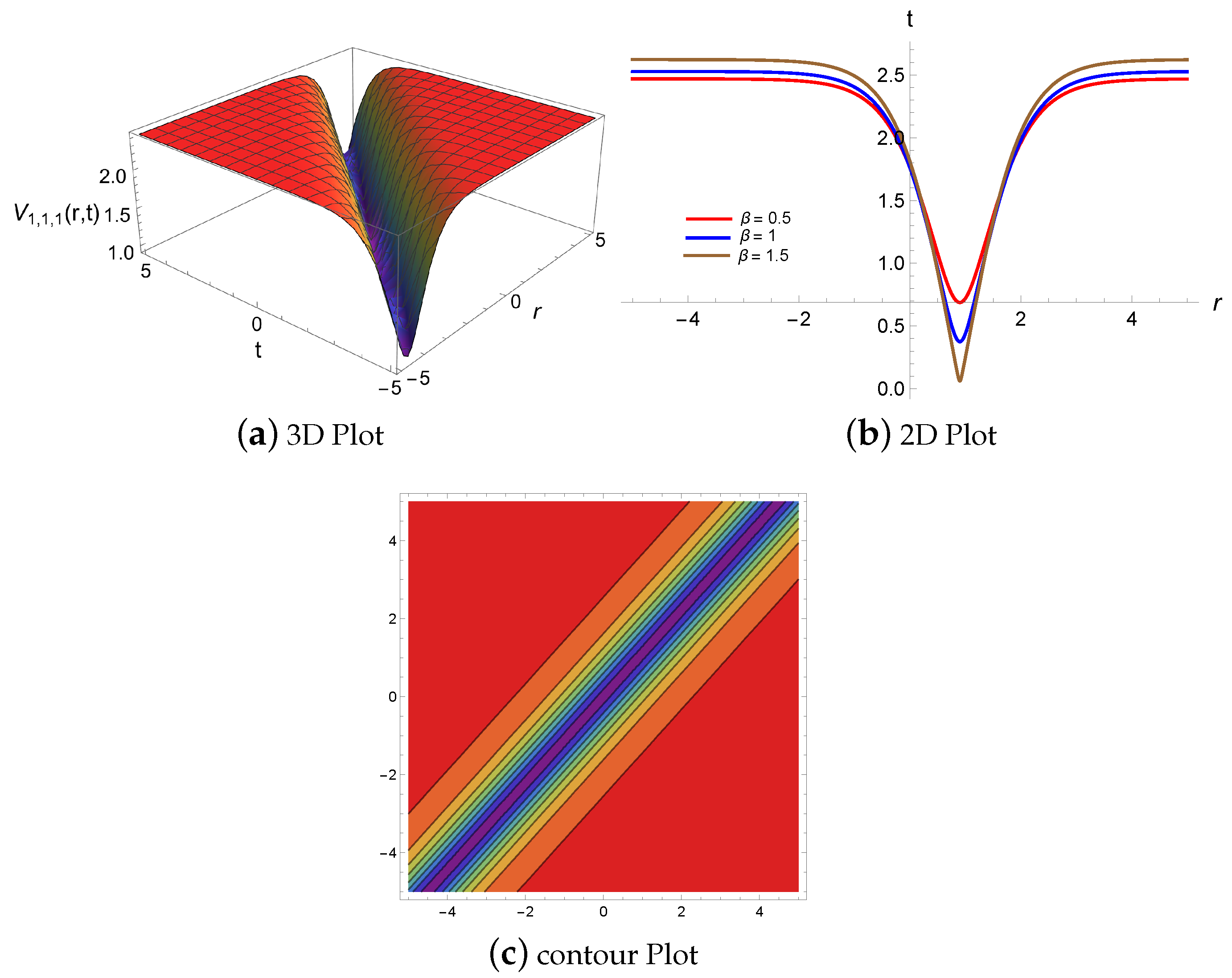
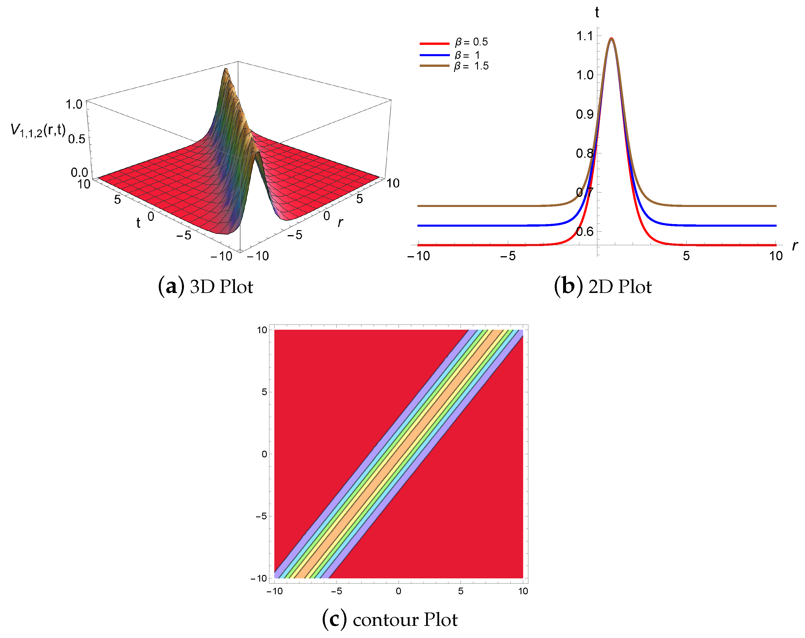
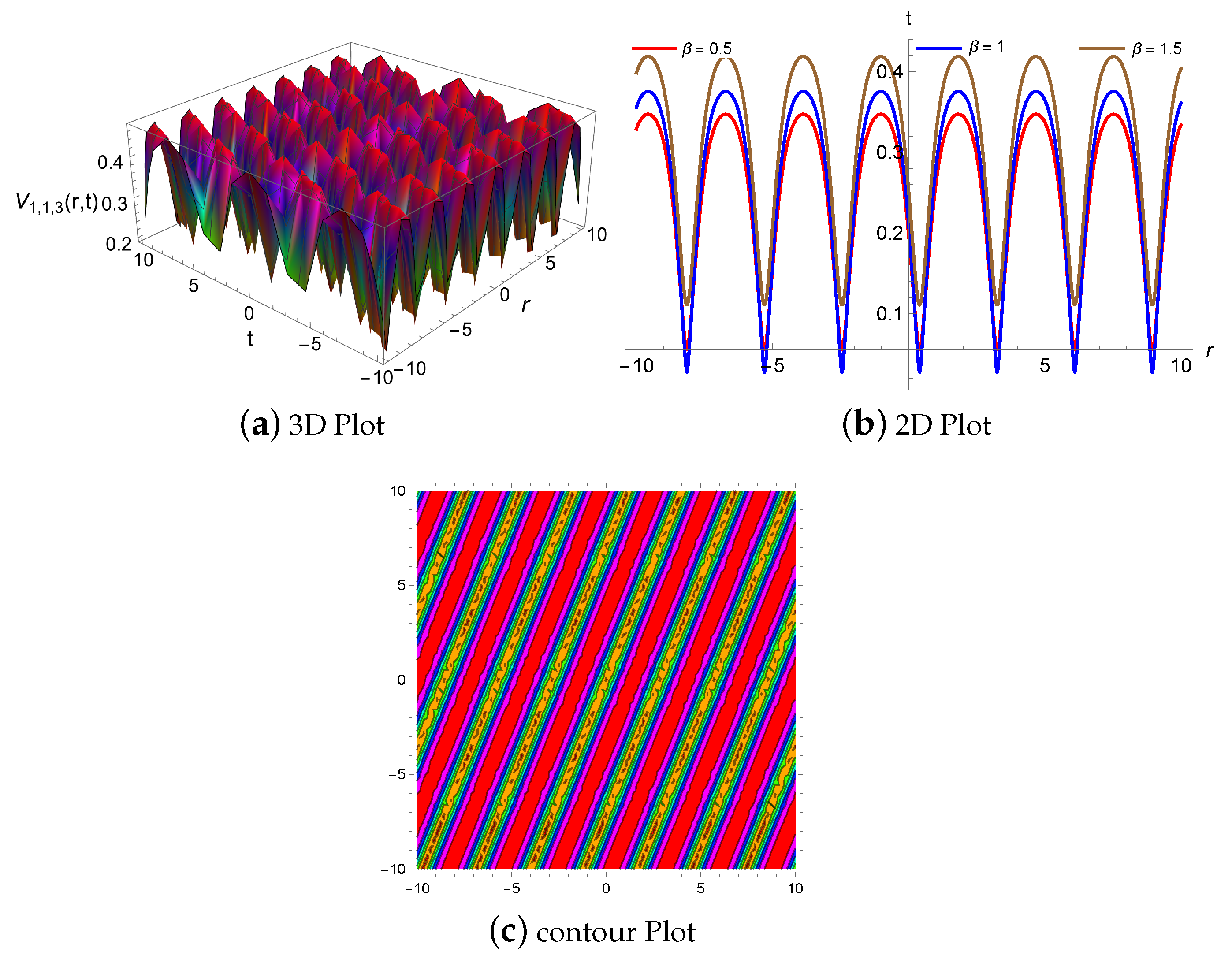
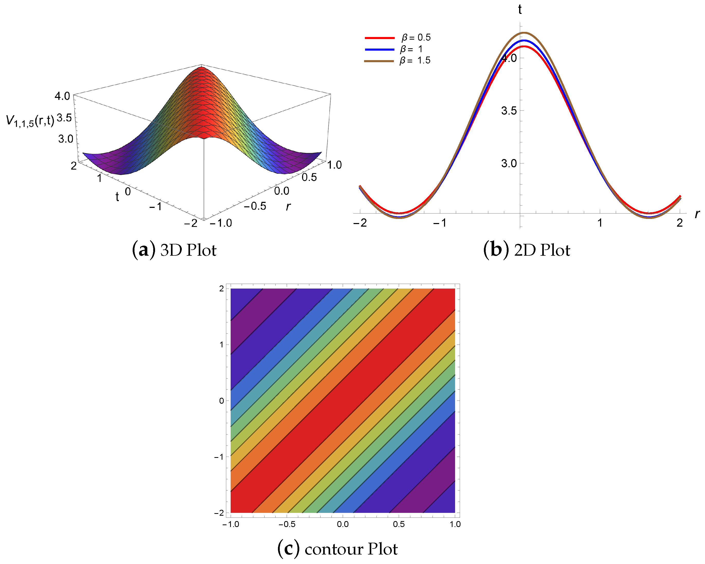
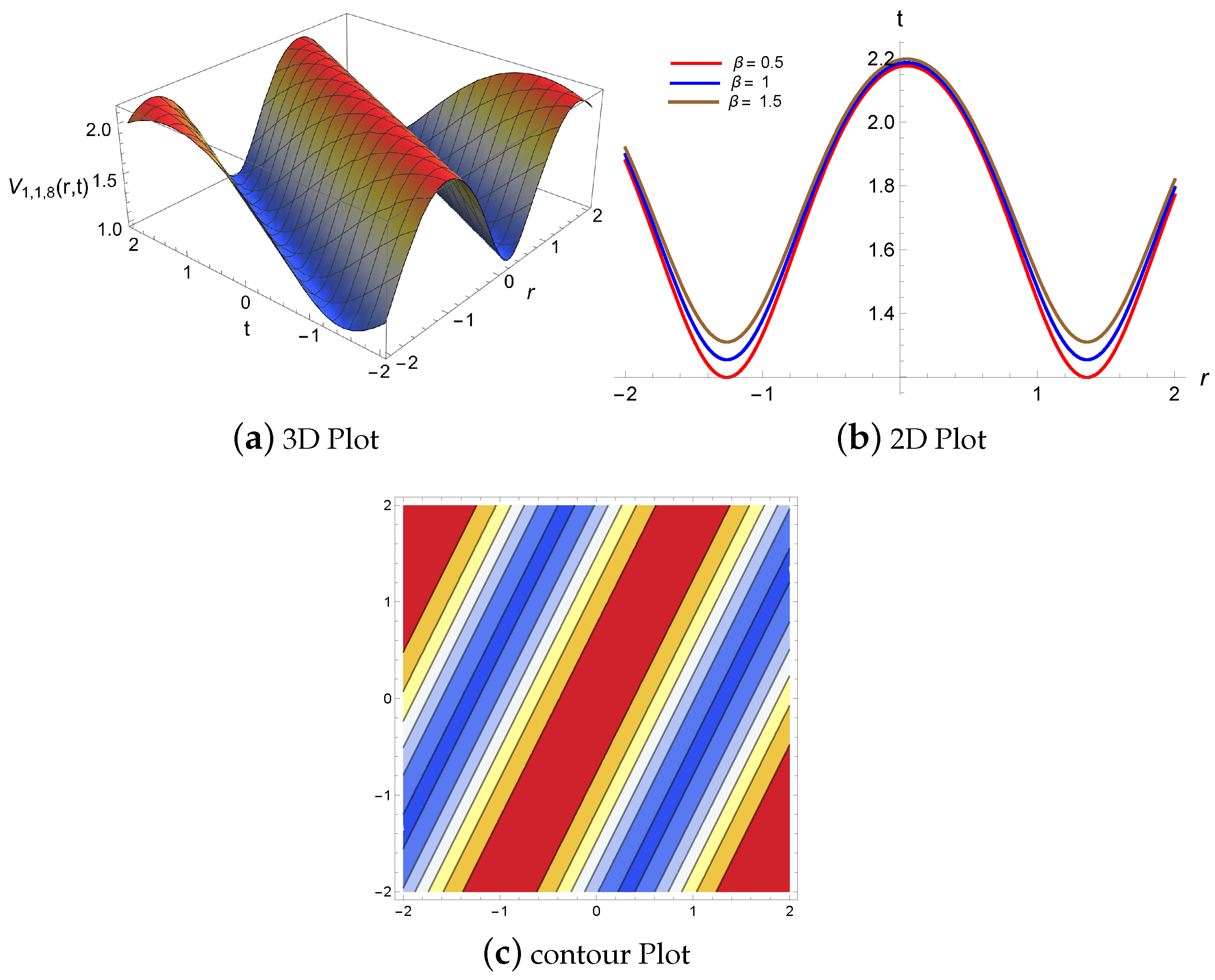
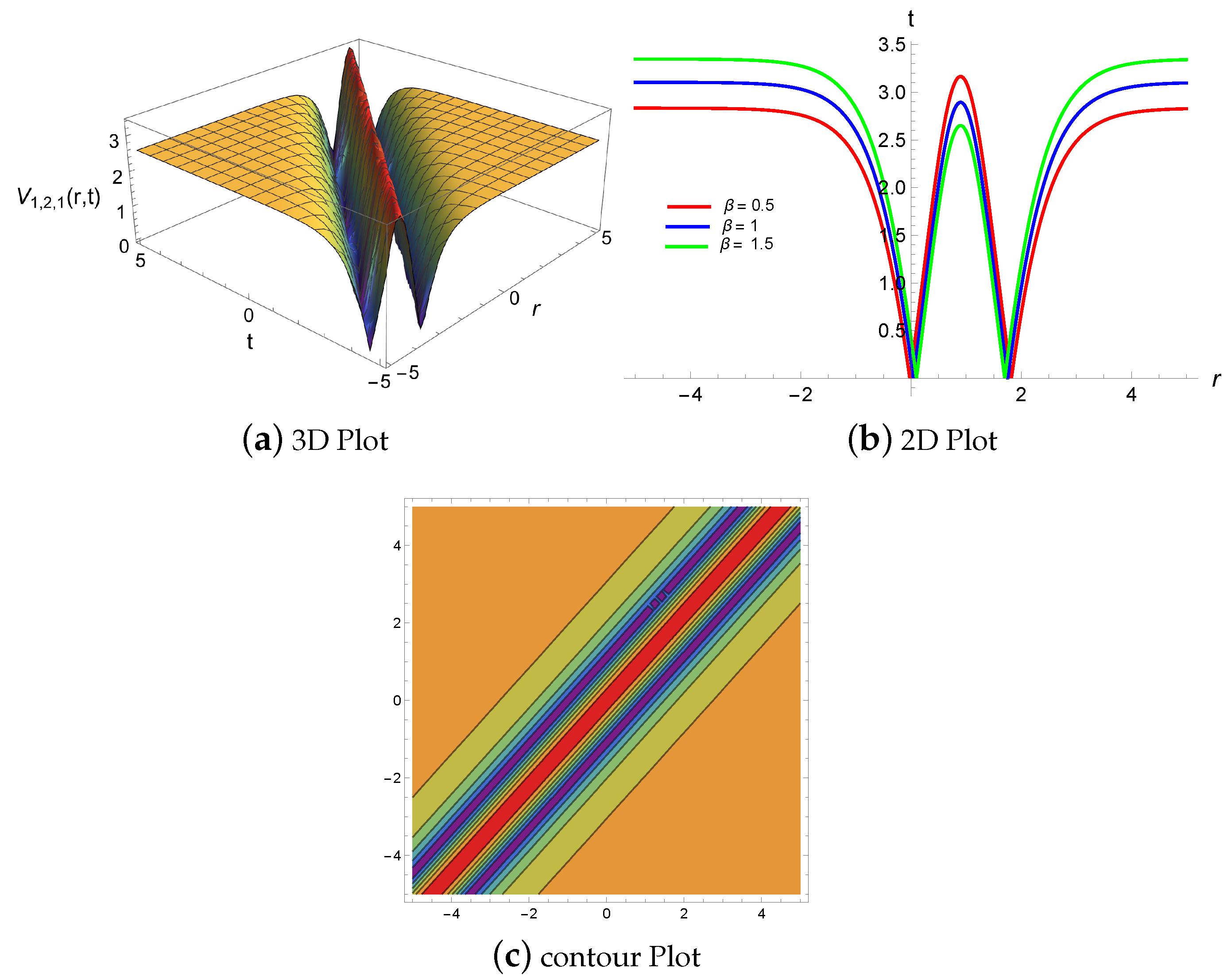
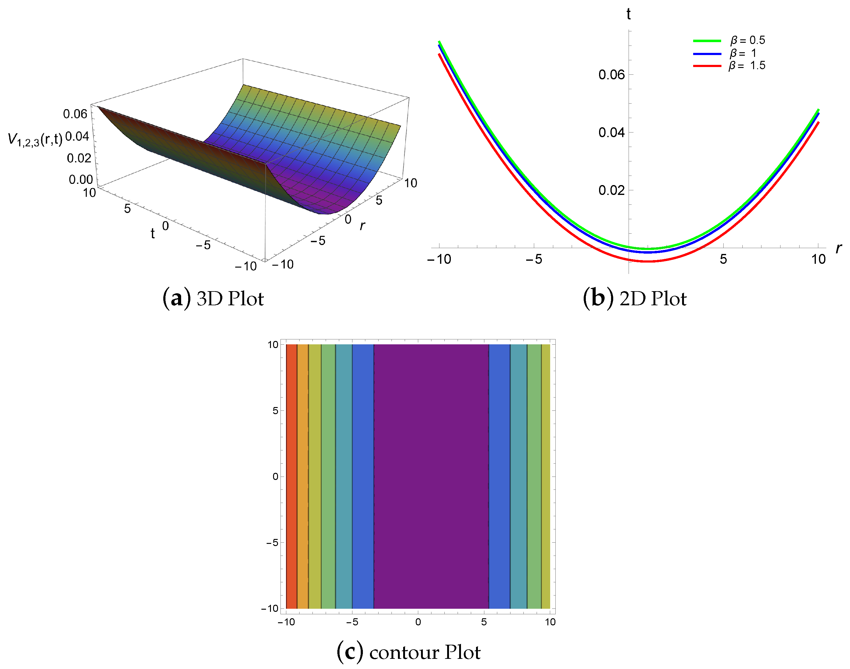
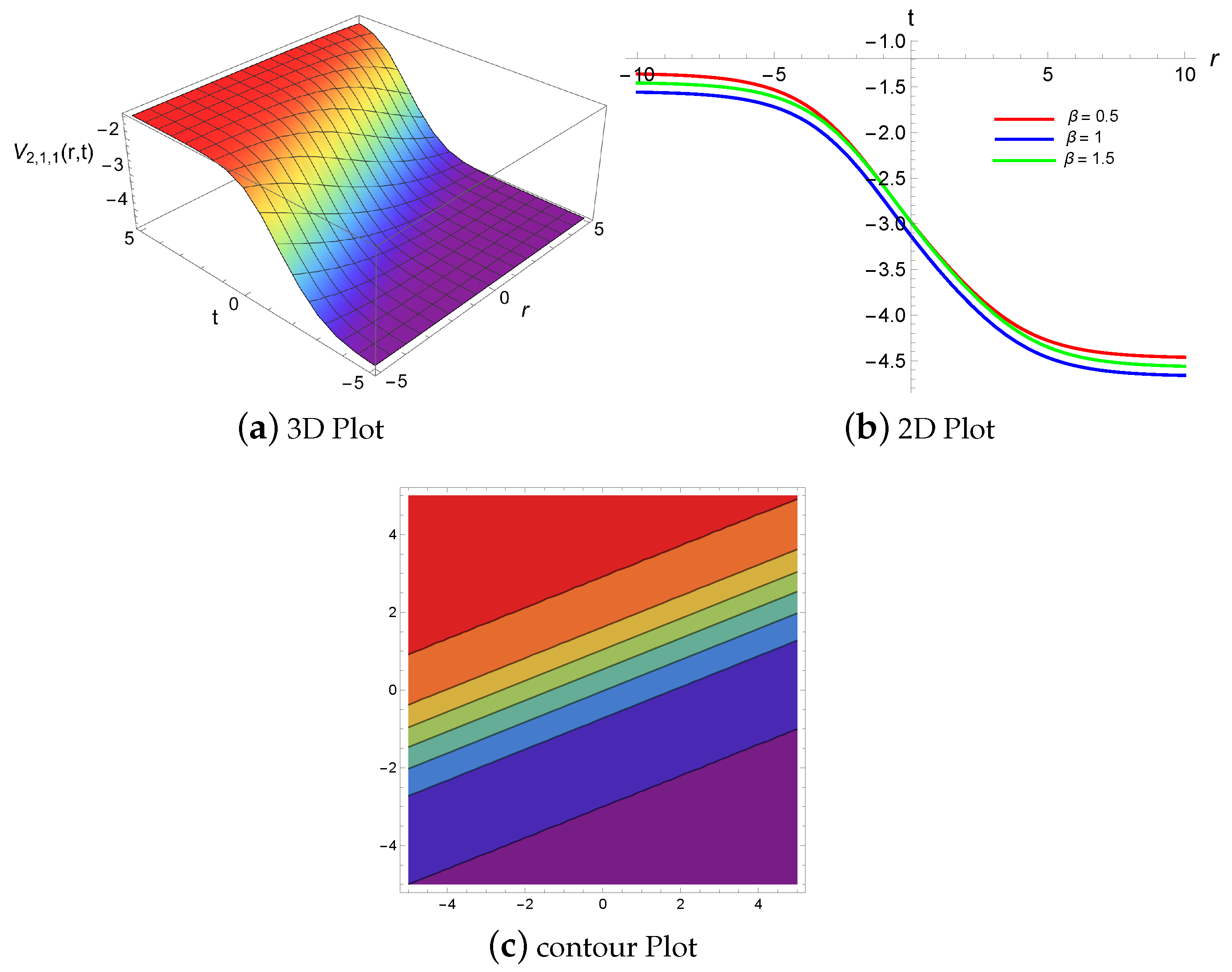
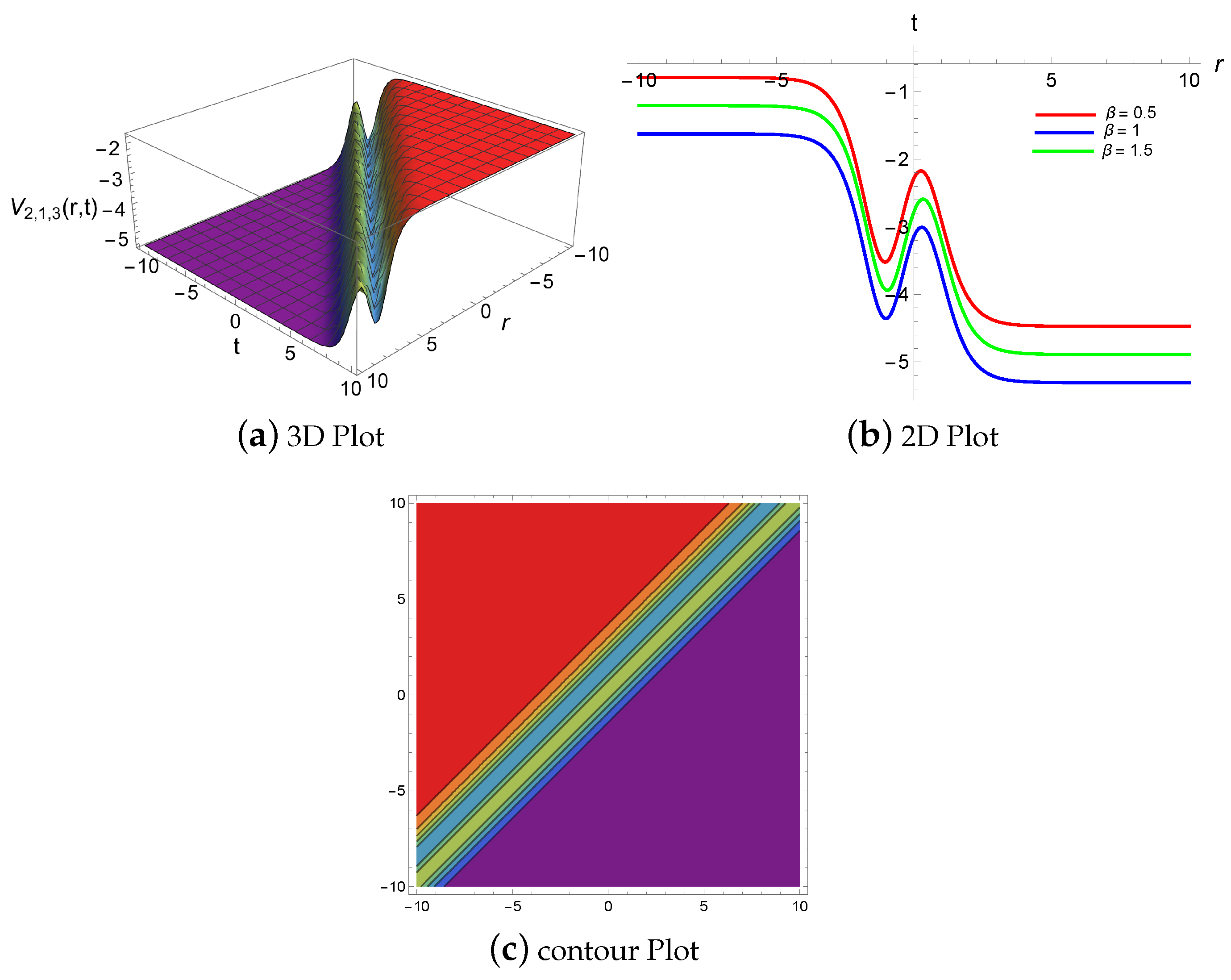
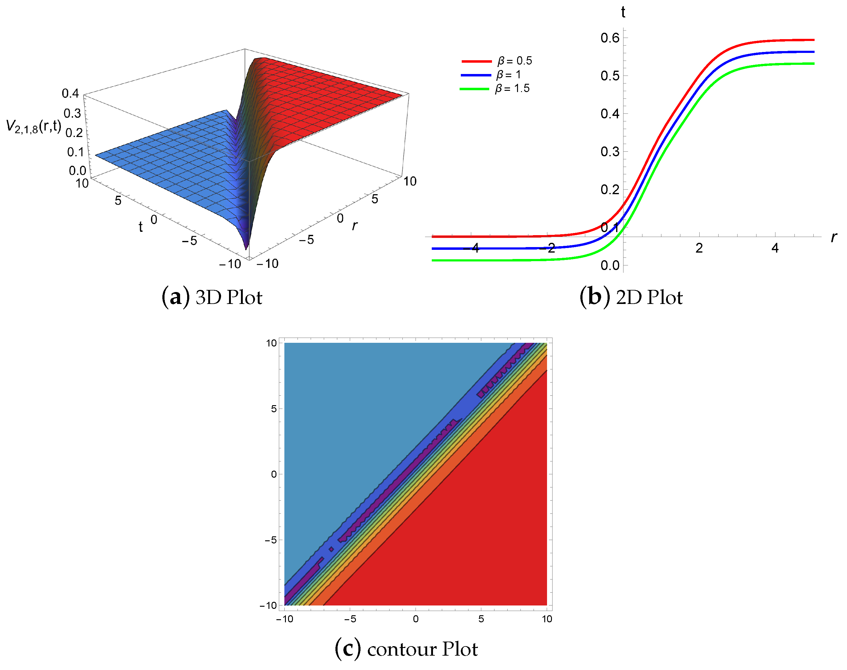
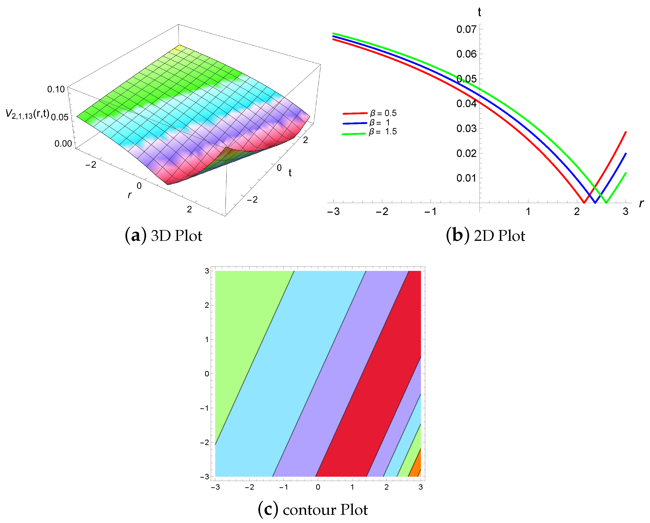
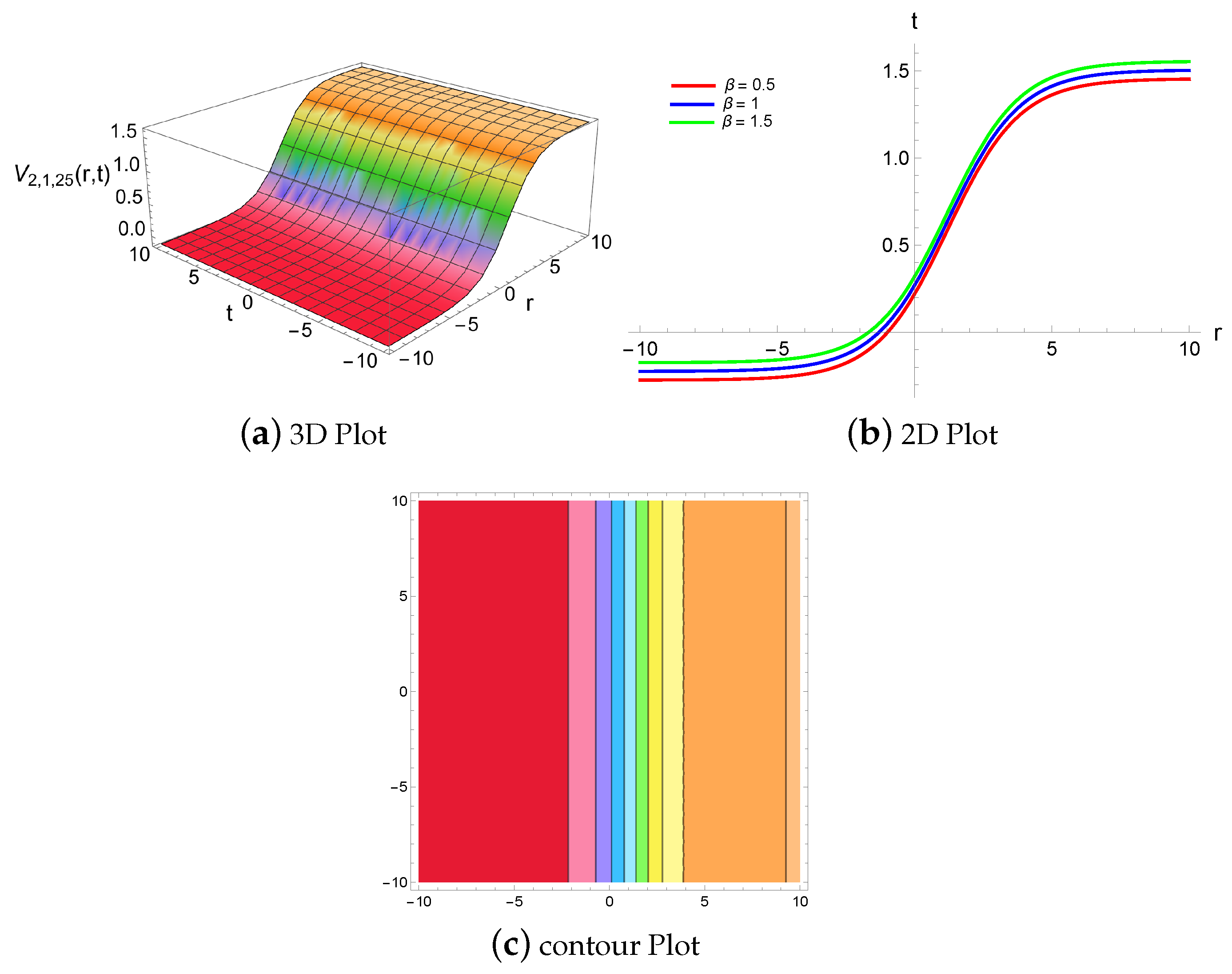
4.1. Physical Descriptions via Mapping Method

This portion shows the contour plots in addition to the 3D plots and corresponding 2D line graphs which are generated by using Mathematica 12. Specific waveforms such as dark, bright, bell-shaped, continuous periodic wave, W-shaped soliton and others can be found from generic exact solutions by changing the values of the free parameters. Each of these displays is influenced by the values of the indicated parameters in the exact solution that were recently found. Below is a list and discussion of the outcomes.

Figure 1 shows the 3D, 2D and contour plot representation of the result $V_{1,1,1}(\zeta )$ have been displayed for the values of the constants $\psi =0.9, a=1, \alpha =0.1, \beta =0.8, \lambda =0.1$ within the interval $-5\le r, t\le 5$. This representation is a dark soliton. The values of the wave velocity and constants satisfy the stability conditions. The results of the analysis are reliable. The values of the wave velocity and constants satisfy the stability conditions. The results of the analysis are reliable. For the values $\psi =0.8, a=1, \alpha =2, \beta =1, \lambda =-0.1$ of the parameters Figure 2 shows the 3D, 2D and contour plot representation of the result $V_{1,1,2}(\zeta )$ within the interval $-10\le r, t\le 10$, which is bright soliton. Figure 3 shows the continuous periodic wave soliton is the profile of result, $V_{1,1,3}(\zeta )$ for the value of the constant $\psi =1.6, a=1.5, \alpha =2, \beta =3, \lambda =0.09, b=1.2$, while the contour and 3D, 2D plots are displayed within the interval $-10\le r, t\le 10$. On the other hand, for the values $\psi =0.5, a=1, \alpha =0.1, \beta =0.9, \lambda =1, b=1.5$ of the parameters, the exact solution $V_{1,1,5}(\zeta )$ represents bell-shaped soliton in Figure 4. The contour 3D and 2D representations are revealed within the limit $-1\le r\le 1$ and $-2\le t\le 2$. Figure 5 displays the contour 3D and 2D representation of the obtained result $V_{1,1,8}(\zeta )$, which is a W-shaped soliton for the particular standards of the parameters $\psi =0.5, a=1, \alpha =0.1, \beta =0.9, \lambda =1, b=1.1$ within the range $-2\le r, t\le 2$. Conversely, Figure 6 shows the contour 3D and 2D depiction of the outcome which is displayed in the range $-5\le r, t\le 5$. The soliton $V_{1,2,1}(\zeta )$ is a W-shaped soliton for the values of the constants $\psi =0.9, a=1, \alpha =0.1, \beta =0.8, \lambda =0.1$. Figure 7 shows the exact solution $V_{1,2,3}(\zeta )$ for the constant values $\psi =0.01, a=0.01, \alpha =0.9, \beta =0.1, \lambda =0.09, b=1$, the contour, 3D and 2D representation of result $V_{1,2,3}(\zeta )$ have been presented with in the interval $-10\le r, t\le 10$. The result is dark soliton. For $\psi =1, a=0.5, \alpha =0.9, \beta =1, \gamma =0.2, b=1.5$, result $V_{1,2,6}(\zeta )$ delivers the continuous periodic wave soliton and portrayed in Figure 8 within the limit $-5\le r, t\le 5$.

4.2. Physical Descriptions via Generalized Riccati Equation Mapping Method

In this subsection, the primary goal of the study is to discuss the results obtained using the GREM method. The exact solutions are theoretically significant and physically meaningful. These exact solutions will be more advantageous if traveling wave solutions gain physical significance. Energy is transferred from one point to another primarily through traveling waves. The intensity of traveling waves, which are recognized for their capacity to transfer energy, can be associated with certain characteristics. Depending on the behavior of the parameters, the found exact solutions are classified as complex, real-valued, trigonometric, and hyperbolic functions. Below is a list and discussion of the outcomes.

Figure 9 shows that the exact solution $V_{2,1,1}(\zeta )$ gives the smooth kink soliton which rises from right to left. The 3D, 2D and contour representation of the achieved result $V_{2,1,1}(\zeta )$ are sketched for the specific standards of $\mu =1.9, \nu =1.5, \kappa =0.5, a=0.8, \psi =2, \beta =5, \alpha =2, \lambda =0.3$ within the limit $-5\le r, t\le 5$. Moreover, result $V_{2,1,3}(\zeta )$ also describes the rouge wave type soliton for the values $\mu =1.1, \nu =0.5, \kappa =0.5, a=1.9, \psi =1.9, \beta =1.2, \alpha =0.2, \lambda =0.3$. In the interval $-10\le r, t\le 10$, the physical representations are shown in Figure 10. A W-shaped soliton is the contexture of the exact solution $V_{2,1,7}(\zeta )$ with constant $\mu =3, \nu =0.15, \kappa =2.5, a=0.5, \psi =0.6, \beta =4, \alpha =2, \lambda =0.9, Q=1.2, P=1$. Figure 11 shows the 3D, 2D and contour representation of the outcome within the range of $-5\le r, t\le 5$. Figure 12 shows the exact solution $V_{2,1,8}(\zeta )$ for the constant values $\mu =2, \nu =0.85, \kappa =0.85, a=2, \psi =1.9, \beta =4, \alpha =2, \lambda =0.9$, the contour, 3D and 2D representation of result $V_{2,1,8}(\zeta )$ have been presented with in the interval $-10\le r, t\le 10$. The result is anti-peakon soliton. Once more, the 3D, 2D and contour representation of result $V_{2,1,13}(\zeta )$ are obtained and displayed in Figure 13 for the values of the constant $\mu =0.1, \nu =0.1, \kappa =0.5, a=0.11, \psi =0.05, \beta =10, \alpha =2, \lambda =3$ within the interval $-2\le r, t\le 2$. V-shaped soliton the exact solution is this representation. For the values $\mu =0.8, \nu =0.9, \kappa =1.2, a=0.04, \psi =0.05, \beta =1, \alpha =0.9, \lambda =2, Q=0.9, P=1$ of the parameters, Figure 14 shows the 3D, 2D and contour plot representation of the result $V_{2,1,18}(\zeta )$ within the interval $-5\le r, t\le 5$, which is flat wave soliton. For the values $\mu =1.5, \nu =1.2, \kappa =0, a=0.5, \psi =0.9, \beta =5, \alpha =2, \lambda =3, c=2$ of the parameters, Figure 15 shows the 3D, 2D and contour plot representation of the result $V_{2,1,25}(\zeta )$ within the interval $-10\le r, t\le 10$, which is kink wave soliton.

5. Conclusions

The exact solutions to the KG equation have been found in this research. One of the more fascinating problems in nuclear and high-energy physics has been figuring out the exact solutions to the KG equation. The KG equation has been widely used in relativistic quantum mechanics to characterize particle dynamics. Many efforts have been made recently to solve these relativistic wave equations for different potentials using various techniques. The exact solutions for the quadratic nonlinear KG model have been achieved by mapping and GREM methods. These often-used mathematical approaches have been recommended, permitting us to conduct complex and time-consuming algebraic computations. Both approaches have been successfully utilized while working with differential equations. It has been shown from the results that the mapping and GREM approaches are more accurate and need less computing power than the other approaches. With a wide range of free parameter values, the outcomes that have been obtained include the forms of trigonometric and hyperbolic functions for the GREM technique as well as hyperbolic and Jacobi elliptic functions via the mapping method. As a result, precise types of solitary waves such as dark, bright, periodic, W-shaped, smooth kink, rouge wave, anti-peakon, V-shaped, and flat soliton waves have been established. Figures have been created to show how the parametric variables, in particular, for various values, affect the soliton’s form using Mathematica capabilities. It needs to be emphasized that these methods are credible, reliable, and easy to use with different NLEEs. These results have been utilized in quantum field models and can contribute to a better understanding of the variety of events that arise in the many physical systems encompassed by the present framework.

References

1. Das, A.; Ghosh, P.; Chandra, S.; Raj, V. Electron acoustic peregrine breathers in a quantum plasma with 1-D temperature anisotropy. IEEE Trans. Plasma Sci. 2021, 50, 1598–1609. [Google Scholar]
2. Roshid, M.M.; Bairagi, T.; Rahman, M.M. Lump, interaction of lump and kink and solitonic solution of nonlinear evolution equation which describe incompressible viscoelastic Kelvin-Voigt fluid. Partial. Differ. Equations Appl. Math. 2022, 5, 100354. [Google Scholar]
3. Aljahdaly, N.H.; El-Tantawy, S.A.; Wazwaz, A.M.; Ashi, H.A. Adomian decomposition method for modelling the dissipative higher-order rogue waves in a superthermal collisional plasma. J. Taibah Univ. Sci. 2021, 15, 971–983. [Google Scholar]
4. Yao, S.W.; Zekavatm, S.M.; Rezazadeh, H.; Vahidi, J.; Ghaemi, M.B.; Inc, M. The solitary wave solutions to the Klein–Gordon-Zakharov equations by extended rational methods. Aip Adv. 2021, 11, 065218. [Google Scholar]
5. Malik, S.; Almusawa, H.; Kumar, S.; Wazwaz, A.M.; Osman, M.S. A (2 + 1)-dimensional Kadomtsev-Petviashvili equation with competing dispersion effect: Painlevé analysis, dynamical behavior and invariant solutions. Results Phys. 2021, 23, 104043. [Google Scholar]
6. Karjanto, N. Modeling Wave Packet Dynamics and Exploring Applications: A Comprehensive Guide to the Nonlinear Schrödinger Equation. Mathematics 2024, 12, 744. [Google Scholar] [CrossRef]
7. Kurt, A.; Tozar, A.; Tasbozan, O. Applying the new extended direct algebraic method to solve the equation of obliquely interacting waves in shallow waters. J. Ocean. Univ. China 2020, 19, 772–780. [Google Scholar]
8. Nadeem, M.; Iambor, L.F. The traveling wave solutions to a variant of the Boussinesq equation. Electron. J. Appl. Math. 2023, 1, 26–37. [Google Scholar]
9. Liu, S.H.; Tian, B.; Wang, M. Painlevé analysis, bilinear form, Bäcklund transformation, solitons, periodic waves and asymptotic properties for a generalized Calogero–Bogoyavlenskii–Konopelchenko–Schiff system in a fluid or plasma. Eur. Phys. J. Plus 2021, 136, 917. [Google Scholar]
10. Li, J.; Xu, C.; Lu, J. The exact solutions to the generalized (2 + 1)-dimensional nonlinear wave equation. Results Phys. 2024, 58, 107506. [Google Scholar]
11. Zhou, Q.; Huang, Z.; Sun, Y.; Triki, H.; Liu, W.; Biswas, A. Collision dynamics of three-solitons in an optical communication system with third-order dispersion and nonlinearity. Nonlinear Dyn. 2023, 111, 5757–5765. [Google Scholar]
12. Sun, Y.; Hu, Z.; Triki, H.; Mirzazadeh, M.; Liu, W.; Biswas, A.; Zhou, Q. Analytical study of three-soliton interactions with different phases in nonlinear optics. Nonlinear Dyn. 2023, 111, 18391–18400. [Google Scholar]
13. Alquran, M.; Alhami, R. Convex-periodic, kink-periodic, peakon-soliton and kink bidirectional wave-solutions to new established two-mode generalization of Cahn-Allen equation. Results Phys. 2022, 34, 105257. [Google Scholar]
14. Alquran, M.; Alhami, R. Analysis of lumps, single-stripe, breather-wave, and two-wave solutions to the generalized perturbed-KdV equation by means of Hirota’s bilinear method. Nonlinear Dyn. 2022, 109, 1985–1992. [Google Scholar]
15. Sarwar, A.; Gang, T.; Arshad, M.; Ahmed, I.; Ahmad, M.O. Abundant solitary wave solutions for space-time fractional unstable nonlinear Schrödinger equations and their applications. Ain Shams Eng. J. 2023, 14, 101839. [Google Scholar]
16. Abazari, R.; Jamshidzadeh, S. Exact solitary wave solutions of the complex Klein–Gordon equation. Opt. Int. J. Light Electron Opt. 2015, 126, 1970–1975. [Google Scholar]
17. Yang, Y.; Yang, X.; Wang, J.; Liu, J. The numerical solution of the time-fractional non-linear Klein–Gordon equation via spectral collocation method. Therm. Sci. 2019, 23 Part A, 1529–1537. [Google Scholar]
18. Alquran, M.; Dagher, A.; Al-Dolat, M. Exact Traveling Wave Solutions for the Celebrated Gardner Model and the Nonlinear Klein–Gordon System by Means of the Celebrated Unified Method. Int. J. Appl. Comput. Math. 2019, 5, 1–11. [Google Scholar]
19. Ma, W.X. Riemann-Hilbert problems and inverse scattering of nonlocal real reverse-spacetime matrix AKNS hierarchies. Phys. D Nonlinear Phenom. 2022, 430, 133078. [Google Scholar]
20. Alhojilan, Y.; Ahmed, H.M. Novel analytical solutions of stochastic Ginzburg-Landau equation driven by Wiener process via the improved modified extended tanh function method. Alex. Eng. J. 2023, 72, 269–274. [Google Scholar]
21. Chu, Y.M.; Fahim, M.R.A.; Kundu, P.R.; Islam, M.E.; Akbar, M.A.; Inc, M. Extension of the sine-Gordon expansion scheme and parametric effect analysis for higher-dimensional nonlinear evolution equations. J. King Saud Univ.-Sci. 2021, 33, 101515. [Google Scholar]
22. Rezazadeh, H.; Ullah, N.; Akinyemi, L.; Shah, A.; Mirhosseini-Alizamin, S.M.; Chu, Y.M.; Ahmad, H. Optical soliton solutions of the generalized non-autonomous nonlinear Schrödinger equations by the new Kudryashov’s method. Results Phys. 2021, 24, 104179. [Google Scholar]
23. Malik, S.; Hashemi, M.S.; Kumar, S.; Rezazadeh, H.; Mahmoud, W.; Osman, M.S. Application of new Kudryashov method to various nonlinear partial differential equations. Opt. Quantum Electron. 2023, 55, 8. [Google Scholar]
24. Raheel, M.; Zafar, A.; Nawaz, M.S.; Bekir, A.; Tariq, K.U. Exact soliton solutions to the time-fractional Kudryashov model via an efficient analytical approach. Pramana 2023, 97, 45. [Google Scholar]
25. Ouahid, L.; Abdou, M.A.; Kumar, S.; Owyed, S.; Ray, S.S. A plentiful supply of soliton solutions for DNA Peyrard-Bishop equation by means of a new auxiliary equation strategy. Int. J. Mod. Phys. B 2021, 35, 2150265. [Google Scholar]
26. Rehman, H.U.; Akber, R.; Wazwaz, A.M.; Alshehri, H.M.; Osman, M.S. Analysis of Brownian motion in stochastic Schrödinger wave equation using Sardar sub-equation method. Optik 2023, 289, 171305. [Google Scholar]
27. Cakicioglu, H.; Ozisik, M.; Secer, A.; Bayram, M. Optical soliton solutions of Schrödinger-Hirota equation with parabolic law nonlinearity via generalized Kudryashov algorithm. Opt. Quantum Electron. 2023, 55, 407. [Google Scholar]
28. Kabir, M.M.; Khajeh, A.; Abdi Aghdam, E.; Yousefi Koma, A. Modified Kudryashov method for finding exact solitary wave solutions of higher-order nonlinear equations. Math. Methods Appl. Sci. 2011, 34, 213–219. [Google Scholar]
29. Ebaid, A. Exact solutions for the generalized Klein–Gordon equation via a transformation and Exp-function method and comparison with Adomian’s method. J. Comput. Appl. Math. 2009, 223, 278–290. [Google Scholar]
30. Alaje, A.I.; Olayiwola, M.O.; Adedokun, K.A.; Adedeji, J.A.; Oladapo, A.O. Modified homotopy perturbation method and its application to analytical solitons of fractional-order Korteweg-de Vries equation. Beni-Suef Univ. J. Basic Appl. Sci. 2022, 11, 139. [Google Scholar]
31. Rizvi, S.T.R.; Seadawy, A.R.; Younis, M.; Ali, I.; Althobaiti, S.; Mahmoud, S.F. Soliton solutions, Painleve analysis and conservation laws for a nonlinear evolution equation. Results Phys. 2021, 23, 103999. [Google Scholar]
32. Hafez, M.G.; Alam, M.N.; Akbar, M.A. Exact traveling wave solutions to the Klein–Gordon equation using the novel (G’/G)-expansion method. Results Phys. 2014, 4, 177–184. [Google Scholar]
33. Billig, Y. Principal vertex operator representations for toroidal Lie algebras. J. Math. Phys. 1998, 39, 3844–3864. [Google Scholar]
34. Khalid, M.; Sultana, M.; Zaidi, F.; Arshad, U. Solving linear and nonlinear Klein–Gordon equations by new perturbation iteration transform method. Wms J. Appl. Eng. Math. 2016, 6, 115–125. [Google Scholar]
35. Sadiya, U.; Inc, M.; Arefin, M.A.; Uddin, M.H. Consistent travelling waves solutions to the non-linear time fractional Klein–Gordon and Sine-Gordon equations through extended tanh-function approach. J. Taibah Univ. Sci. 2022, 16, 594–607. [Google Scholar]
36. Alsisi, A. Analytical and numerical solutions to the Klein–Gordon model with cubic nonlinearity. Alex. Eng. J. 2024, 99, 31–37. [Google Scholar]
37. Bildik, N.; Deniz, S. New approximate solutions to the nonlinear Klein–Gordon equations using perturbation iteration techniques. Discret. Contin. Dyn. Syst.-S 2020, 13, 503. [Google Scholar]
38. Chowdhury, M.S.H.; Hashim, I. Application of homotopy-perturbation method to Klein–Gordon and sine-Gordon equations. Chaos Solitons Fractals 2009, 39, 1928–1935. [Google Scholar]
39. Mat Zin, S.; Abbas, M.; Abd Majid, A.; Md Ismail, A.I. A new trigonometric spline approach to numerical solution of generalized nonlinear Klien-Gordon equation. PLoS ONE 2014, 9, e95774. [Google Scholar]
40. Mat Zin, S.; Abd Majid, A.; Ismail, A.I.M.; Abbas, M. Application of Hybrid Cubic B-Spline Collocation Approach for Solving a Generalized Nonlinear Klien-Gordon Equation. Math. Probl. Eng. 2014, 2014, 108560. [Google Scholar]
41. Dehghan, M.; Ghesmati, A. Application of the dual reciprocity boundary integral equation technique to solve the nonlinear Klein–Gordon equation. Comput. Phys. Commun. 2010, 181, 1410–1418. [Google Scholar]
42. Zayed, E.M.; Alurrfi, K.A. Solitons and other solutions for two nonlinear Schrödinger equations using the new mapping method. Optik 2017, 144, 132–148. [Google Scholar]
43. Rehman, H.U.; Saleem, M.S.; Zubair, M.; Jafar, S.; Latif, I. Optical solitons with Biswas–Arshed model using mapping method. Optik 2019, 194, 163091. [Google Scholar]
44. Krishnan, E.V.; Al Gabshi, M.; Zhou, Q.; Khan, K.R.; Mahmood, M.F.; Xu, Y.; Biswas, A.; Belic, M. Solitons in optical metamaterials by mapping method. J. Optoelectron. Adv. Mater. 2015, 17, 511–516. [Google Scholar]
45. Rabie, W.B.; Khalil, T.A.; Badra, N.; Ahmed, H.M.; Mirzazadeh, M.; Hashemi, M.S. Soliton Solutions and Other Solutions to the (4 + 1)-Dimensional Davey–Stewartson–Kadomtsev–Petviashvili Equation using Modified Extended Mapping Method. Qual. Theory Dyn. Syst. 2024, 23, 87. [Google Scholar]
46. Rehman, H.U.; Seadawy, A.R.; Razzaq, S.; Rizvi, S.T. Optical fiber application of the Improved Generalized Riccati Equation Mapping method to the perturbed nonlinear Chen-Lee-Liu dynamical equation. Optik 2023, 290, 171309. [Google Scholar]
47. Ahmed, N.; Baber, M.Z.; Iqbal, M.S.; Annum, A.; Ali, S.M.; Ali, M.; Akgül, A.; El Din, S.M. Analytical study of reaction diffusion Lengyel–Epstein system by generalized Riccati equation mapping method. Sci. Rep. 2023, 13, 20033. [Google Scholar]
48. Hamad, I.S.; Ali, K.K. Investigation of Brownian motion in stochastic Schrödinger wave equation using the modified generalized Riccati equation mapping method. Opt. Quantum Electron. 2024, 56, 1–23. [Google Scholar]
49. Al-Amry, M.S.; Al-Shaoosh, M.M. The Generalized Riccati Equation Mapping for Solving (cmZKB) and (pZK) Equations. Univ. Aden J. Nat. Appl. Sci. 2019, 23, 201–210. [Google Scholar]
50. Hosseini, K.; Alizadeh, F.; Hinçal, E.; Kaymakamzade, B.; Dehingia, K.; Osman, M.S. A generalized nonlinear Schrödinger equation with logarithmic nonlinearity and its Gaussian solitary wave. Opt. Quantum Electron. 2024, 56, 929. [Google Scholar]
51. Agom, E.U.; Ogunfiditimi, F.O. Exact solution of nonlinear Klein–Gordon equations with quadratic nonlinearity by modified Adomian decomposition method. J. Math. Comput. Sci. 2018, 8, 484–493. [Google Scholar]
52. Roshid, M.M.; Karim, M.F.; Azad, A.K.; Rahman, M.M.; Sultana, T. New solitonic and rogue wave solutions of a Klein–Gordon equation with quadratic nonlinearity. Partial. Differ. Equations Appl. Math. 2021, 3, 100036. [Google Scholar]
Figure 1. The exact solution of V 1 , 1 , 1 ( ζ ) produces a dark soliton, when ψ = 0.9 ,   a = 1 ,   α = 0.1 ,   β = 0.8 ,   λ = 0.1 , (a) 3D plot at 5 r 5 and 5 t 5 (b) 2D plot for different values of β at t = 1 (c) contour plot of V 1 , 1 , 1 ( ζ ) .
Symmetry 16 01085 g001
Figure 2. The exact solution of V 1 , 1 , 2 ( ζ ) produces a bright soliton, when ψ = 0.8 ,   a = 1 ,   α = 2 ,   β = 1 ,   λ = 0.1 , (a) 3D plot at 10 r 10 and 10 t 10 (b) 2D plot for different values of β at t = 1 (c) contour plot of V 1 , 1 , 2 ( ζ ) .
Symmetry 16 01085 g002
Figure 3. The exact solution of V 1 , 1 , 3 ( ζ ) produces a continuous periodic wave soliton, when ψ = 1.6 ,   a = 1.5 ,   α = 2 ,   β = 3 ,   λ = 0.09 ,   b = 1.2 , (a) 3D plot at 10 r 10 and 10 t 10 (b) 2D plot for different values of β at t = 1 (c) contour plot of V 1 , 1 , 3 ( ζ ) .
Symmetry 16 01085 g003
Figure 4. The exact solution of V 1 , 1 , 5 ( ζ ) produces a bell-shaped soliton, when ψ = 0.5 ,   a = 1 ,   α = 0.1 ,   β = 0.9 ,   λ = 1 ,   b = 1.5 , (a) 3D plot at 1 r 1 and 2 t 2 (b) 2D plot for different values of β at t = 1 (c) contour plot of V 1 , 1 , 5 ( ζ ) .
Symmetry 16 01085 g004
Figure 5. The exact solution of V 1 , 1 , 8 ( ζ ) produces a W-shaped soliton, when ψ = 0.5 ,   a = 1 ,   α = 0.1 ,   β = 0.9 ,   λ = 1 ,   b = 1.1 ,   (a) 3D plot at 2 r 2 and 2 t 2 (b) 2D plot for different values of β at t = 1 (c) contour plot of V 1 , 1 , 8 ( ζ ) .
Symmetry 16 01085 g005
Figure 6. The exact solution of V 1 , 2 , 1 ( ζ ) produces a W-shaped soliton, when ψ = 0.9 ,   a = 1 ,   α = 0.1 ,   β = 0.8 ,   λ = 0.1 , (a) 3D plot at 5 r 5 and 5 t 5 (b) 2D plot for different values of β at t = 1 (c) contour plot of V 1 , 2 , 1 ( ζ ) .
Symmetry 16 01085 g006
Figure 7. The exact solution of V 1 , 2 , 3 ( ζ ) produces a dark soliton, when ψ = 0.01 ,   a = 0.01 ,   α = 0.9 ,   β = 0.1 ,   λ = 0.09 ,   b = 1 , (a) 3D plot 10 r 10 and 10 t 10 (b) 2D plot for different values of β at t = 1 (c) contour plot of V 1 , 2 , 3 ( ζ ) .
Symmetry 16 01085 g007
Figure 8. The exact solution of V 1 , 2 , 6 ( ζ ) produces a continuous periodic wave soliton, when ψ = 1 ,   a = 0.5 ,   α = 0.9 ,   β = 1 ,   γ = 0.2 ,   b = 1.5 , (a) 3D plot at 5 r 5 and 5 t 5 (b) 2D plot for different values of β at t = 1 (c) contour plot of V 1 , 2 , 6 ( ζ ) .
Symmetry 16 01085 g008
Figure 9. The exact solution of V 2 , 1 , 1 ( ζ ) produces a smooth kink wave soliton, when μ = 1.9 ,   ν = 1.5 ,   κ = 0.5 ,   a = 0.8 ,   ψ = 2 ,   β = 5 ,   α = 2 ,   λ = 0.3 (a) 3D plot at 5 r 5 and 5 t 5 (b) 2D plot for different values of β at t = 1 (c) contour plot of V 2 , 1 , 1 ( ζ ) .
Symmetry 16 01085 g009
Figure 10. The exact solution of V 2 , 1 , 3 ( ζ ) produces a rouge wave soliton, when μ = 1.1 ,   ν = 0.5 ,   κ = 0.5 ,   a = 1.9 ,   ψ = 1.9 ,   β = 1.2 ,   α = 0.2 ,   λ = 0.3 (a) 3D plot at 10 r 10 and 10 t 10 (b) 2D plot for different values of β at t = 1 (c) contour plot of V 2 , 1 , 3 ( ζ ) .
Symmetry 16 01085 g010
Figure 11. The exact solution of V 2 , 1 , 7 ( ζ ) produces a W-shaped soliton, when μ = 3 ,   ν = 0.15 ,   κ = 2.5 ,   a = 0.5 ,   ψ = 0.6 ,   β = 4 ,   α = 2 ,   λ = 0.9 ,   Q = 1.2 ,   P = 1 (a) 3D plot at 5 r 5 and 5 t 5 (b) 2D plot for different values of β at t = 1 (c) contour plot of V 2 , 1 , 7 ( ζ ) .
Symmetry 16 01085 g011
Figure 12. The exact solution of V 2 , 1 , 8 ( ζ ) produces anti-peakon soliton, when μ = 2 ,   ν = 0.85 ,   κ = 0.85 ,   a = 2 ,   ψ = 1.9 ,   β = 4 ,   α = 2 ,   λ = 0.9 (a) 3D plot at 10 r 10 and 10 t 10 (b) 2D plot for different values of β at t = 1 (c) contour plot of V 2 , 1 , 8 ( ζ ) .
Symmetry 16 01085 g012
Figure 13. The exact solution of V 2 , 1 , 13 ( ζ ) produces a V-shaped soliton, when μ = 0.1 ,   ν = 0.1 ,   κ = 0.5 ,   a = 0.11 ,   ψ = 0.05 ,   β = 10 ,   α = 2 ,   λ = 3 (a) 3D plot at 2 r 2 and 2 t 2 (b) 2D plot for different values of β at t = 1 (c) contour plot of V 2 , 1 , 13 ( ζ ) .
Symmetry 16 01085 g013
Figure 14. The exact solution of V 2 , 1 , 18 ( ζ ) produces a flat wave soliton, when μ = 0.8 ,   ν = 0.9 ,   κ = 1.2 ,   a = 0.04 ,   ψ = 0.05 ,   β = 1 ,   α = 0.9 ,   λ = 2 ,   Q = 0.9 ,   P = 1 (a) 3D plot at 5 r 5 and 5 t 5 (b) 2D plot for different values of β at t = 1 (c) contour plot of V 2 , 1 , 18 ( ζ ) .
Symmetry 16 01085 g014
Figure 15. The exact solution of V 2 , 1 , 25 ( ζ ) produces a kink wave soliton, when μ = 1.5 ,   ν = 1.2 ,   κ = 0 ,   a = 0.5 ,   ψ = 0.9 ,   β = 5 ,   α = 2 ,   λ = 3 ,   c = 2 (a) 3D plot at 10 r 10 and 10 t 10 (b) 2D plot for different values of β at t = 1 (c) contour plot of V 2 , 1 , 25 ( ζ ) .
Symmetry 16 01085 g015
Disclaimer/Publisher’s Note: The statements, opinions and data contained in all publications are solely those of the individual author(s) and contributor(s) and not of MDPI and/or the editor(s). MDPI and/or the editor(s) disclaim responsibility for any injury to people or property resulting from any ideas, methods, instructions or products referred to in the content.