Generating Chaos in Dynamical Systems: Applications, Symmetry Results, and Stimulating Examples

Abstract

In this paper, we present a new class of extended oscillators in light of chaos theory. It is based on dynamical complex systems built on the concept of self-describing with a stopping criterion process. We offer an effective studying approach with a specific focus on learning, provoking students’ thinking through the triad of enigmatics–creativity–acmeology. Dynamic processes are the basis of mathematical modeling; thus, we can reach the goal of the above-mentioned triad by the proposed differential systems. The results we derive strongly confirm the presence of symmetry in the outcomes of the proposed models. We suggest a stochastic approach to structuring the proposed dynamical systems by modeling the coefficients that drive them by some discrete probability distribution that exhibits symmetry or asymmetry. We propose specific tools for researching the behavior of these systems.

1. Introduction

Chaos theory models dynamical complex systems built on the concept of self-describing with a stopping criterion process. Our idea in this direction is to realize the goal of effective training with a specific focus on applications in entertainment, which motivates and stimulates learners towards the triad of enigmatics–creativity–acmeology. Dynamic processes are the basis of mathematical modeling, and in this context, fun, if implemented in the daily learning activity, can reach the goal of the above-mentioned triad.

Challenges in this context are the interesting nuances of mathematical modeling in the main tools of chaos theory and, in modern technological society, the so-called computer mathematical modeling. It can be argued that it is the basis of optimization processes in all areas of scientific knowledge.

The attractiveness of trajectories in the attractor spectrum, regardless of the scientific field in which they are used, with their dynamics implemented with mathematical models (especially when using computer technologies) leads to provoking abilities in learners to see the properties and relationships in the modeled object and to develop their structural thinking.

The reader can find a comprehensive study on this topic in the magnificent monograph [1].

In this article, we present a new class of hypothetical oscillators. We also demonstrate some specialized modules for investigating their dynamics. The proper choice of the parameters that drive these dynamical systems is of outstanding importance. This motivates us to consider several examples that illustrate the possible arising behaviors. Sometimes, the dynamical systems that describe specific real-life phenomena exhibit forward as well as backward behavior. This motivates us to consider illustrations positioned on the real line (positive and negative). Such an example arises in finance: the primary markets are driven by forward dynamics, whereas the market of the derivatives (options, features, swaps, etc.) is rather considered to be driven by backward dynamics. In addition, we consider some models under the assumption that the parameters are generated by some discrete probability distribution. Thus, we introduce an appropriate mass for the different terms in the proposed models. As a result, the characteristic function of the chosen distribution arises in the oscillator’s dynamics.

2. A Modified Classic Model for Training on the Subject of Chaos Generation

The first-order Melnikov function for perturbed planar analytic systems of the form

$${\mathbf{x}}^{\prime }=\mathbf{f}\left(\mathbf{x}\right)+ϵ\mathbf{g}(\mathbf{x},ϵ,\mu )$$

(1)

with $\mathbf{x}\in R^2,\mu \in R^m$, is discussed in detail in [2,3,4].

For $ϵ=0$, system (1) has a one-parametric family of alternate orbits ${\mathrm{\Gamma }}_{\alpha }:x={\gamma }_{\alpha }\left(t\right),T_{\alpha }>t\ge 0$ of period $T_{\alpha }$ with parameter $\alpha \in I\subset R$ being equal to the arc length together with an arc $\mathrm{\sum }$ normal to the family ${\mathrm{\Gamma }}_{\alpha }$.

It is known that the Melnikov function for dynamics (1) is given by

$$M(\alpha ,\mu )={\int }_0^{T_{\alpha }}{e}^{-{\int }_0^t\nabla .f\left({\gamma }_{\alpha }\left(s\right)\right)ds}f\left({\gamma }_{\alpha }\left(t\right)\right)\wedge g({\gamma }_{\alpha }\left(t\right),0,\mu )dt,$$

where $T_{\alpha }$ is the period of ${\gamma }_{\alpha }\left(t\right)$ for $\alpha \in I$.

For the purpose of training on the topic of generating chaos in dynamical systems, it is appropriate to consider the following modification that has become a classic example:

$$\left\{\begin{array}{ccc}{\displaystyle \frac{dx}{dt}}\hfill & =& y+ϵ{\displaystyle \sum _{i=1}^n}{\mu }_i{x}^{2i-1}\hfill \\ {\displaystyle \frac{dy}{dt}}\hfill & =& x-x^3\hfill \\ \hfill & & n=2 ,3, \dots ,\hfill \end{array}\right.$$

(2)

with parameter $\mu =({\mu }_1, {\mu }_2, \dots , {\mu }_n)$.

2.1. The Case Where $n=2$ (Known Result)

Here, we will follow a part of the exposition in Perko’s monograph [3].

The one-parameter family of periodic orbits ${\gamma }_{\alpha }\left(t\right)=\{x_{\alpha }\left(t\right),y_{\alpha }\left(t\right)\}$ can be represented in terms of Jacoby elliptic functions [5] as (see Figure 1)

$$\begin{array}{c}{x}_0\left(t\right)={\displaystyle \frac{\sqrt{2}}{\sqrt{2-{\alpha }^2}}}dn\left({\displaystyle \frac{t}{\sqrt{2-{\alpha }^2}}},\alpha \right)\hfill \\ y_0\left(t\right)=-{\displaystyle \frac{\sqrt{2}{\alpha }^2}{2-{\alpha }^2}}sn\left({\displaystyle \frac{t}{\sqrt{2-{\alpha }^2}}},\alpha \right)cn\left({\displaystyle \frac{t}{\sqrt{2-{\alpha }^2}}},\alpha \right)\hfill \end{array}$$

(3)

for $0\le t\le T_{\alpha }$, where the period ${ }_{\alpha }$ takes the form $T_{\alpha }=2K\left(\alpha \right)\sqrt{2-{\alpha }^2}$ and $\alpha \in (0,1)$. $K\left(\alpha \right)$ is the complete elliptic integral of the first kind.

The parameter $\alpha$ is related to the distance along the x-axis by $x^2={\displaystyle \frac{2}{2-{\alpha }^2}}$. Evidently, ${\displaystyle \frac{\partial x}{\partial \alpha }}>0$ for $\alpha \in (0,1)$ or equivalently for $x\in (1,\sqrt{2})$. For $ϵ=0$, the system is Hamiltonian, i.e., $\nabla .f\left(x\right)=0$. Therefore, the Melnikov function together with the periodic orbit ${\gamma }_{\alpha }\left(t\right)$ is represented by

$$\begin{array}{ccc}M(\alpha ,\mu )\hfill & =& {\int }_0^{T_{\alpha }}f\left({\gamma }_{\alpha }\left(t\right)\right)\wedge g({\gamma }_{\alpha }\left(t\right),0,\mu )dt\hfill \\ & =& {\int }_0^{T_{\alpha }}\left({\mu }_2{x}_{\alpha }^6\left(t\right)+({\mu }_1-{\mu }_2)x_{\alpha }^4\left(t\right)-{\mu }_1{x}_{\alpha }^2\left(t\right)\right)dt\hfill \end{array}$$

Thus, refs. [2,3] lead to

$$\begin{array}{ccc}M(\alpha ,\mu )\hfill & =& {\displaystyle \frac{4}{{(2-{\alpha }^2)}^{\frac{5}{2}}}}\left({\displaystyle \frac{4{\mu }_2}{15}}\left(4(2-{\alpha }^2)({\alpha }^2-1)K\left(\alpha \right)+(8{\alpha }^4-23{\alpha }^2+23)E\left(\alpha \right)\right)\right.\hfill \\ & & -{\displaystyle \frac{2{\mu }_2}{3}}(2-{\alpha }^2)\left(({\alpha }^2-1)K\left(\alpha \right)+2(2-{\alpha }^2)E\left(\alpha \right)\right)\hfill \\ & & +{\displaystyle \frac{{\mu }_{1}2(2-{\alpha }^2)}{3}}\left(({\alpha }^2-1)K\left(\alpha \right)+2(2-{\alpha }^2)E\left(\alpha \right)\right)\hfill \\ & & \left.-{\mu }_1(4-4{\alpha }^2+{\alpha }^4)E\left(\alpha \right)\right),\hfill \end{array}$$

where $\mu =({\mu }_1,{\mu }_2)$, and $E\left(\alpha \right)$ and $K\left(\alpha \right)$ are the complete elliptic integrals of the first and second kind, respectively.

The function $M(\alpha ,\mu )$ measures the leading order distance between the stable and unstable manifolds and can be used to determine where the stable and unstable manifolds cross transversely.

It is known that for ${\mu }_2>0$ and $ϵ>0$, the system in this example has, above a critical threshold, a Hopf bifurcation at the critical point $\pm (1,-ϵ({\mu }_1+{\mu }_2))$ at ${\displaystyle \frac{{\mu }_1}{{\mu }_2}}=-3$.

For given ${\mu }_1=-2.9$, ${\mu }_2=1$, and $ϵ=0.085$, the simulations on system (2) for $n=2$, $x_0=0.3$, and $y_0=0.2$ are depicted in Figure 2.

The Melnikov function for $n=2$, ${\mu }_1=-2.9$, ${\mu }_2=1$, and $0.01<\alpha <0.99$ is depicted in Figure 3.

2.2. The Case Where $n=3$ (Unpublished Result)

The Melnikov function together with the periodic orbit ${\gamma }_{\alpha }\left(t\right)$ is represented by

$$\begin{array}{ccc}M(\alpha ,\mu )\hfill & =& {\int }_0^{T_{\alpha }}f\left({\gamma }_{\alpha }\left(t\right)\right)\wedge g({\gamma }_{\alpha }\left(t\right),0,\mu )dt\hfill \\ & =& {\int }_0^{T_{\alpha }}\left({\mu }_3{x}_{\alpha }^8\left(t\right)+({\mu }_2-{\mu }_3)x_{\alpha }^6\left(t\right)+({\mu }_1-{\mu }_2)x_{\alpha }^4\left(t\right)-{\mu }_1{x}_{\alpha }^2\left(t\right)\right)dt.\hfill \end{array}$$

By letting $u={\displaystyle \frac{t}{\sqrt{2-{\alpha }^2}}}$, we find that

$$\begin{array}{ccc}M(\alpha ,\mu )\hfill & =& {\displaystyle \frac{1}{{(2-{\alpha }^2)}^{\frac{7}{2}}}}{\int }_0^{4K\left(\alpha \right)}\left(8{\mu }_{3}d{n}^8\left(u\right)+4({\mu }_2-{\mu }_3)(2-{\alpha }^2)d{n}^6\left(u\right)\right.\hfill \\ & & \left.+2({\mu }_1-{\mu }_2){(2-{\alpha }^2)}^{2}d{n}^4\left(u\right)-{\mu }_1{(2-{\alpha }^2)}^{3}d{n}^2\left(u\right)\right)du.\hfill \end{array}$$

By using the formulae for the integrals of even powers of $dn\left(u\right)$ (see [5]), we find that

$$\begin{array}{ccc}M(\alpha ,\mu )\hfill & =& {\displaystyle \frac{1}{{(2-{\alpha }^2)}^{\frac{7}{2}}}}\left({\displaystyle \frac{8{\mu }_3}{105}}(-32(-2+{\alpha }^2)(11+{\alpha }^2(-11+6{\alpha }^2))E\left(\alpha \right)\right.\hfill \\ & & +4(-1+{\alpha }^2)(71+{\alpha }^2(-71+24{\alpha }^2))K\left(\alpha \right))\hfill \\ & & +{\displaystyle \frac{4({\mu }_2-{\mu }_3)(2-{\alpha }^2)}{15}}((23+{\alpha }^2(8{\alpha }^2-23))E\left(\alpha \right)-4({\alpha }^2-2)({\alpha }^2-1)K\left(\alpha \right))\hfill \\ & & +{\displaystyle \frac{2({\mu }_1-{\mu }_2){(2-{\alpha }^2)}^2}{3}}(-8({\alpha }^2-2)E\left(\alpha \right)+4({\alpha }^2-1)K\left(\alpha \right))\hfill \\ & & \left.-4{\mu }_1{(2-{\alpha }^2)}^{3}E\left(\alpha \right)\right),\hfill \end{array}$$

where $\mu =({\mu }_1,{\mu }_2,{\mu }_3)$.

For given ${\mu }_1=0.5$, ${\mu }_2=0.84$, ${\mu }_3=0.59$, and $ϵ=0.075$, the simulations on system (2) for $n=3$, $x_0=0.3$, and $y_0=0.2$ are depicted in Figure 4.

A detailed study of the nonlinear equation $M(\alpha ,\mu )=0$ is beyond the scope of the present study.

For example, the Melnikov function for $n=3$, $0.01<\alpha <0.99$ and fixed ${\mu }_1=-5.5$, ${\mu }_2=1.84$, and ${\mu }_3=1.59$ (A), is depicted in Figure 5. For ${\mu }_1=-0.1$, ${\mu }_2=-0.08$, and ${\mu }_3=-0.1$ (B), see Figure 6. For ${\mu }_1=1.91$, ${\mu }_2=0.19$, and ${\mu }_3=-0.1$ (C), see Figure 7.

Challenges for Learners

Task: 1. Try to obtain the Melnikov function for $n\ge 4$ in an explicit form. 2. Run simulations with this model, for example, with fixed $n=4;{\mu }_1=0.5;{\mu }_2=0.89;$${\mu }_3=-0.59;$${\mu }_4=0.08;ϵ=0.0075$. With a correct solution, you should obtain an image similar to that illustrated in Figure 8. 3. Make inferences about the sensitivity of the model as a function of its parameters.

2.3. Dynamics Controlled by a Probability Distribution

Suppose that the coefficients ${\mu }_1$, ${\mu }_2$, …, ${\mu }_n$ that drive dynamics (2) are positive and that their sum is one. Thus, we can view them as the probabilities of some discrete finite distribution. In fact, the important condition is the positiveness of ${\mu }_1$, ${\mu }_2$, …, ${\mu }_n$. Indeed, if $\mu ={\sum }_{i=1}^n{\mu }_i$, ${\overline{\mu }}_i={\displaystyle \frac{{\mu }_i}{\mu }}$, and $\overline{ϵ}=\mu ϵ$, then the other required condition is satisfied. Let us denote by $\xi$ a random variable exhibiting such distribution, i.e., its domain is the set $\left\{0,1,2,\dots ,n-1\right\}$ and $\mathbb{P}\left(\xi =i\right)={\mu }_i$. We will use the symbol $\mathbb{E}$ for the expectation through this law. Also, we denote by $\varphi \left(·\right)$ the moment-generating function (MGF) of $\xi$. Under these considerations, we can rewrite dynamics (2) as

$$\begin{array}{cc}\hfill {\displaystyle \frac{dx}{dt}}& =y+ϵ\sum _{i=1}^n{\mu }_i{x}^{2i-1}\hfill \\ \hfill & =y+ϵx\sum _{i=0}^{n-1}{\mu }_i{e}^{2i ln\left|x\right|}\hfill \\ \hfill & =y+ϵx\mathbb{E}\left[e^{2\xi ln\left|x\right|}\right]\hfill \\ \hfill & =y+ϵx\varphi \left(2ln\left|x\right|\right).\hfill \end{array}$$

(4)

Let us consider the examples provided in Section 4 of [6]; we assume that the random variable $\xi$ is distributed via the discrete uniform, binomial, $\beta$-binomial, or hypergeometric law. Thus, the values of ${\mu }_i$, $i=0,1,\dots ,n-1$, are

$$\begin{array}{cc}\hfill {\mu }_i^{\mathrm{uniform}}& ={\displaystyle \frac{1}{n-1}}\hfill \\ \hfill {\mu }_i^{\mathrm{binomial}}& =\left({\displaystyle \genfrac{}{}{0pt}{}{n-1}{i}}\right)p^i{\left(1-p\right)}^{n-1-i}\hfill \\ \hfill {\mu }_i^{\beta -\mathrm{binomial}}& =\left({\displaystyle \genfrac{}{}{0pt}{}{n-1}{i}}\right){\displaystyle \frac{B\left(i+\alpha ,n-1-i+\beta \right)}{B\left(\alpha ,\beta \right)}}\hfill \\ \hfill {\mu }_i^{\mathrm{hypergeometric}}& ={\displaystyle \frac{\left(\genfrac{}{}{0pt}{}{n-1}{i}\right)\left(\genfrac{}{}{0pt}{}{N-n-1}{M-i}\right)}{\left(\genfrac{}{}{0pt}{}{N}{M}\right)}}\hfill \end{array}$$

(5)

with $0<p<1$, $0<\alpha$, $0<\beta$, $n-1\le M\le \left[{\displaystyle \frac{N}{2}}\right]$, and N, and M being integers. The $\beta$-function $B\left(·,·\right)$ is determined in the simple way by the gamma function:

$$B\left(x,y\right)={\displaystyle \frac{\mathrm{\Gamma }\left(y\right)\mathrm{\Gamma }\left(x\right)}{\mathrm{\Gamma }\left(y+x\right)}}.$$

(6)

The MGFs of distributions (5) are

$$\begin{array}{cc}\hfill {\varphi }^{\mathrm{uniform}}\left(x\right)& ={\displaystyle \frac{1-e^{nx}}{\left(n-1\right)\left(1-e^x\right)}}\hfill \\ \hfill {\varphi }^{\mathrm{binomial}}\left(x\right)& ={\left(1-p+p{e}^x\right)}^{n-1}\hfill \\ \hfill {\varphi }^{\beta -\mathrm{binomial}}\left(x\right)& ={ }_2{F}_1\left(-n+1,\alpha ,\alpha +\beta ,1-e^x\right)\hfill \\ \hfill {\varphi }^{\mathrm{hypergeometric}}\left(x\right)& ={\displaystyle \frac{\left(\genfrac{}{}{0pt}{}{N-K}{M}\right){ }_2{F}_1\left(-M,-n+1,N-M-n+2,e^x\right)}{\left(\genfrac{}{}{0pt}{}{N}{M}\right)}}.\hfill \end{array}$$

(7)

Hence, the term $\varphi \left(2ln\left|x\right|\right)$ from Formula (4) takes one of the following forms:

$$\begin{array}{cc}\hfill {\varphi }^{\mathrm{uniform}}\left(2ln\left|x\right|\right)& ={\displaystyle \frac{1-x^{2n}}{\left(n-1\right)\left(1-x^2\right)}}\hfill \\ \hfill {\varphi }^{\mathrm{binomial}}\left(2ln\left|x\right|\right)& ={\left(1-p+p{x}^2\right)}^{n-1}\hfill \\ \hfill {\varphi }^{\beta -\mathrm{binomial}}\left(2ln\left|x\right|\right)& ={ }_2{F}_1\left(-n+1,\alpha ,\alpha +\beta ,1-x^2\right)\hfill \\ \hfill {\varphi }^{\mathrm{hypergeometric}}\left(2ln\left|x\right|\right)& ={\displaystyle \frac{\left(\genfrac{}{}{0pt}{}{N-k}{M}\right){ }_2{F}_1\left(-M,-n+,N-M-n+2,x^2\right)}{\left(\genfrac{}{}{0pt}{}{N}{M}\right)}}.\hfill \end{array}$$

(8)

By using the same technique, we can define oscillator (2) for an infinitely large but countable number of $\mu$. In addition to the positiveness of $\mu$, we need to impose that their sum is finite. An example of such distribution is the geometric one. Thus, the used terms turn into

$$\begin{array}{cc}\hfill {\mu }_i& ={\left(1-p\right)}^{i}p\hfill \\ \hfill {\varphi }^{\mathrm{geometric}}\left(x\right)& ={\displaystyle \frac{p}{1-\left(1-p\right)e^x}}\hfill \\ \hfill {\varphi }^{\mathrm{geometric}}\left(2ln\left|x\right|\right)& ={\displaystyle \frac{p}{1-\left(1-p\right)x^2}}\hfill \end{array}$$

(9)

The constant p is again positive and less than one. Also, we have to restrict the oscillator on $x<{\displaystyle \frac{1}{\sqrt{1-p}}}$.

3. The Hypothetical Models—Challenges for Learners

For training purposes, we will consider the following two new hypothetical dynamical models:

$$\left\{\begin{array}{ccc}{\displaystyle \frac{dx}{dt}}\hfill & =& y\hfill \\ {\displaystyle \frac{dy}{dt}}\hfill & =& -x-x^3-ϵ\left({Ay\left|y\right|}^{p-1}+{\displaystyle \sum _{j=1}^N}{g}_{j}sin\left(j\omega t\right)\right)\hfill \end{array}\right.$$

(10)

$$\left\{\begin{array}{ccc}{\displaystyle \frac{dx}{dt}}\hfill & =& y\hfill \\ {\displaystyle \frac{dy}{dt}}\hfill & =& -x-x^2\left|x\right|-ϵ\left({Ay\left|y\right|}^{p-1}+{\displaystyle \sum _{j=1}^N}{g}_{j}sin\left(j\omega t\right)\right),\hfill \end{array}\right.$$

(11)

where $0\le ϵ<1$, A is the damping level, $1\le p$ is the damping exponent, N is an integer and $\omega >0$ is the frequency of perturbation. The extended oscillators (10) and (11) are a mixed form of the models [2,3,4,7,8,9,10,11,12,13,14,15,16,17,18,19,20,21,22,23,24].

For $ϵ=0$, the obtained Hamiltonian of (10) is $H(x,y)={\displaystyle \frac{1}{2}}{y}^2+{\displaystyle \frac{1}{2}}{x}^2+{\displaystyle \frac{1}{4}}{x}^4$. The one-parameter family of periodic orbits is given by (see Figure 9)

$$\begin{array}{c}{x}_0\left(t\right)={\displaystyle \frac{\sqrt{2}k}{\sqrt{1-2k^2}}}cn\left({\displaystyle \frac{t}{\sqrt{1-2k^2}}},k\right)\hfill \\ y_0\left(t\right)=-{\displaystyle \frac{\sqrt{2}k}{1-2k^2}}sn\left({\displaystyle \frac{t}{\sqrt{1-2k^2}}},k\right)dn\left({\displaystyle \frac{t}{\sqrt{1-2k^2}}},k\right),\hfill \end{array}$$

(12)

where $k\in \left(0,{\displaystyle \frac{1}{\sqrt{2}}}\right)$ is the elliptic modulus and $sn,cn,dn$ are the Jacoby elliptic functions. For more details, see [25,26,27].

The Melnikov functions of higher order $M^{m,n}(k,\theta )$ related to conducting sub-harmonic analysis can be realized by following the well-known technique presented in the basic monographs [2,3], and we will skip it here.

Task: Try to obtain an explicit representation of the first Melnikov function, based on the studies given in Section 2.

Dynamical Systems Driven by Probability Distributions

We suggest a different approach for controlling dynamical systems (10) and (11). It is based on the well-known complex presentation of the sin function:

$$sin\left(x\right)={\displaystyle \frac{e^{ix}-e^{-ix}}{2i}},$$

(13)

where i is the imaginary unit. Let us designate by $\psi \left(·\right)$ the characteristic function (CF) of the underlying distribution. By working under the assumptions of Section 2.3, we rewrite dynamics (10) and (11) as

$$\begin{array}{cc}\hfill {\displaystyle \frac{dy}{dt}}& =-x-x^3-ϵ\left({Ay\left|y\right|}^{p-1}+\sum _{j=1}^N{\mu }_{j}sin\left(j\omega t\right)\right)\hfill \\ \hfill & =-x-x^3-ϵ\left({Ay\left|y\right|}^{p-1}+\sum _{j=1}^N{\mu }_j{\displaystyle \frac{e^{ij\omega t}-e^{-ij\omega t}}{2i}}\right)\hfill \\ \hfill & =-x-x^3-ϵ\left({Ay\left|y\right|}^{p-1}+{\displaystyle \frac{1}{2i}}\left(\mathbb{E}\left[e^{i\xi \omega t}\right]-\mathbb{E}\left[e^{-i\xi \omega t}\right]\right)\right)\hfill \\ \hfill & =-x-x^3-ϵ\left({Ay\left|y\right|}^{p-1}+{\displaystyle \frac{1}{2i}}\left(\psi \left(\omega t\right)-\psi \left(-\omega t\right)\right)\right)\hfill \end{array}$$

(14)

and

$$\begin{array}{cc}\hfill {\displaystyle \frac{dy}{dt}}& =-x-x^2\left|x\right|-ϵ\left({Ay\left|y\right|}^{p-1}+\sum _{j=1}^N{\mu }_{j}sin\left(j\omega t\right)\right)\hfill \\ \hfill & =-x-x^2\left|x\right|-ϵ\left({Ay\left|y\right|}^{p-1}+{\displaystyle \frac{1}{2i}}\left(\psi \left(\omega t\right)-\psi \left(-\omega t\right)\right)\right),\hfill \end{array}$$

(15)

respectively. If we use the distributions from Section 2.3, we have to substitute their characteristic functions into Equations (14) and (15). We can obtain them by using formulae (7) and the relation between the CFs and MGFs, $\psi \left(t\right)=e^{it}\varphi \left(it\right)$. Note that the term $e^{it}$ arises because the formulae in (7) are for a random variable with support $0, 1, 2, \dots , N-1$, but we need to shift it into $1, 2, \dots , N$. Also, we have to take into account the regions where the characteristic functions are well defined.

Some examples are presented in Figure 10 and Figure 11. They are for the first-type oscillator (10). We assume that $A=10$ and $ϵ=0.1$. In addition, the scaling coefficient is assumed to be $q=200$, i.e., ${\mu }_j$ are not the probabilities themselves, but they are multiplied by q. In Figure 10, we present the oscillator’s dynamics by using the binomial and $\beta$-binomial distributions. For the first one, we consider parameters $p=0.8$ and $n=50$. The parameters for the $\beta$-binomial distribution are $a=0.2$, $b=0.5$, and $n=50$. The main difference between these distributions is that the first one has one peak in its PDF, whereas the second in is ∪-shaped. The first graphics are for $x\left(t\right)$, the second ones are for $y\left(t\right)$, and the third ones present the phase dynamics.

In addition, we consider oscillator (10) assuming the geometric distribution with parameter $p=0.8$ or $p=0.2$. The value of the scaling coefficient q is preserved at $q=200$. The results are presented in Figure 11.

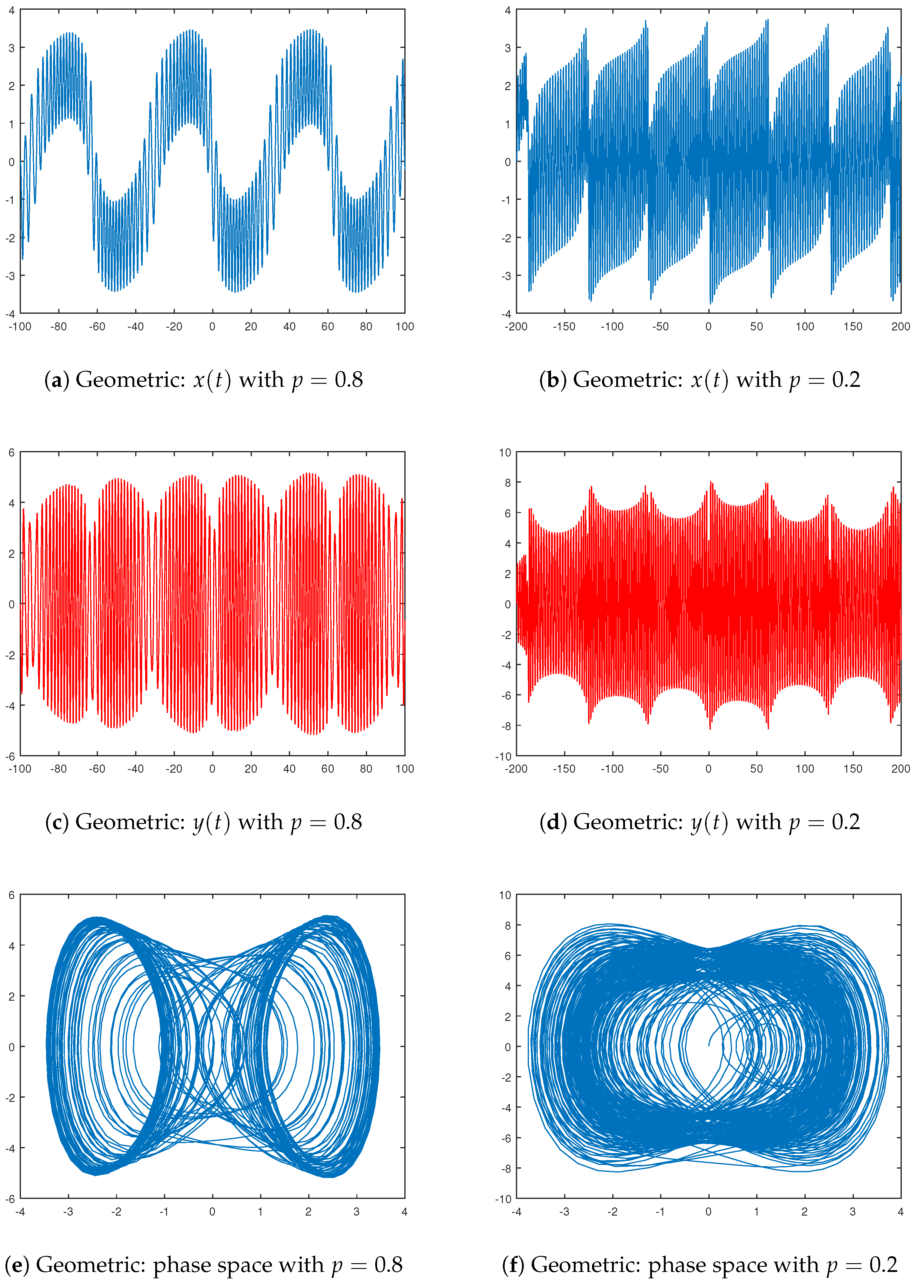
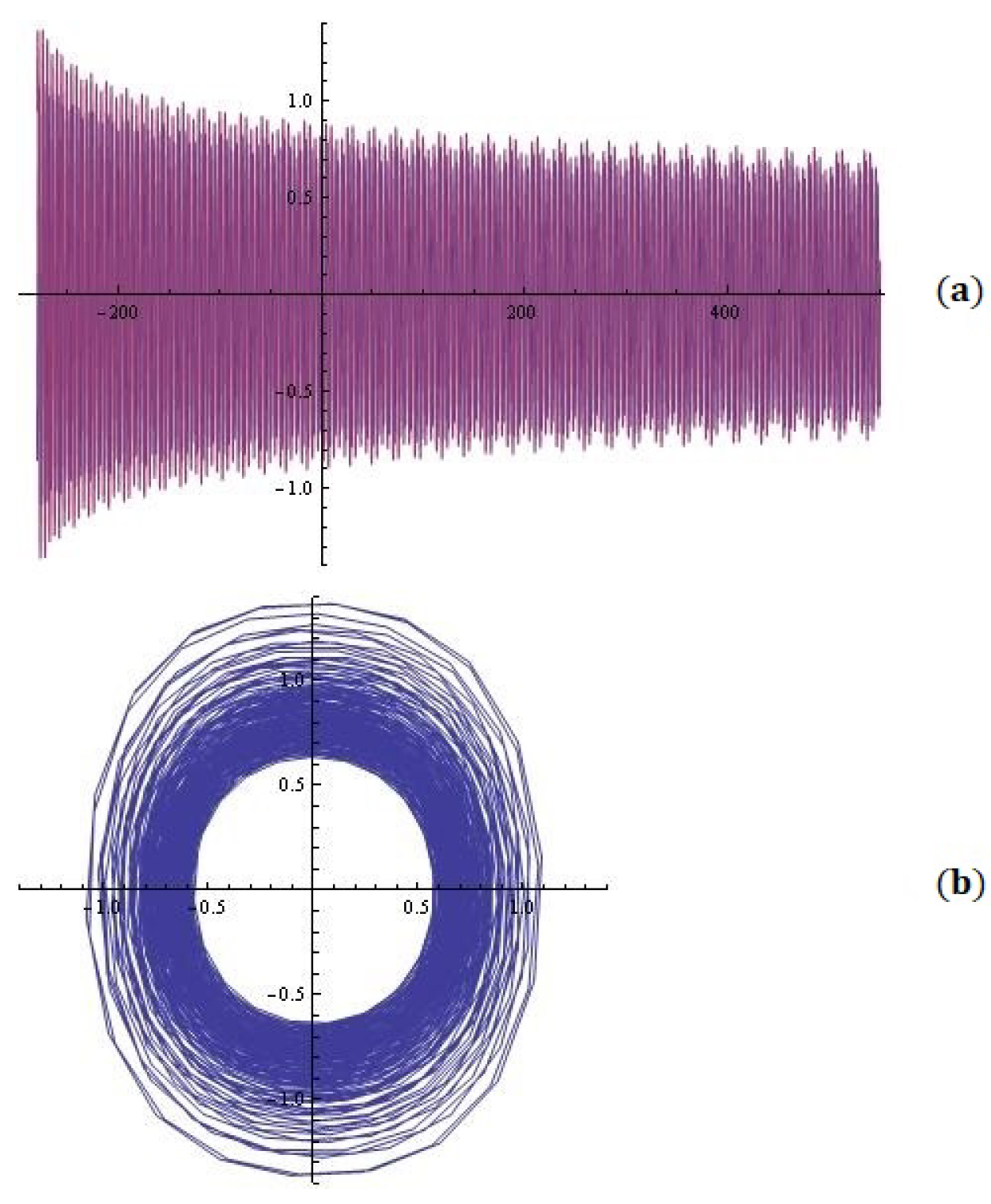
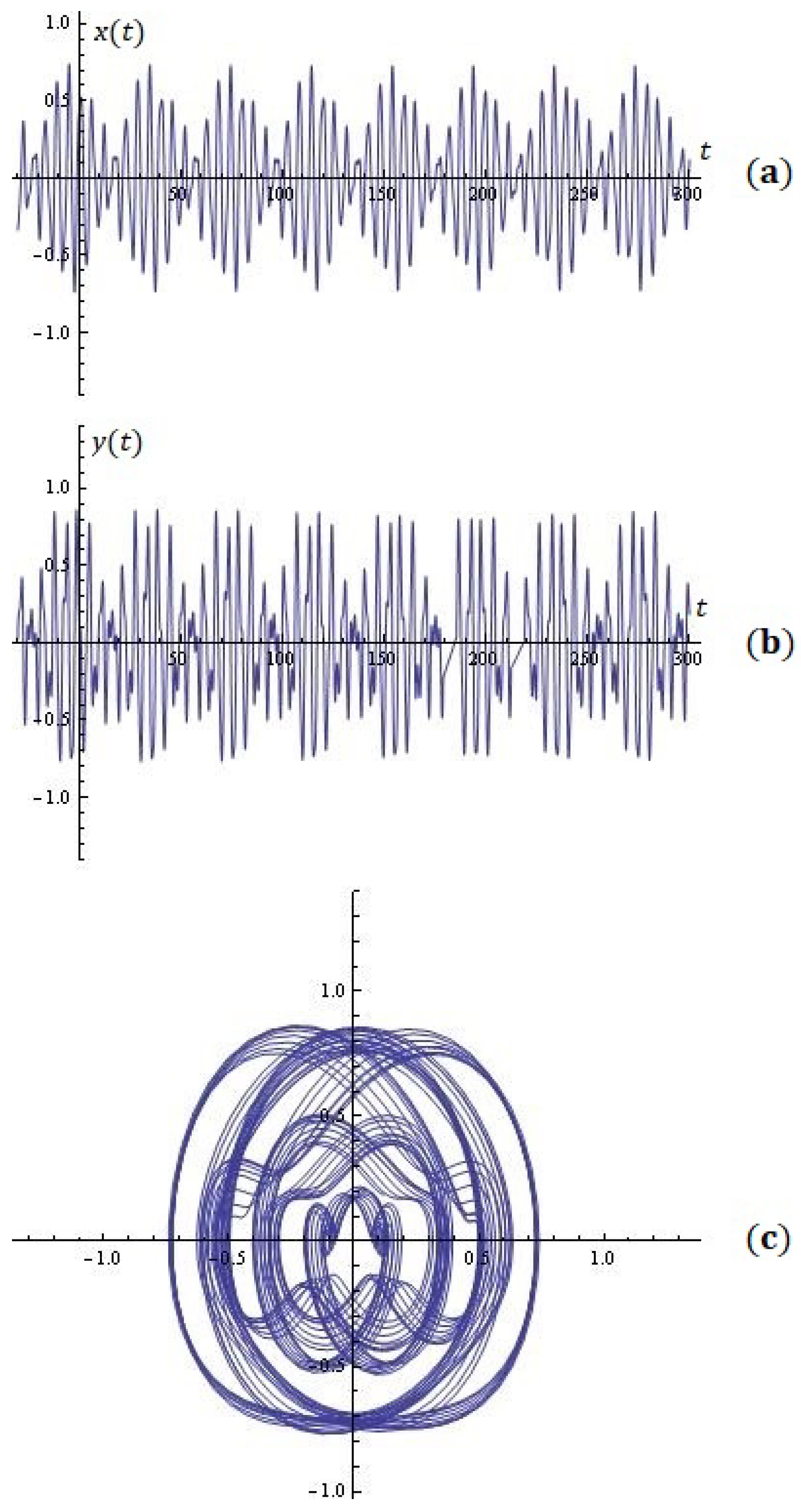
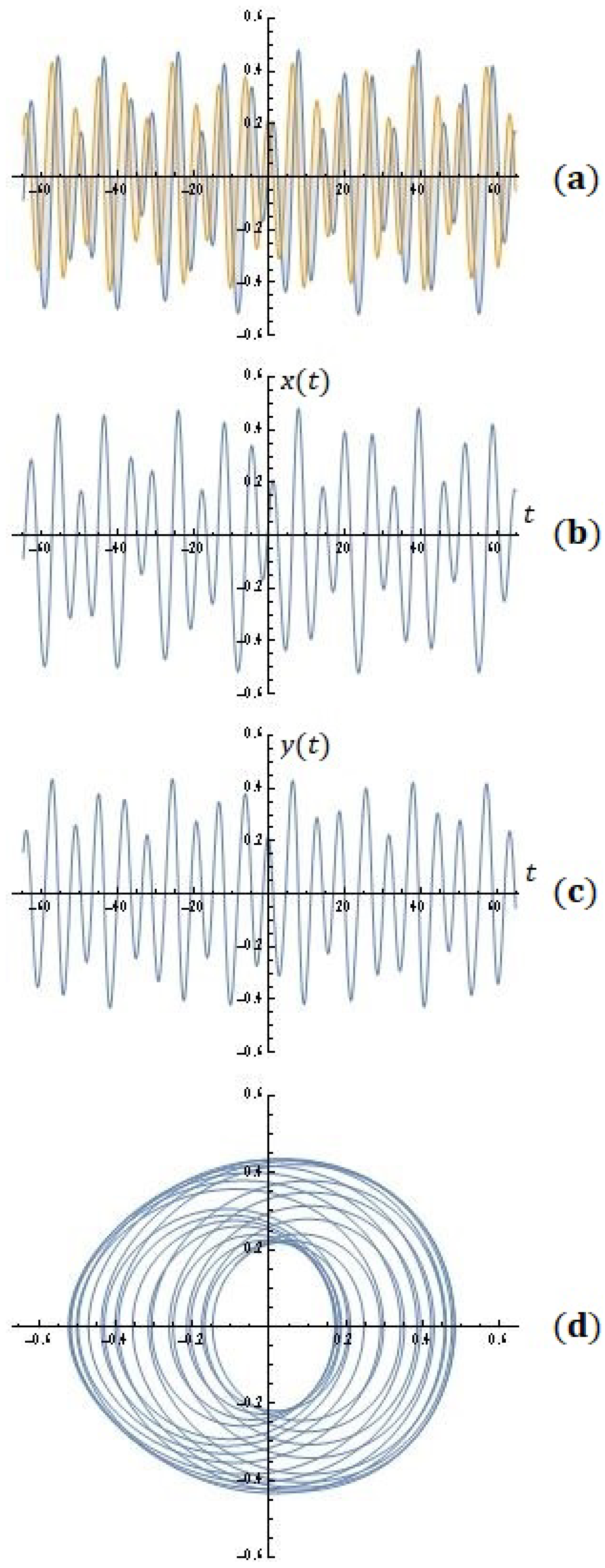
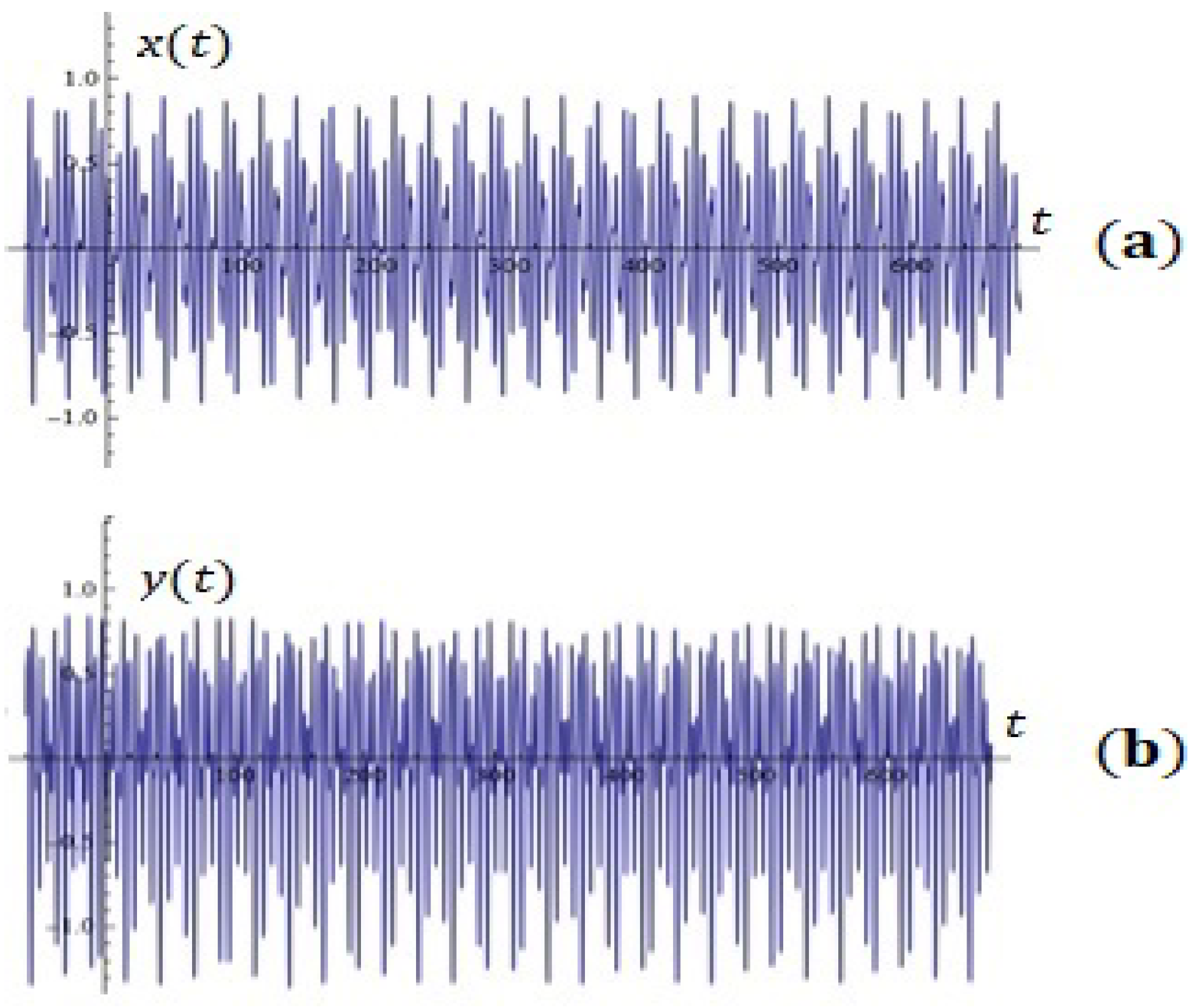
4. Some Simulations

For training purposes, we will look at some interesting simulations on models (10) and (11).

Example 1.

For given $p=6$, $N=1$, $A=0.5,ϵ=0.0085,\omega =0.9,$ and $g_1=3.7$, the simulations on system (10) for $x_0=0.7$ and $y_0=0.3$ are illustrated in Figure 12.

Example 2.

For given $p=10$, $N=3$, $A=0.05,ϵ=0.005,\omega =0.95,g_1=-15.5,g_2=-43.4,$ and $g_3=-73.5$, the simulations on system (10) for $x_0=0.4$ and $y_0=0.2$ are illustrated in Figure 13.

Example 3.

For given $p=4$, $N=1$, $A=0.052,ϵ=0.0085,\omega =0.6,$ and $g_1=12.7$, the simulations on system (11) for $x_0=0.1$ and $y_0=0.2$ are illustrated in Figure 14.

5. Recommended Training Tasks on the Topic of Chaos Generation

For training purposes, after Section 4, the following task can be set before trainees.

With an appropriate selection of the parameters of the considered differential model, perform the following:

(i)

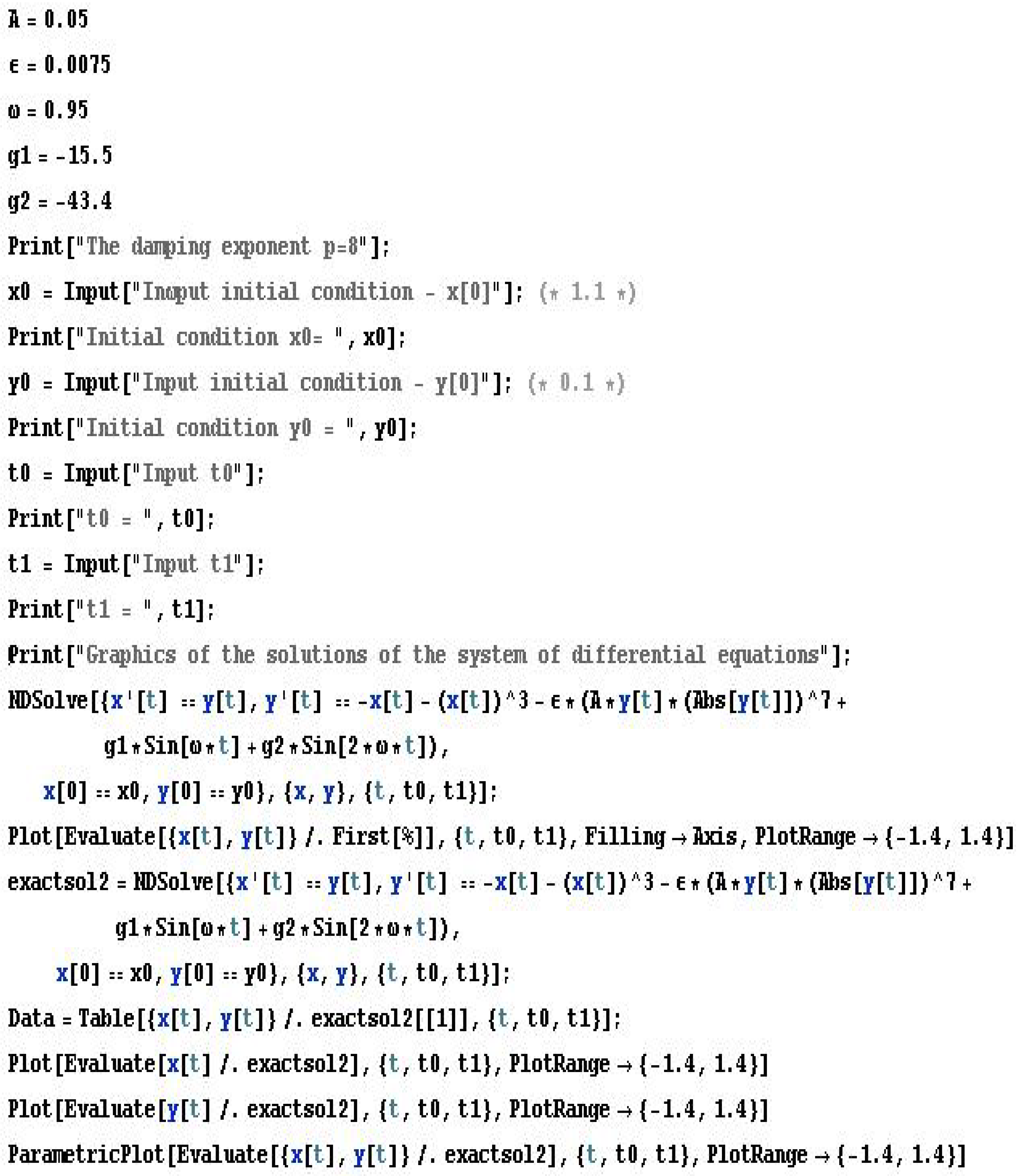
Generate chaos by using the learning module provided to you, implemented in Computer Algebraic System Mathematica for scientific computing (see Figure 15);

(ii)

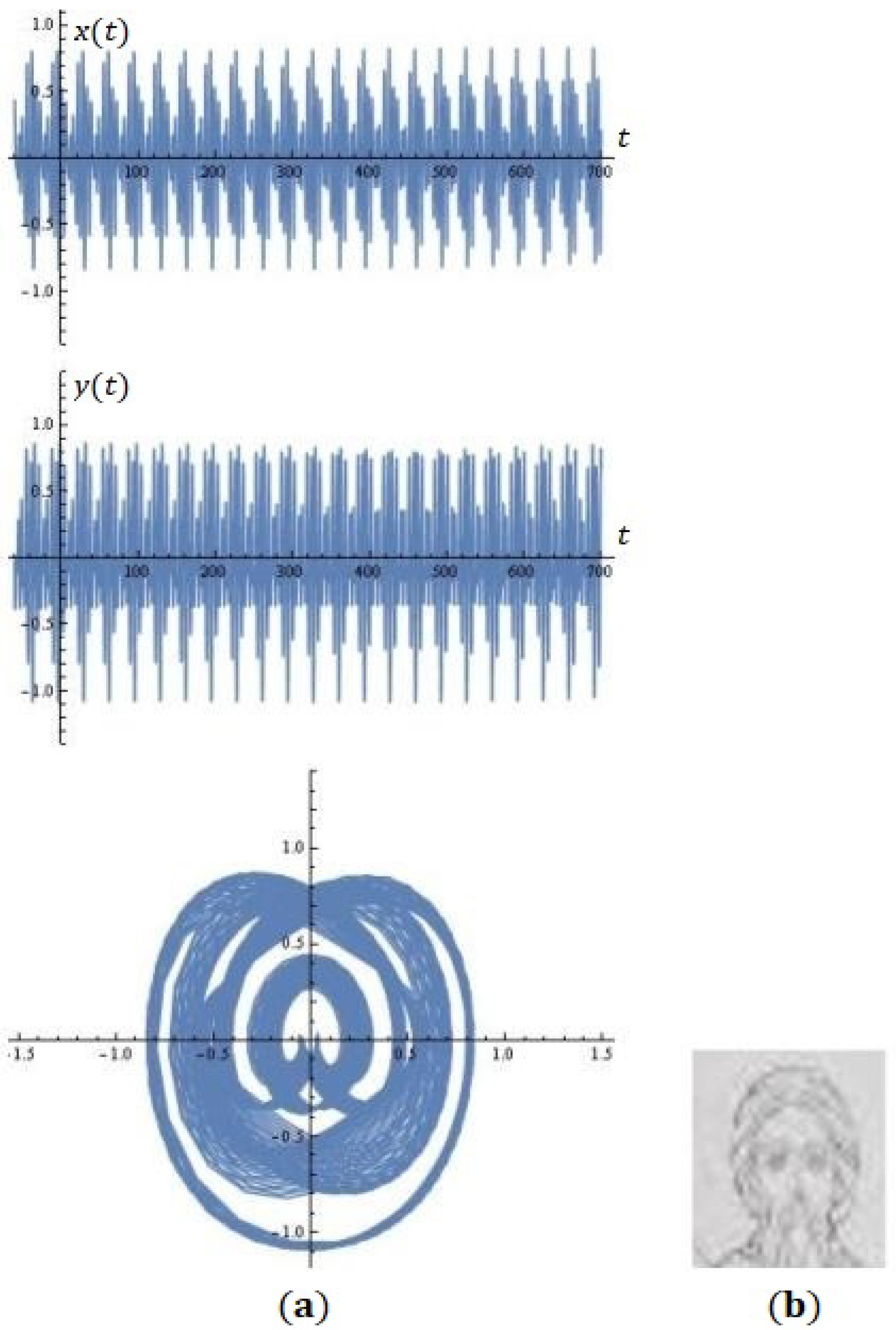
Indicate the values of the parameters at which the phase portrait approaches the illustration in Figure 16b (portrait of a Bulgarian saint);

(iii)

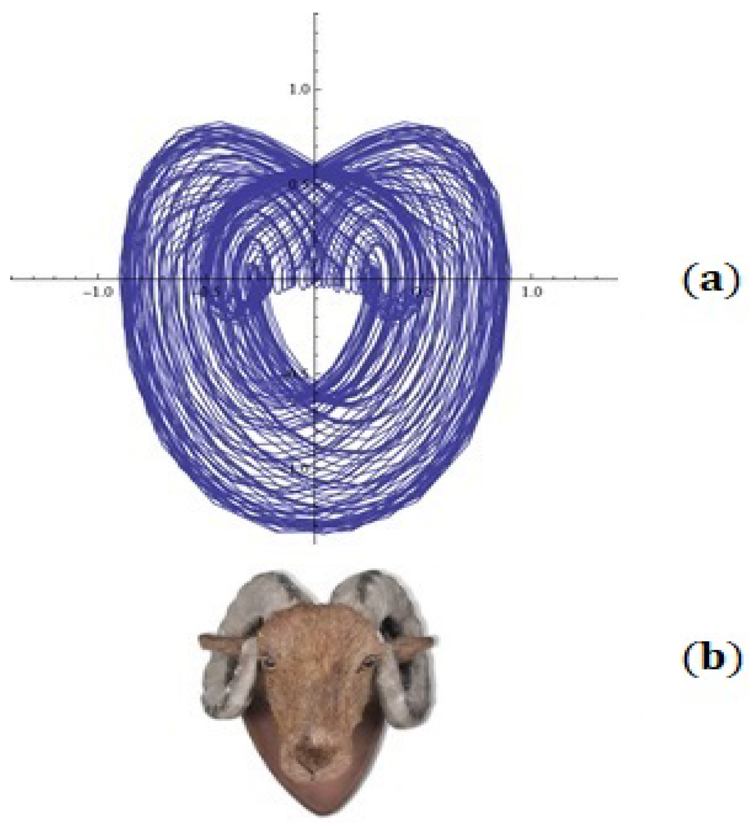
Indicate the values of the parameters at which the phase portrait approaches the illustration in Figure 17b (sheep’s head illustration);

(iv)

Draw appropriate conclusions.

• Guidance. (ii) A possible solution, for parameter values $p=8$, $N=2$, $A=0.05,$ $ϵ=0.0075,$ $\omega =0.95,g_1=-15.5,g_2=-43.4,x_0=0.5,$ and $y_0=0.2$ is visualized in Figure 16a. (iii) A possible solution, for parameter values $p=8$, $N=3$, $A=0.05,ϵ=0.0075,\omega =0.95,g_1=-25.5,$ $g_2=-50.4,g_3=50.9,x_0=0.4,$ and $y_0=0.15$ is visualized in Figure 18.

6. Conclusions

In this article, we give a new class of generalized differential models. We propose specific tools for researching the behavior of these systems. This will be a software module which will be a component of web-based tools through cloud computations. Our idea in this direction is to realize the goal of effective training with a specific focus on applications in entertainment, which motivates and stimulates learners towards the triad of enigmatics–creativity–acmeology. The above task is very instructive in several ways. First of all, learners should upgrade their proposed learning module in CAS Mathematica and make sure that a minimal change in the values of the many free parameters appearing in the explored model leads to interesting simulations. And the most important thing is that with the interesting teaching methodology proposed in this way, the students of master’s and doctoral programs will more easily touch upon the eternally relevant topic—generating chaos in modified classical and new differential models appearing in the literature. The study of models in terms of bifurcations, attractors, Lyapunov exponents, attractor merging, and amplitude control of hyperchaos [28,29] will be the subject of our future explorations.

Last but not least, we suggest that the coefficients that drive the perturbation be given by the probabilities of some discrete distribution after scaling. This way, we may introduce different weights having in mind the structural properties of the used distribution. Thus, we may impose a larger or smaller impact on the different parts of the oscillator dynamics. Also, we can use symmetric, asymmetric in both directions, highly asymmetric, or relatively uniform positions via the underlying distribution. Generally said, the variety of possible choices leads to a large flexibility of the proposed models.

We mentioned above some challenges for students and the opportunities we provide them with to explore the behavior of arbitrary models—generalizations of old and recent ones. However, teachers also face with serious challenges when they have to prepare topics for coursework of students from master’s and PhD programs on the subject—the subject of this article (albeit in a summarized form). The discussion of the achieved results of the methodological presentation of the subject matter offered in this article on the topic can be carried out only after the evaluation of the coursework of the students. In particular, it is about making modern GPT technologies, which are massively used by students for the realization of their coursework, as difficult as possible. And in order not to be surprised later by the finding of “plagiarism” (at this stage, the still proposed GPT implementations are a pale shadow of the real solutions, for example, those visualized in Figure 16 and Figure 17), we educators are obliged to set such tasks, which motivate and stimulate students towards the triad of enigmatics–creativity–acmeology.

We will be glad if this article provokes an interesting discussion in the pages of the authoritative journal Symmetry about the teaching methodology in this field of scientific knowledge.

References

- Georgieva, M.; Grozdev, S. Morphodynamics for the Development of Noospheric Intelligence; East-West Publishing House: Sofia, Bulgaria, 2016. (In Bulgarian) [Google Scholar]
- Guckenheimer, J.; Holmes, P. Nonlinear Oscillations, Dynamical Systems, and Bifurcations of Vector Fields; Springer: New York, NY, USA, 1983. [Google Scholar]
- Perko, L. Differential Equations and Dynamical Systems; Springer: New York, NY, USA, 1991. [Google Scholar]
- Blows, T.; Perko, L. Bifurcation of limit cycles from centers and separatix cycles of planar analytic systems. Siam Rev. 1994, 36, 341–371. [Google Scholar] [CrossRef]
- Byrd, P.; Friedman, M. Handbook of Elliptic Integrals for Scientist and Engineers; Springer: New York, NY, USA, 1971. [Google Scholar]
- Kyurkchiev, N.; Zaevski, T.; Iliev, A.; Kyurkchiev, V.; Rahnev, A. Modeling of Some Classes of Extended Oscillators: Simulations, Algorithms, Generating Chaos, and Open Problems. Algorithms 2024, 17, 121. [Google Scholar] [CrossRef]
- Sanjuan, M. The effect of nonlinear damping on the universal oscillator. Int. J. Bifurc. Chaos 1999, 9, 735–744. [Google Scholar] [CrossRef]
- Soliman, M.S.; Thompson, J.M.T. The effect of nonlinear damping on the steady state and basin bifurcation patterns of a nonlinear mechanical oscillator. Int. J. Bifurc. Chaos 1992, 2, 81–91. [Google Scholar] [CrossRef]
- Fangnon, R.; Ainamon, C.; Monwanou, A.V.; Mowadinou, C.H.; Orpu, J.B. Nonlinear dynamics of the quadratic damping Helmholtz oscillator. Complexity 2020, 2020, 8822534. [Google Scholar] [CrossRef]
- Bikdash, M.; Balachandran, B.; Nayfeh, A. Melnikov analysis for a ship with a general roll-damping model. Nonl. Dyn. 1994, 6, 101–124. [Google Scholar] [CrossRef]
- Ravindra, B.; Mallik, A.K. Stability analysis of a non–linearly clamped Duffing oscillator. J. Spund Vib. 1999, 171, 708–716. [Google Scholar] [CrossRef]
- Ravindra, B.; Mallik, A.K. Role of nonlinear dissipation in soft Duffing oscillators. Phys. Rev. E 1984, 49, 4950–4954. [Google Scholar] [CrossRef]
- Sanjuan, M. Monoclinic bifurcation sets of driven nonlinear oscillators. Int. J. Theroetical Phys. 1996, 35, 1745–1752. [Google Scholar] [CrossRef]
- Holmes, P.; Marsden, J. Horseshoes in perturbation of Hamiltonian systems with two degrees of freedom. Comm. Math. Phys. 1982, 82, 523–544. [Google Scholar] [CrossRef]
- Holmes, P.; Marsden, J. A partial differential equation with infinitely many periodic orbits: Chaotic oscillations. Arch. Ration. Mech. Anal. 1981, 76, 135–165. [Google Scholar] [CrossRef]
- Francescatto, A.; Contento, G. Bifurcations in ship rolling: Experimental results and parameter identification technique. Ocean Eng. 1999, 26, 1095–1123. [Google Scholar] [CrossRef]
- Tang, K.; Man, K.; Zhong, G.; Chen, G. Generating chaos via x|x|. IEEE Trans. Circuit Syst. I Fundam. Theory Appl. 2001, 48, 636–640. [Google Scholar] [CrossRef]
- Levi, M.; Hoppensteadt, F.; Miranker, W. Dynamics of the Josephson junction. Quart. Appl. Math. 1978, 35, 167–198. [Google Scholar] [CrossRef]
- Siewe, M.; Kakmeni, F.; Tchawoua, C. Resonant oscillation and homoclinic bifurcation in ϕ6—Van der Pol oscillator. Chaos Solut. Fractals 2004, 21, 841–853. [Google Scholar] [CrossRef]
- Yu, J.; Li, J. Investigation on dynamics of the extended Duffing-Van der Pol system. Zetschrift Naturforschung 2009, 64, 341–346. [Google Scholar] [CrossRef]
- Siewe, M.; Tchawoua, C.; Rajasekar, S. Homoclinic bifurcation and chaos in ϕ6 Rayleigh oscillator with three wells driven by an amplitude modulated force. Int. J. Bifurc. Chaos 2011, 21, 1583–1593. [Google Scholar] [CrossRef]
- Lenci, S.; Rega, G. Controlling nonlinear dynamics in a two-well impact system. I. Attractors and bifurcation scenario under symmetric excitations. Int. J. Bifur. Chaos 1998, 8, 2387–2407. [Google Scholar] [CrossRef]
- Lenci, S.; Rega, G. Controlling nonlinear dynamics in a two-well impact system. II. Attractors and bifurcation scenario under unsymmetric optimal excitation. Int. J. Bifur. Chaos 1998, 8, 2409–2424. [Google Scholar] [CrossRef]
- Soto-Trevino, C.; Kaper, T.J. Higher-order Melnikov theory for adiabatic systems. J. Math. Phys. 1996, 37, 6220–6249. [Google Scholar] [CrossRef]
- Yagasaki, K. Melnikov’s method and codimension–two bifurcation in forced oscillations. J. Differ. Equ. 2002, 185, 1–24. [Google Scholar] [CrossRef]
- Yagasaki, K. Melnikov theory for subharmonics and their bifurcations in forced oscillations. SIAM J. Appl. Math. 1996, 56, 1720–1765. [Google Scholar] [CrossRef]
- Gavrilov, L.; Iliev, I. The limit cycles in a generalized Rayleigh-Lienard oscillator. Discret. Contin. Dyn. Syst. 2023, 43, 2381–2400. [Google Scholar] [CrossRef]
- Li, Y.; Li, C.; Zhong, Q.; Tengfei, L.; Sicong, L. Attractor Merging and Amplitude Control of Hyperchaos in a Self-Reproducing Memristive Map. Int. J. Bifurc. Chaos 2024, 34, 2450050. [Google Scholar] [CrossRef]
- Li, Y.; Li, C.; Zhong, Q.; Sicong, L.; Tengfei, L. A memristive chaotic map with only one bifurcation parameter. Nonlinear Dyn. 2024, 112, 3869–3886. [Google Scholar] [CrossRef]
Disclaimer/Publisher’s Note: The statements, opinions and data contained in all publications are solely those of the individual author(s) and contributor(s) and not of MDPI and/or the editor(s). MDPI and/or the editor(s) disclaim responsibility for any injury to people or property resulting from any ideas, methods, instructions or products referred to in the content. |
© 2024 by the authors. Licensee MDPI, Basel, Switzerland. This article is an open access article distributed under the terms and conditions of the Creative Commons Attribution (CC BY) license (https://creativecommons.org/licenses/by/4.0/).
Share and Cite
Kyurkchiev, N.; Zaevski, T.; Iliev, A.; Kyurkchiev, V.; Rahnev, A. Generating Chaos in Dynamical Systems: Applications, Symmetry Results, and Stimulating Examples. Symmetry 2024, 16, 938. https://doi.org/10.3390/sym16080938
Kyurkchiev N, Zaevski T, Iliev A, Kyurkchiev V, Rahnev A. Generating Chaos in Dynamical Systems: Applications, Symmetry Results, and Stimulating Examples. Symmetry. 2024; 16(8):938. https://doi.org/10.3390/sym16080938
Chicago/Turabian StyleKyurkchiev, Nikolay, Tsvetelin Zaevski, Anton Iliev, Vesselin Kyurkchiev, and Asen Rahnev. 2024. "Generating Chaos in Dynamical Systems: Applications, Symmetry Results, and Stimulating Examples" Symmetry 16, no. 8: 938. https://doi.org/10.3390/sym16080938