Dual-Loop μ-Synthesis Direct Thrust Control for Turbofan Engines

Abstract

As the power unit of an aircraft, the engine’s primary task is to provide the demanded thrust, making research on direct thrust control crucial. However, being a complicated multivariable system, effective multivariable direct thrust control methods are currently lacking. The main content of this paper is threefold. First, it presents a dual-loop multivariable μ-synthesis direct thrust control scheme for mixed-exhaust low-bypass turbofan engines, which is a typical rotationally symmetric machine. The scheme adjusts fuel flow for thrust control and nozzle area to control the turbine pressure ratio, ensuring thrust tracking while maintaining the engine’s key parameters within safe limits. Second, a fast, accurate thrust estimation algorithm based on aerodynamic thermodynamics and component characteristics is introduced. At last, considering the model uncertainties between off-design and design points, a weight function frequency shaping μ-synthesis control design method is proposed to address internal loop coupling and external disturbance suppression. Nonlinear simulations within the flight envelope show that μ-synthesis direct thrust control achieves robust servo tracking and disturbance rejection, with a maximum steady-state thrust error of no more than 0.1%, and the key parameters are not over their safety boundaries.

1. Introduction

With the advancement of aero-engine control technology, direct thrust control has become a hot and challenging topic [1,2,3]. Previously, indirect thrust control schemes based on rotor speed were used due to the inability to measure thrust [4]. Thrust should correspond linearly with the power lever angle, but the nonlinear relationship between rotor speed and thrust only allows for an approximate linear relationship, increasing the pilot’s workload [5]. Moreover, as engine performance degrades over its service life, these nonlinear characteristics become even more pronounced [6].

Scholars worldwide have extensively researched direct thrust control for engines. Litt et al. proposed a Kalman filter thrust estimator [7]. They used an indirect thrust control method, correcting fan speed commands based on the deviation between the desired thrust and the Kalman filter estimate [8]. However, this approach cannot ensure a linear relationship between thrust and the power lever. Lu et al. studied methods for estimating engine health parameters under sensor uncertainty [9,10]. Francisco et al. proposed a direct thrust control scheme for turbojet engines using an optimal linear quadratic (LQ) fuel consumption index and an optimal thrust estimator [11]. With the development of artificial intelligence (AI) technology, data-driven thrust estimation methods have emerged. Algorithms such as support vector machines [12,13], multilayer feedforward neural networks [14], extreme learning machines [15,16], radial basis function neural networks [17,18], deep convolutional neural networks [19], and long short-term memory neural networks [20] have been applied to engine thrust estimation. However, these methods require extensive thrust data covering the entire flight envelope and various environmental conditions, which are nearly impossible to obtain, making practical application challenging.

Wang developed a turbofan engine thrust estimator using the optimal unknown input observer (UIO) method and proposed a model-based dual-loop thrust control structure with closed-loop feedback [21]. The inner loop employs H-infinity loop-shaping rotor speed control, while the outer loop uses anti-windup proportional–integral (PI) thrust control. Zheng et al. proposed a real-time optimization control method to enhance engine thrust response during emergency flights [22]. They later introduced a nonlinear model predictive control method for direct thrust, improving thrust response speed by 50% [23]. Additionally, they developed an inverse mapping model for direct thrust control [24], which ensures desired thrust and rapid response even with engine degradation. Jin et al. proposed an aircraft engine direct thrust prediction control method based on a composite propulsion system dynamic model–state variable model [25]. This approach allows for simultaneous estimation of unmeasured parameters and model predictive control, improving steady-state control accuracy and effectiveness. Zhu et al. [26] proposed a direct thrust control structure based on linear parameter varying (LPV) for turbofan engines. Their robust filtering estimator effectively suppresses sensor noise, and the designed optimal controller shows ideal performance above idle. However, these methods may not perform as expected in the face of uncertainties and external disturbances.

There are many ways to cope with uncertainties and external disturbances, such as robust control, adaptive control, etc. [27,28]. Liu et al. [29] proposed a multi-variable adaptive control method for turbofan engines to deal with the dynamic and input uncertainties. Shi et al. [30] studied supervisory control of multiple switching laws with performance guidance for aero-engines. Xiao [31] proposed a novel nonlinear tracking control for aero-engines to suppress the effects of uncertainties and disturbances. In addition, the H∞ and μ-synthesis techniques show strong robustness and ability to suppress external disturbances [32,33]. Wang et al. designed a two-degrees-of-freedom H∞ controller for aero-engines to improve the tracking performance while maintaining stability and robustness [34]. Compared to H∞ control, the µ-synthesis control is able to deal with uncertainties directly. However, µ-synthesis has been less studied in direct thrust control of aero-engines.

In order to solve these issues mentioned above, the research presented in this paper provides the following main contributions:

• To address the issue of poor linearity between power lever angle and thrust in indirect thrust control schemes, this paper proposes a multivariable direct thrust control structure that ensures thrust tracking while using nozzle adjustments to regulate the pressure ratio, preventing key performance parameters from exceeding their limits.
• To solve the problem of unmeasurable thrust and to avoid the difficulty in obtaining thrust data for data-driven algorithms, a fast thrust estimation algorithm based on measurable parameters and engine thermodynamic characteristics is introduced to act as a virtual thrust sensor.
• To tackle external disturbances and uncertainties in direct thrust control, a dual-loop μ-synthesis multivariable direct thrust control method is designed.

This study explores direct thrust control in mixed-exhaust small bypass ratio turbofan engines. Firstly, it analyzes the impact of nozzle area changes on engine operation and proposes a dual-loop direct thrust control scheme. The nozzle control loop adjusts the nozzle area to maintain the turbine pressure ratio relative to changes in inlet total temperature, while the fuel control loop adjusts fuel flow to maintain thrust relative to inlet total temperature changes. Secondly, it introduces a rapid thrust estimation algorithm based on engine principles using aerodynamic thermodynamics and component characteristics. Thirdly, a weighted function frequency domain shaping μ-synthesis control method is proposed to address uncertainty between non-design and design operating points in the engine’s full envelope. This method ensures robustness for controllers designed at design points within the uncertainty range, providing robust and anti-disturbance performance for direct thrust control across flight envelopes. Finally, simulation verification on a nonlinear engine platform validates the servo and anti-disturbance performance.

2. Design Methods

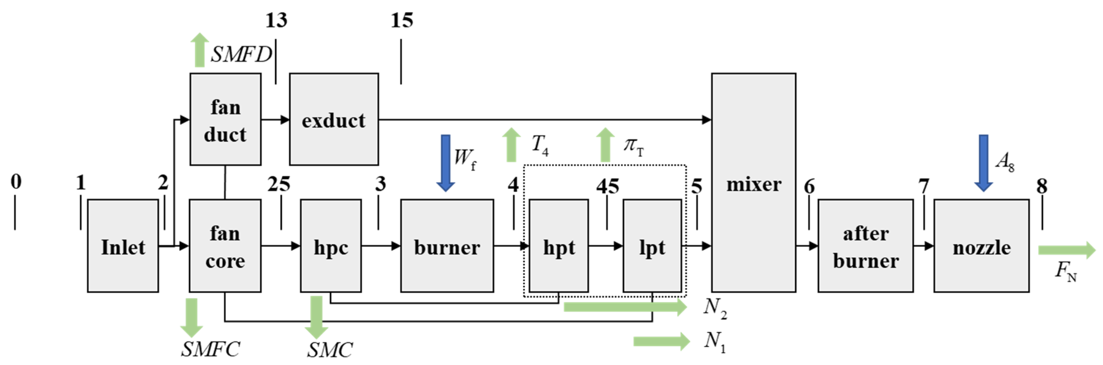
2.1. Augmented Engine Model

The state space nonlinear model of a small bypass ratio dual-axis turbofan engine (the schematic diagram is shown in Figure 1) is described [3,4] as

$$\{\begin{array}{c}\dot{x}(t)=f\left(x(t),u(t)\right)\\ y(t)=g\left(x(t),u(t)\right)\end{array}$$

(1)

where state variable $x={\left[\begin{array}{cc}{x}_1& x_2\end{array}\right]}^{\mathrm{T}}={\left[\begin{array}{cc}{N}_1& N_2\end{array}\right]}^{\mathrm{T}}$; $N_1$ (unit: rpm) and $N_2$ (unit: rpm) are the low-pressure and high-pressure rotor speeds of the engine, respectively; input variable $u={\left[\begin{array}{cc}{u}_1& u_2\end{array}\right]}^{\mathrm{T}}={\left[\begin{array}{cc}{W}_{\mathrm{f}}& A_8\end{array}\right]}^{\mathrm{T}}$ (units: kg/s and m²), $W_{\mathrm{f}}$ means the fuel flow rate and $A_8$ means the nozzle throat area; the output variable $y={\left[\begin{array}{ccc}{F}_{\mathrm{N}}& {\pi }_{\mathrm{T}}& y_{\mathrm{ex}}\end{array}\right]}^{\mathrm{T}}$, where $F_{\mathrm{N}}$ (unit: N) is engine net thrust, ${\pi }_{\mathrm{T}}$ is turbine pressure ratio, and $y_{\mathrm{ex}}$ represents other monitoring outputs, including some engine aerodynamic and thermal parameters; f represents nonlinear mappings from x, u to $\dot{x}$; and g represents nonlinear mappings from x, u to y.

The transformation matrix of state, input, and output is defined as

$$T{M}_x=\mathrm{diag}(x_{\mathrm{design}}^{-1}), T{M}_u=\mathrm{diag}(u_{\mathrm{design}}^{-1}), T{M}_y=\mathrm{diag}(y_{\mathrm{design}}^{-1})$$

(2)

where the subscript “design” represents the design point of the engine.

We can transform the state vector, input vector, and output vector as follows:

$$\dot{\overline{x}}(t)=T{M}_x\dot{x}(t),\overline{x}(t)=T{M}_{x}x\left(t\right),\overline{u}(t)=T{M}_{u}u(t),\overline{y}(t)=T{M}_{y}y(t)$$

(3)

Equation (1) can be transformed into the following normalized state space nonlinear model:

$$\{\begin{array}{c}\dot{\overline{x}}(t)=\overline{f}\left(\overline{x}(t),\overline{u}(t)\right)\\ \overline{y}(t)=\overline{g}\left(\overline{x}(t),\overline{u}(t)\right)\end{array}$$

(4)

where $\overline{f}$ is a nonlinear mapping function from $\overline{x},\overline{u}$ to $\dot{\overline{x}}$, and $\overline{g}$ is a nonlinear mapping function from $\overline{x},\overline{u}$ to $\overline{y}$.

Linearizing the nonlinear model at a steady-state point and expanding Equation (4) in terms of the Taylor series of multivariate functions yields the linear model.

$$G_{\mathrm{engine}}:\{\begin{array}{c}\Delta \dot{\overline{x}}(t)=A\Delta \overline{x}(t)+B\Delta \overline{u}(t)\\ \Delta \overline{y}(t)=C\Delta \overline{x}(t)+D\Delta \overline{u}(t)\end{array}$$

(5)

where

$$\begin{array}{c}A={\left[\begin{array}{cc}{\displaystyle \frac{\partial {\overline{f}}_1}{\partial {\overline{x}}_1}}& {\displaystyle \frac{\partial {\overline{f}}_1}{\partial {\overline{x}}_2}}\\ {\displaystyle \frac{\partial {\overline{f}}_2}{\partial {\overline{x}}_1}}& {\displaystyle \frac{\partial {\overline{f}}_2}{\partial {\overline{x}}_2}}\end{array}\right]}_{|x_0,u_0},B={\left[\begin{array}{cc}{\displaystyle \frac{\partial {\overline{f}}_1}{\partial {\overline{u}}_1}}& {\displaystyle \frac{\partial {\overline{f}}_1}{\partial {\overline{u}}_2}}\\ {\displaystyle \frac{\partial {\overline{f}}_2}{\partial {\overline{u}}_1}}& {\displaystyle \frac{\partial {\overline{f}}_2}{\partial {\overline{u}}_2}}\end{array}\right]}_{|x_0,u_0}\\ C={\left[\begin{array}{cc}{\displaystyle \frac{\partial {\overline{g}}_1}{\partial {\overline{x}}_1}}& {\displaystyle \frac{\partial {\overline{g}}_1}{\partial {\overline{x}}_2}}\\ {\displaystyle \frac{\partial {\overline{g}}_2}{\partial {\overline{x}}_1}}& {\displaystyle \frac{\partial {\overline{g}}_2}{\partial {\overline{x}}_2}}\end{array}\right]}_{|x_0,u_0},D={\left[\begin{array}{cc}{\displaystyle \frac{\partial {\overline{g}}_1}{\partial {\overline{u}}_1}}& {\displaystyle \frac{\partial {\overline{g}}_1}{\partial {\overline{u}}_2}}\\ {\displaystyle \frac{\partial {\overline{g}}_2}{\partial {\overline{u}}_1}}& {\displaystyle \frac{\partial {\overline{g}}_2}{\partial {\overline{u}}_2}}\end{array}\right]}_{|x_0,u_0}\end{array}$$

Considering that both dual-loop actuators engage a small closed-loop control mode, their equivalent first-order inertial modules are

$$G_{W_{\mathrm{f}}}\left(s\right)={\displaystyle \frac{1}{{\tau }_{W_{\mathrm{f}}}s+1}},G_{A_8}(s)={\displaystyle \frac{1}{{\tau }_{A_8}s+1}}$$

(6)

${\tau }_{W_{\mathrm{f}}}$ is the equivalent inertia time constant of the fuel actuator and ${\tau }_{A_8}$ is the equivalent inertia time constant of the nozzle actuator.

Direct engine thrust control has servo performance requirements. According to the automatic control principle, it is necessary to contain an integrator in the forward channel of the control loop; therefore, the following integrator is embedded:

$$G_{W_{\mathrm{f}},\mathrm{inte}}(s)={\displaystyle \frac{1}{s}},G_{A_8,\mathrm{inte}}(s)={\displaystyle \frac{1}{s}}$$

(7)

So far, the augmented controlled object model is constructed as follows:

$$G_{\mathrm{Aug}}=G_{\mathrm{engine}}\cdot \left[\begin{array}{cc}{G}_{W_{\mathrm{f}}}& 0\\ 0& G_{A_8}\end{array}\right]\cdot \left[\begin{array}{cc}{G}_{W_{\mathrm{f}},\mathrm{inte}}& 0\\ 0& G_{A_8,\mathrm{inte}}\end{array}\right]$$

(8)

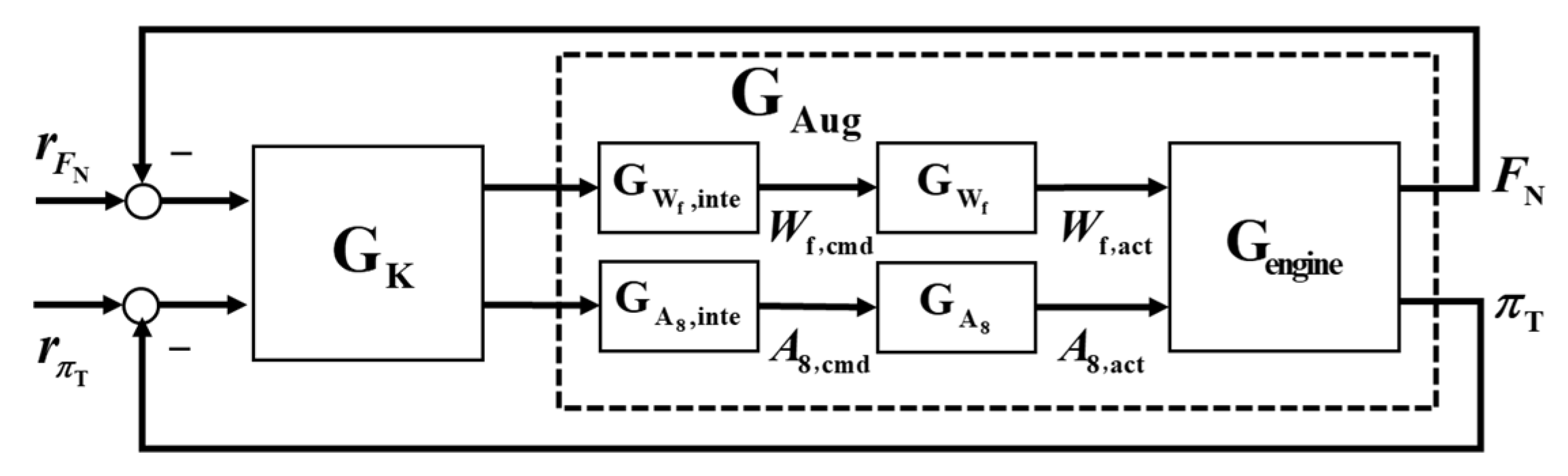
2.2. Direct Thrust Dual-Loop Control Scheme

At present, the thrust control of an aircraft engine is completed by an indirect thrust control mode, which utilizes the rotor speed closed-loop. With this traditional control scheme, it is difficult to ensure that the thrust linearly corresponds to the power lever angle. With the growing engine operating cycles, the nonlinearity between the thrust and the power lever angle becomes more obvious, aggravating the pilot’s maneuvering load.

In the process of engine transition state and steady-state operation, the change in the nozzle throat area directly affects the position of the common operating point. In order to ensure the safe operation of the engine, the operating point should maintain a certain safety margin with the safety boundaries, such as the fan, compressor unstable boundaries, the high-pressure turbine inlet temperature limitation boundaries, and the combustor lean blowout boundaries. Considering this characteristic, a direct thrust dual-loop control scheme is proposed, as shown in Figure 2.

In Figure 2, the upper loop receives the thrust command corresponding to the angle of the power lever and adopts the closed-loop structure of adjusting the fuel flow to control the thrust; the lower one receives the turbine pressure ratio command corresponding to the angle of the power lever and adopts the closed-loop structure of adjusting the nozzle throat area to control the turbine pressure ratio, and the internal coupling of loops 1 and 2 is solved by the multivariable controller to realize dynamic decoupling.

2.3. Thrust Estimation Algorithm

In Figure 2, the direct thrust dual-loop closed-loop control system scheme requires a thrust sensor; however, considering that the actual thrust is not measurable, the following thrust estimation algorithm based on measurable parameters and engine thermodynamic characteristics is proposed here.

We use the low-pressure rotor speed $N_1$ and fan inlet total temperature $T_2$ (unit: K) to calculate the low-pressure rotor corrected speed:

$$N_{1,\mathrm{cor}}=N_1/\sqrt{T_2/288.15}$$

(9)

Knowing the fan inlet total pressure $P_2$ (unit: kPa) and the fan bypass outlet total pressure $P_{13}$ (unit: kPa), the fan bypass pressure ratio can be obtained:

$${\pi }_{\mathrm{fanduct}}=P_{13}/P_2$$

(10)

Based on the fan bypass component characteristics,

$$\left[W_{\mathrm{fanduct},\mathrm{cor}},{\eta }_{\mathrm{fanduct}}\right]=f_{\mathrm{fanduct}}(N_{1,\mathrm{cor}},{\pi }_{\mathrm{fanduct}})$$

(11)

$W_{\mathrm{fanduct},\mathrm{cor}}$ (unit: kg/s), ${\eta }_{\mathrm{fanduct}}$ can be calculated, and thus the fan bypass inlet air flow rate $W_{\mathrm{fanduct}}$(unit: kg/s) is

$$W_{\mathrm{fanduct}}=W_{\mathrm{fanduct},\mathrm{cor}}\cdot {\displaystyle \frac{\sqrt{288.15/T_2}}{101.325/P_2}}$$

(12)

The fan bypass outlet total temperature is

$$T_{13}=T_2(1+{\displaystyle \frac{{\pi }_{\mathrm{fanduct}}^{\frac{k-1}{k}}-1}{{\eta }_{\mathrm{fanduct}}}})$$

(13)

where k represents the air insulation index. Summarizing the above leads to a computational module for $W_{\mathrm{fanduct}},W_{13},T_{13}$ (units: kg/s, kg/s and K).

$$\left[W_{\mathrm{fanduct}},W_{13},T_{13}\right]={\mathrm{Fun}}_{\mathrm{fanduct}}(N_1,P_2,P_{13},T_2)$$

(14)

4.

The fan core thermal parameter calculation is similar to Step 1. From $N_1$, $P_2$, fan core outlet total pressure $P_{25}$ (unit: kPa), $T_2$, and fan core component characteristics, we can obtain the inlet flow rate $W_{\mathrm{fancore}}$ (unit: kg/s), outlet flow rate $W_{25}$ (unit: kg/s), and outlet total temperature $T_{25}$ (unit: K).

$$\left[W_{\mathrm{fancore}},W_{25},T_{25}\right]={\mathrm{Fun}}_{\mathrm{fanc}}(N_1,P_2,P_{25},T_2)$$

(15)

5.

The fan inlet air flow rate is obtained from Equations (14) and (15).

$$W_2=W_{\mathrm{fanduct}}+W_{\mathrm{fancore}}$$

(16)

6.

Considering the extracted air flow rate $W_{\mathrm{extr}}$ (unit: kg/s) from the compressor, then

$$W_3=W_{25}-W_{\mathrm{extr}}$$

(17)

The calculation of other thermal parameters is similar to Step 1. From the high-pressure rotor speed $N_2$, $P_{25}$, the total pressure at the outlet of the compressor $P_3$ (unit: kPa), $T_{25}$, and the characteristics of high-pressure compressor components, the inlet air flow rate of the compressor $W_{25}$, the outlet air flow rate of the compressor $W_3$ (unit: kg/s), and the total temperature at the outlet of the compressor $T_3$ (unit: K) can be obtained.

$$[W_{25},W_3,T_3]={\mathrm{Fun}}_{\mathrm{hpc}}(N_2,P_{25},P_3,T_{25},W_{\mathrm{extr}})$$

(18)

7.

From $W_3,P_3,T_3$, and the fuel flow rate $W_{\mathrm{f}}$, we obtain the fuel–air ratio and the gas flow rate at the outlet of the combustion chamber.

$$FA{R}_4=W_{\mathrm{f}}/W_3$$

(19)

$$W_4=W_3+W_{\mathrm{f}}$$

(20)

The combustion efficiency ${\eta }_B$ and the low-level calorific value $Hu$ (unit: J/kg) of the fuel are known, from which the total temperature at the outlet of the combustion chamber is calculated.

$$T_4={\displaystyle \frac{{\eta }_B\cdot FA{R}_4\cdot Hu+C{p}_3\cdot T_3}{(FA{R}_4+1)\cdot C{p}_4}}$$

(21)

where $C{p}_3$ (unit: J/K) is the constant-pressure specific heat capacity of air and $C{p}_4$ (unit: J/K) is the constant-pressure specific heat capacity of gas; then, the combustion chamber calculation module is

$$\left[W_4,T_4,FA{R}_4\right]={\mathrm{Fun}}_{\mathrm{burner}}(W_3,P_3,T_3,W_{\mathrm{f}})$$

(22)

8.

Considering the high-pressure turbine cooling air flow rate is $W_{\mathrm{hpt},\mathrm{cool}}$ (unit: kg/s), then the high-pressure turbine outlet gas flow rate is

$$W_{45}=W_4+W_{\mathrm{hpt},\mathrm{cool}}$$

(23)

The fuel–air ratio at the high-pressure turbine outlet is

$$FA{R}_{45}=W_{\mathrm{f}}/(W_{45}-W_{\mathrm{f}})$$

(24)

The corrected high-pressure turbine rotor speed is calculated from $N_2,T_4$ (units: K):

$$N_{2,\mathrm{cor},\mathrm{hpt}}=N_2/\sqrt{T_4/288.15}$$

(25)

From the high-pressure turbine inlet total pressure $P_4$ (unit: kPa) and outlet total pressure $P_{45}$ (unit: kPa), the high-pressure turbine pressure ratio is calculated:

$${\pi }_{\mathrm{hpt}}=P_4/P_{45}$$

(26)

Based on the characteristics of the high-pressure turbine components, $N_{2,\mathrm{cor},\mathrm{hpt}}$ (unit: rpm), and ${\pi }_{\mathrm{hpt}}$, parameters of the high-pressure turbine can be obtained:

$$\left[W_{\mathrm{hpt},\mathrm{cor}},{\eta }_{\mathrm{hpt}}\right]=f_{\mathrm{hpt}}(N_{2,\mathrm{cor},\mathrm{hpt}},{\pi }_{\mathrm{hpt}})$$

(27)

$$T_{45}=T_4\cdot \left[1-{\eta }_{\mathrm{hpt}}\cdot \left(1-{\displaystyle \frac{1}{{\pi }_{\mathrm{hpt}}^{\frac{kg-1}{kg}}}}\right)\right]$$

(28)

where $kg$ is the gas insulation coefficient. In summary, the module for calculating the thermal parameters of the high-pressure turbine can be obtained:

$$\left[W_{45},T_{45},FA{R}_{45}\right]={\mathrm{Fun}}_{\mathrm{hpt}}\left(N_2,W_4,P_4,P_{45},T_4,FA{R}_4\right)$$

(29)

9.

The calculation of thermal parameters of the low-pressure turbine is the same as in Step 6. From $N_1$, $W_{45}$ (unit: kg/s), high-pressure turbine outlet total pressure $P_{45}$, low-pressure turbine outlet total pressure $P_5$ (unit: kPa), high-pressure turbine outlet total temperature $T_{45}$ (unit: K), and low-pressure turbine component characteristics, we can obtain the low-pressure turbine outlet flow rate $W_5$ (unit: kg/s), the low-pressure turbine outlet temperature $T_5$ (unit: K), and the low-pressure turbine outlet fuel–air ratio $FA{R}_5$.

$$\left[W_5,T_5,FA{R}_5\right]={\mathrm{Fun}}_{\mathrm{lpt}}\left(N_1,W_{45},P_{45},P_5,T_{45},FA{R}_{45}\right)$$

(30)

10.

The calculation of thermal parameters at the bypass duct outlet is as follows. Considering the air flow rate of anti-surge air into the bypass duct as $W_{\mathrm{bleed}}$ (unit: kg/s), the air flow rate at the bypass duct outlet is

$$W_{15}=W_{13}+W_{\mathrm{bleed}}$$

(31)

Let the total pressure recovery factor of the bypass duct be ${\sigma }_{\mathrm{duct}}$, then the total pressure is

$$P_{15}={\sigma }_{\mathrm{duct}}\cdot P_{13}$$

(32)

According to the conservation of energy, the total temperature at the outlet of the bypass duct is

$$T_{15}=T_{13}$$

(33)

In summary, the module for calculating the thermal parameters of the bypass duct can be obtained:

$$\left[W_{15},P_{15},T_{15},FA{R}_{15}\right]={\mathrm{Fun}}_{\mathrm{exduct}}(W_{13},P_{13},T_{13})$$

(34)

11.

The calculation of mixing chamber outlet thermal parameters is as follows. According to the conservation of mass in the mixing chamber, the gas flow rate (unit: kg/s) at the outlet of the mixing chamber is given by

$$W_6=W_{15}+W_5$$

(35)

Then, the fuel–air ratio at the outlet of the mixing chamber is

$$FA{R}_6=W_{\mathrm{f}}/\left(W_6-W_{\mathrm{f}}\right)$$

(36)

According to the conservation of energy and impulse (units: K and kPa),

$$T_6={\displaystyle \frac{C{p}_{15}\cdot T_{15}+C{p}_5\cdot T5}{C{p}_6}}$$

(37)

$$P_6={\displaystyle \frac{P_{15}\cdot W_{15}+P_5\cdot W_5}{W_6}}$$

(38)

In summary, the module for calculating the thermal parameters of the mixer can be obtained:

$$\left[W_6,P_6,T_6,FA{R}_6\right]={\mathrm{Fun}}_{\mathrm{mixer}}(W_5,P_5,T_5,FA{R}_5,W_{15},P_{15},T_{15},FA{R}_{15})$$

(39)

12.

The calculation of the thermal parameters of the nozzle module is as follows. By conservation of mass,

$$W_8=W_6$$

(40)

Let the nozzle total pressure recovery coefficient be ${\sigma }_{\mathrm{n}}$, then the outlet total pressure is

$$P_8={\sigma }_{\mathrm{n}}\cdot P_7$$

(41)

We define the nozzle critical pressure ratio and nozzle pressure ratio as

$${\pi }_{\mathrm{n},\mathrm{cr}}={\left({\displaystyle \frac{kg}{2}}+1\right)}^{{\displaystyle \frac{kg}{kg-1}}}$$

(42)

$${\pi }_{\mathrm{n}}={\displaystyle \frac{P_8}{P_{\mathrm{amb}}}}$$

(43)

We calculate the nozzle exit static pressure in two cases:

(1) $P_{\mathrm{s}8}=P_{\mathrm{amb}}, {\pi }_{\mathrm{n}}\le {\pi }_{\mathrm{n},\mathrm{cr}}$

(2) $P_{\mathrm{s}8}=P_8\cdot {\left({\displaystyle \frac{2}{kg+1}}\right)}^{{\displaystyle \frac{kg}{kg-1}}}, {\pi }_{\mathrm{n}}>{\pi }_{\mathrm{n},\mathrm{cr}}$

The velocity coefficient can be obtained:

$${\lambda }_8=\sqrt{{\displaystyle \frac{kg+1}{kg-1}}\left\{1-{\left[\pi \left({\lambda }_8\right)\right]}^{{\displaystyle \frac{kg-1}{kg}}}\right\}}$$

(44)

where $\pi \left({\lambda }_8\right)=P_{\mathrm{s}8}/P_8$, and the nozzle outlet gas velocity is

$$V_8=CV\cdot {\lambda }_8\cdot \sqrt{{\displaystyle \frac{2\cdot kg}{kg+1}}\cdot Rg\cdot T_7}$$

(45)

In summary, the module for calculating the nozzle parameters is as follows:

$$\left[W_8,P_8,V_8\right]={\mathrm{Fun}}_{\mathrm{nozzle}}(W_7,P_7,T_7,FA{R}_7)$$

(46)

13.

Finally, the thrust (unit N) of a mixed-exhaust twin-rotor turbofan engine is calculated as follows:

$$F_{\mathrm{N}}=\left[W_8\cdot V_8+\left(P_8-P_{\mathrm{amb}}\right)\cdot A_8\right]-W_2\cdot V_0$$

(47)

where $W_8$ (unit: kg/s) represents the nozzle outlet gas mass flow rate, $P_8$ (unit: kPa) is the outlet total gas pressure of the nozzle, $P_{\mathrm{amb}}$ (unit: kPa) means ambient pressure, and $V_0$ (unit: m/s) is the flight velocity.

The thrust estimation algorithm described above calculates the estimated value of thrust using the sensor’s measurable signals under known component characteristics. Due to the noniterative calculating process, it is fast in calculation.

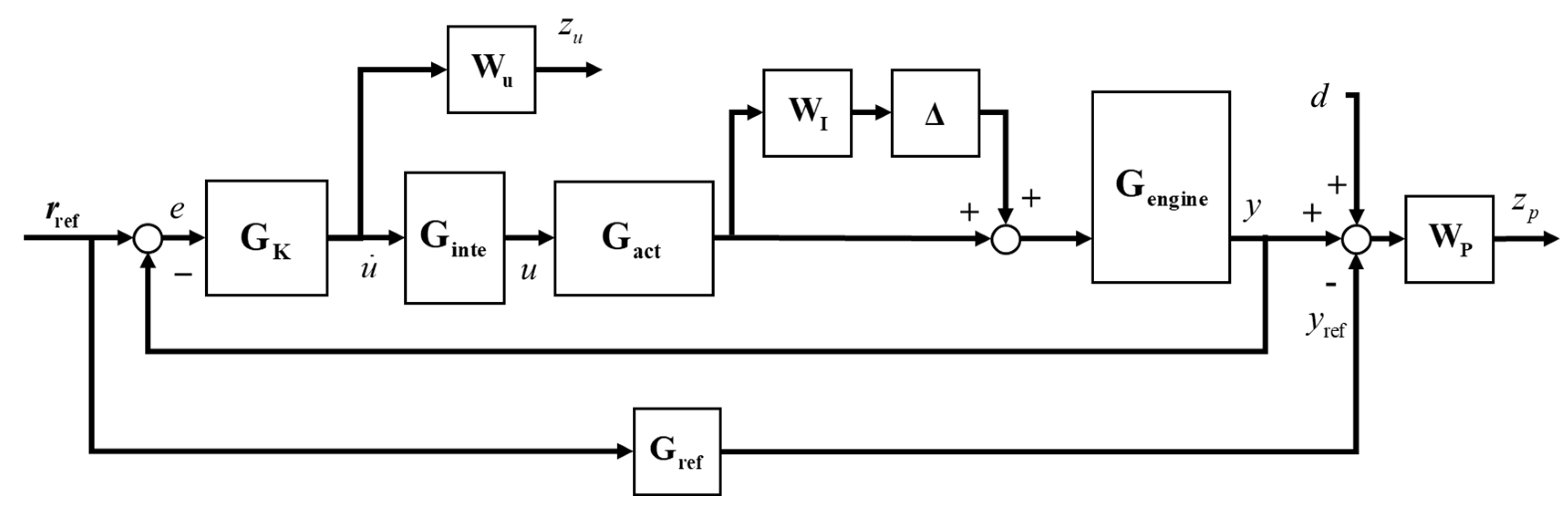
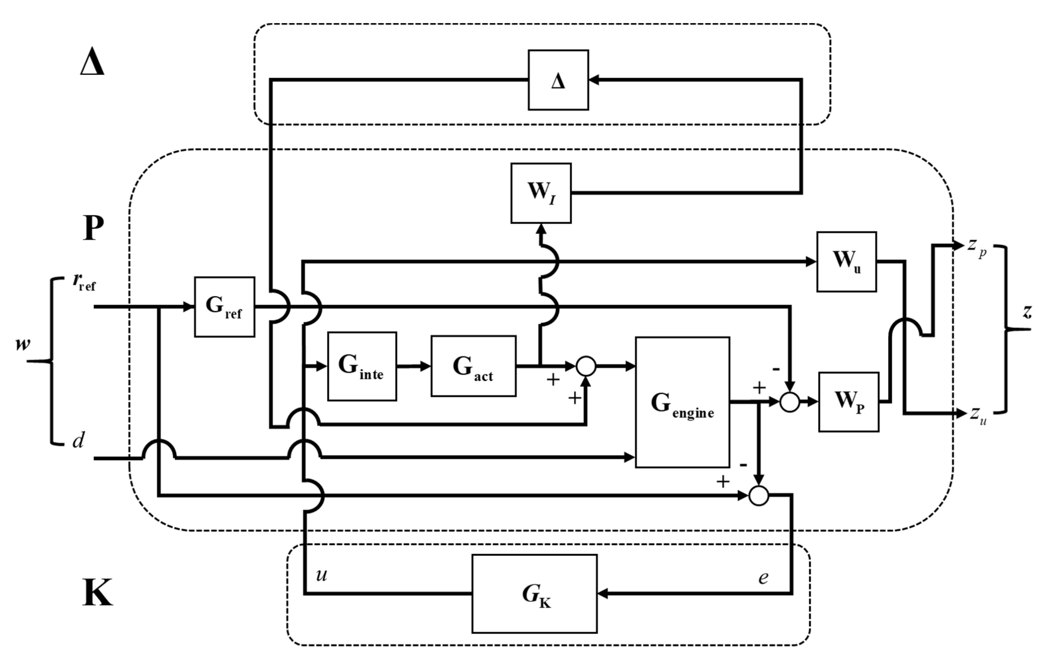
2.4. μ-Synthesis Control Design

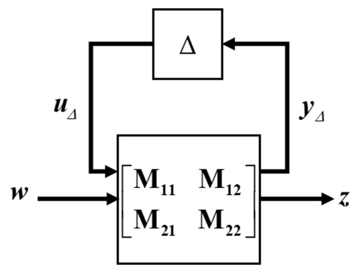
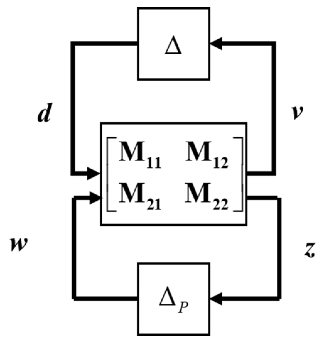
2.4.1. Robust Stability and Robust Performance

For the dual-loop control architecture in Figure 2, we define

$$G_{\mathrm{act}}=\left[\begin{array}{cc}{G}_{W_{\mathrm{f}}}& 0\\ 0& G_{A_8}\end{array}\right],G_{\mathrm{inte}}=\left[\begin{array}{cc}{G}_{W_{\mathrm{f}},\mathrm{inte}}& 0\\ 0& G_{A_8,\mathrm{inte}}\end{array}\right]$$

(48)

A weighted function frequency domain shaping model following the μ-synthesis control structure is proposed, as shown in Figure 3.

In the figure, $G_{\mathrm{ref}}$ represents the reference model transfer function matrix, $W_u$ is the weighting function matrix for controlling output energy suppression, $W_P$ is the weighting function matrix for tracking model error sensitivity, $\Delta$ is the unstructured uncertainty matrix with an ${\mathrm{H}}_{\infty }$ norm of at most 1, and $W_I$ is the weighting function matrix for the upper boundary of the uncertainty. $r_{\mathrm{ref}}={\left[\begin{array}{cc}{r}_{F_{\mathrm{N}}}& r_{{\pi }_{\mathrm{T}}}\end{array}\right]}^{\mathrm{T}}$ is the reference command vector, $u={\left[\begin{array}{cc}{u}_{W_{\mathrm{f}}}& u_{A_8}\end{array}\right]}^{\mathrm{T}}$ is the controller output vector, $z={\left[\begin{array}{cc}{z}_p& z_u\end{array}\right]}^{\mathrm{T}}$ is the performance evaluation vector, $y={\left[\begin{array}{cc}{F}_{\mathrm{N}}& {\pi }_{\mathrm{T}}\end{array}\right]}^{\mathrm{T}}$ is the engine measurement output vector, $y_{\mathrm{ref}}={\left[\begin{array}{cc}{F}_{\mathrm{N},\mathrm{ref}}& {\pi }_{\mathrm{T},\mathrm{ref}}\end{array}\right]}^{\mathrm{T}}$ is the reference model output vector, and $d={\left[\begin{array}{cc}{d}_{F_{\mathrm{N}}}& d_{{\pi }_{\mathrm{T}}}\end{array}\right]}^{\mathrm{T}}$ is the external disturbance input vector.

The closed-loop system with uncertainty depicted in Figure 3 is transformed equivalently into a μ-synthesis standard $\Delta$-P-K framework structure, illustrated in Figure 4.

The expression for the $\Delta$-P-K control system is as follows:

$$\left[\begin{array}{c}{y}_{\Delta }\\ z\\ y_K\end{array}\right]=\left[\begin{array}{ccc}{P}_{11}\left(s\right)& P_{12}\left(s\right)& P_{13}\left(s\right)\\ P_{21}\left(s\right)& P_{22}\left(s\right)& P_{23}\left(s\right)\\ P_{31}\left(s\right)& P_{32}\left(s\right)& P_{33}\left(s\right)\end{array}\right]\left[\begin{array}{c}{u}_{\Delta }\\ w\\ u_K\end{array}\right]$$

(49)

$$u_{\Delta }=\Delta \left(s\right)\cdot y_{\Delta }$$

(50)

$$u_K=K\left(s\right)\cdot y_K$$

(51)

Performing a low fractional transformation on $P(s)$ and $G_{\mathrm{K}}(s)$, the constructed $M(s)$ is as follows:

$$\begin{array}{l}M(s)=F_l(P(s),G_{\mathrm{K}}(s))\\ \hspace{1em}\hspace{1em}=\left[\begin{array}{cc}{M}_{11}\left(\mathrm{s}\right)& M_{12}\left(\mathrm{s}\right)\\ M_{21}\left(\mathrm{s}\right)& M_{22}\left(\mathrm{s}\right)\end{array}\right]=\left[\begin{array}{cc}{P}_{11}\left(\mathrm{s}\right)& P_{12}\left(\mathrm{s}\right)\\ P_{21}\left(\mathrm{s}\right)& P_{22}\left(\mathrm{s}\right)\end{array}\right]+\left[\begin{array}{c}{P}_{13}\left(\mathrm{s}\right)\\ P_{23}\left(\mathrm{s}\right)\end{array}\right]G_{\mathrm{K}}\left(\mathrm{s}\right){\left[I-P_{33}\left(\mathrm{s}\right)G_{\mathrm{K}}\left(\mathrm{s}\right)\right]}^{-1}\left[\begin{array}{cc}{P}_{31}\left(\mathrm{s}\right)& P_{32}\left(\mathrm{s}\right)\end{array}\right]\end{array}$$

(52)

Then

$$\left[\begin{array}{c}{y}_{\Delta }\\ z\end{array}\right]=\left[\begin{array}{cc}{M}_{11}(s)& M_{12}(s)\\ M_{21}(s)& M_{22}(s)\end{array}\right]\left[\begin{array}{c}{u}_{\Delta }\\ \omega \end{array}\right]$$

(53)

Equation (53) can be represented by Figure 5.

The closed-loop stability of the $\Delta -M$ system under the perturbation of uncertainty $\Delta$ is measured by $\overline{\sigma }(\Delta )$, which is

$$\mu (M)={\displaystyle \frac{1}{\underset{\Delta }{\min }\left\{\overline{\sigma }(\Delta )|\det (I-M\Delta )=0, \mathrm{for} \mathrm{structured} \Delta \right\}}}$$

(54)

Thus, a quantitative μ-test method for robust stability under uncertainty is provided. If both $M(s)$ and $\Delta$ are stable, the system is robustly stable for all allowable uncertainties when $\overline{\sigma }(\Delta (j\omega ))<1,\forall \omega$, if and only if

$$\mu (M(j\omega ))<1,\hspace{1em}\forall \omega$$

(55)

By embedding the performance uncertainty matrix ${\Delta }_P$ into the $\Delta -M$ system, the extended uncertainty matrix is defined:

$$\widehat{\Delta }=\left[\begin{array}{cc}\Delta & 0\\ 0& {\Delta }_P\end{array}\right]$$

(56)

Thus, the $\widehat{\Delta }-M$ control system is constructed, as shown in Figure 6.

A quantitative μ-test method for the robust performance of the extended uncertainty $\widehat{\Delta }$ is given. For the $\widehat{\Delta }-M$ system, where $M$ is internally stable and satisfies

$$\begin{array}{c}{\Vert F\Vert }_{\infty }={\Vert F_u(M,\widehat{\Delta })\Vert }_{\infty }={\Vert M_{22}\left(s\right)+M_{21}\left(s\right)\widehat{\Delta }\left(s\right){\left[I-M_{11}\left(s\right)\widehat{\Delta }\left(s\right)\right]}^{-1}{M}_{12}\left(s\right)\Vert }_{\infty }<1\\ \forall \widehat{\Delta },{\Vert \widehat{\Delta }\Vert }_{\infty }<1\end{array}$$

(57)

if and only if

$${\mu }_{\widehat{\Delta }}(M(j\omega ))<1,\forall \omega$$

(58)

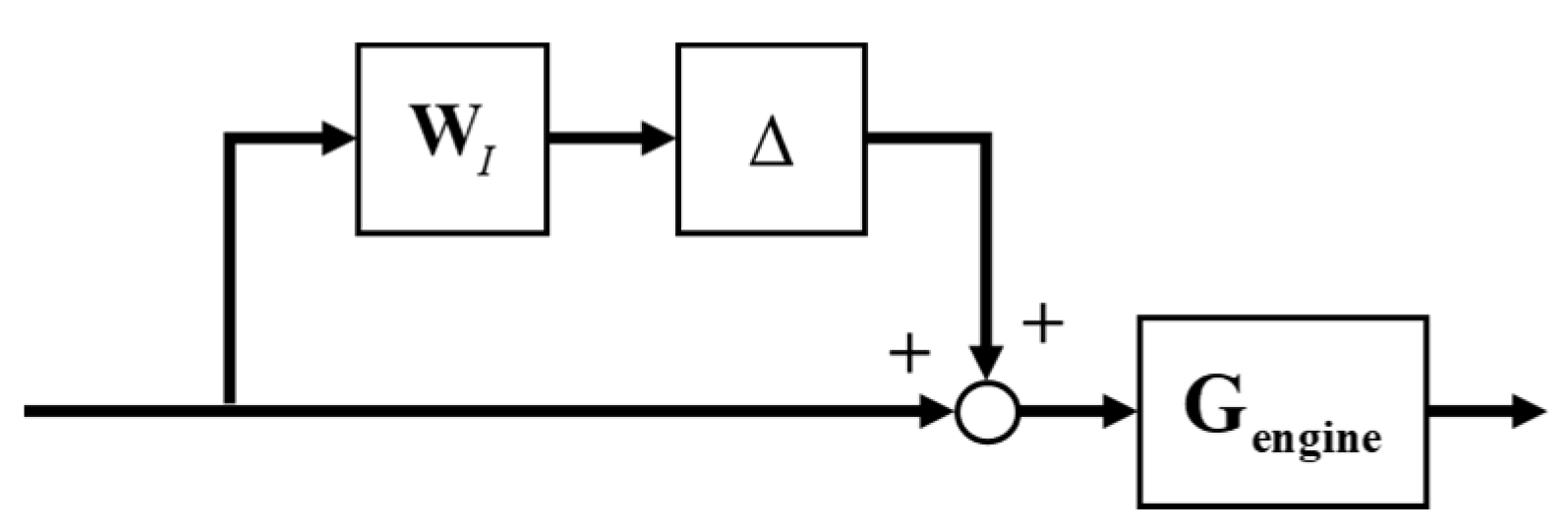
2.4.2. Weighted Function Frequency Domain Shaping Design

When the engine operates at non-design points, its dynamic characteristics deviate, and the resulting uncertainty can be characterized by multiplicative uncertainty, as shown in Figure 7. In the figure, $W_I$ represents the uncertainty weighting function, and $\Delta$ represents arbitrary non-structural uncertainty, satisfying ${\Vert \Delta \Vert }_{\infty }<1$.

Let $r{u}_0$ denote the steady-state relative uncertainty, ${\omega }_I$ represent the frequency at which the relative uncertainty reaches 100%, and $r{u}_{\infty }$ be the amplitude of the weight function at high frequencies. Then, $W_I$ can be expressed as the following minimum-phase rational function:

$$W_I(s)={\displaystyle \frac{\frac{s}{{\omega }_I}+r{u}_0}{\frac{s}{r{u}_{\infty }{\omega }_I}+1}}$$

(59)

For good model tracking servo performance in the low-frequency range and effective suppression of low-frequency disturbances, $W_P$ is designed:

$$W_P(s)={\displaystyle \frac{\alpha }{{\epsilon }_P}}{\displaystyle \frac{\frac{s}{{\omega }_P}+1}{\frac{s}{{\omega }_P{\epsilon }_P}+1}}, (0.1<\alpha \le 1,0<{\epsilon }_S<<1)$$

(60)

where $\alpha$ and ${\epsilon }_P$ are the weighting function performance adjustment factors, and ${\omega }_P$ is the closed-loop system bandwidth.

To suppress control output saturation, $W_u$ is designed as follows:

$$W_u(s)=\gamma {\displaystyle \frac{\frac{s}{{\omega }_u}+1}{\frac{s}{\left({\omega }_u/{\epsilon }_u\right)}+1}}$$

(61)

where $\gamma$, ${\omega }_u$, and ${\epsilon }_u$ are control energy suppression adjustment factors.

Once the weighting functions are established, they are used in the D–K iteration algorithm [22] to compute the dual-loop μ-synthesis controller.

3. Design Example

3.1. Plant Description and Controller Design

According to Section 2.1, the normalized linear model for the small bypass ratio turbofan engine design point is given by

$$\begin{array}{l}A=\left[\begin{array}{cc}-6.44& 5.62\\ 0.30& -3.74\end{array}\right],B=\left[\begin{array}{cc}0.48& 2.09\\ 0.66& -0.012\end{array}\right]\\ C=\left[\begin{array}{cc}1.77& 0.042\\ -0.87& 1.13\end{array}\right],D=\left[\begin{array}{cc}0.38& -0.70\\ 7.5\times {10}^{-4}& 0.74\end{array}\right]\end{array}$$

The parameters at the design point are as follows:

$$\begin{array}{cccc}PLA={65}^{\circ }& dPs=0 \mathrm{kPa}& dTs=0 \mathrm{K}& \\ H=0 \mathrm{km}& Ma=0& W_{\mathrm{f}}=1.144 \mathrm{kg}/\mathrm{s}& A_8=0.2984{ \mathrm{m}}^2\\ N_1=10080 \mathrm{rpm}& N_2=12910 \mathrm{rpm}& F_{\mathrm{N}}=51071.22 \mathrm{N}& {\pi }_{\mathrm{T}}=8.701\\ T_4=1664.18 \mathrm{K}& SMFD=13.93 \%& SMFC=18.23 \%& SMC=30.51 \%\end{array}$$

PLA stands for throttle angle, SMFD represents the surge margin for the fan outer duct, SMFC is the surge margin for the fan inner duct, and SMC refers to the surge margin for the compressor.

The given equivalent transfer function for the dual-loop actuator is

$$G_{\mathrm{act}}=\left[\begin{array}{cc}{\displaystyle \frac{1}{0.16s+1}}& 0\\ 0& {\displaystyle \frac{1}{0.14s+1}}\end{array}\right]$$

The augmented controlled plant is

$$G_{\mathrm{Aug}}=\left[\begin{array}{cc}{\displaystyle \frac{2.336(s^2+12.47s+48.41)}{s (s+6.96) (s+6.078) (s+3.216)}}& {\displaystyle \frac{-5.1578 (s+0.6457) (s+4.245)}{s (s+6.96) (s+7.359) (s+3.216)}}\\ {\displaystyle \frac{0.0045646 (s+453.8) (s+0.6065)}{s (s+6.96) (s+6.078) (s+3.216)}}& {\displaystyle \frac{5.4506 (s+4.695) (s+3.007)}{s (s+6.96) (s+7.359) (s+3.216)}}\end{array}\right]$$

According to the thrust estimation algorithm mentioned in Section 2.3, the maximum thrust estimation error compared to the nonlinear model thrust is within 0.013%. The corresponding comparison curves can be seen in the subsequent simulation result plots.

Let the model uncertainty exist at low, mid, and high frequency ranges with uncertainties of 10%, 100%, and 1000%, respectively. The uncertainty weighting function mentioned in Section 2.4.2 is

$$W_I=\left[\begin{array}{cc}{\displaystyle \frac{10s+20}{s+200}}& 0\\ 0& {\displaystyle \frac{10s+20}{s+200}}\end{array}\right]$$

Design performance sensitivity function tuning parameters are $\alpha =0.6, {\epsilon }_P={10}^{-6}, {\omega }_P=3 \mathrm{rad}/\mathrm{s}$, then

$$W_P(s)=\left[\begin{array}{cc}{\displaystyle \frac{1.8s+5.4}{3s+9\times {10}^{-6}}}& 0\\ 0& {\displaystyle \frac{1.8s+5.4}{3s+9\times {10}^{-6}}}\end{array}\right]$$

The designed control energy suppression adjustment factors are $\gamma =0.01, {\omega }_u=20 \mathrm{rad}/\mathrm{s}, {\epsilon }_u=0.002$, then

$$W_u\left(s\right)=\left[\begin{array}{cc}{\displaystyle \frac{100s+2000}{20s+200000}}& 0\\ 0& {\displaystyle \frac{100s+2000}{20s+200000}}\end{array}\right]$$

We design the reference model as

$$G_{\mathrm{ref}}(s)=\left[\begin{array}{cc}{\displaystyle \frac{25}{\left(s^2+9s+25\right)}}& 0\\ 0& {\displaystyle \frac{25}{\left(s^2+9s+25\right)}}\end{array}\right]$$

Using the D–K iteration method [27], an 18th-order μ-synthesis controller based on the analysis of Section 2.4.1 is obtained.

The singular value curves ${\mu }_{\Delta }(M(j\omega ))$ and ${\mu }_{\widehat{\Delta }}(M(j\omega ))$ in the closed-loop system are shown in Figure 8.

Figure 8a shows that $\sup {\mu }_{\Delta }(M(j\omega ))<1$, indicating that the closed-loop system is robustly stable. Figure 8b shows that $\sup {\mu }_{\widehat{\Delta }}(M(j\omega ))<1$, indicating that the closed-loop system has robust performance.

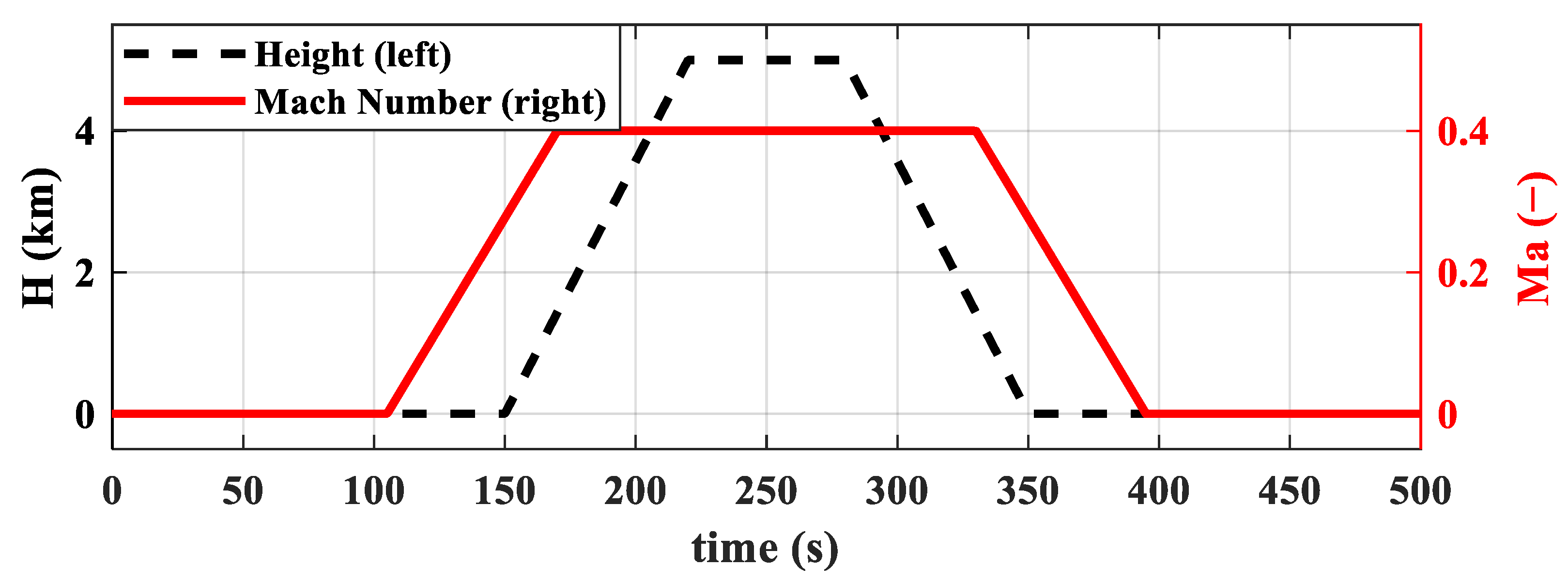
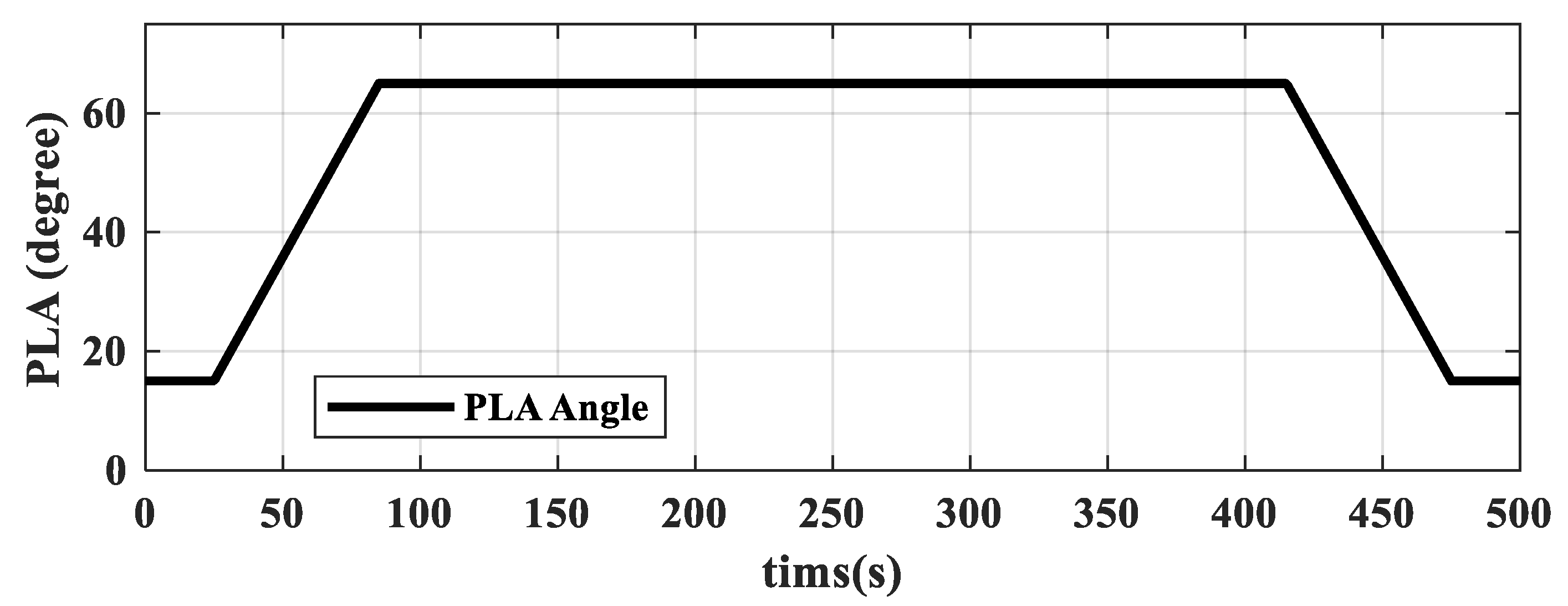
3.2. Simulation Test Procedure

Next, nonlinear simulation verification of the designed μ-synthesis controller is performed. The trajectory of flight altitude and flight Mach number is shown in Figure 9.

The simulation lasts 500 s. Altitude H stays at 0 km from 0 to 150 s, ascends at 0.07 km/s from 150 to 220 s, stays at 5 km from 220 to 280 s, descends at −0.07 km/s from 280 to 350 s, and remains at 0 km from 350 to 500 s.

From 0 to 105 s, the flight Mach number (Ma) remains at 0. From 105 to 170 s, Ma increases at 0.0062 per second. From 170 to 330 s, Ma stays at 0.4. From 330 to 395 s, Ma decreases at 0.0062 per second. From 395 to 500 s, Ma remains at 0.

The curve of PLA variation is shown in Figure 10. It stays at 15° from 0 s to 25 s (idle state), gradually increases to 65° (military power) from 25 s to 85 s, remains at 65° from 85 s to 415 s, gradually decreases to 15° from 415 s to 475 s, and stays at 15° from 475 s to 500 s.

3.3. Closed-Loop Simulation Results

The closed-loop system is constructed according to the structure shown in Figure 2 and closed-loop simulations are carried out with the parameters and input conditions shown in Section 3.1.

Thrust command, thrust estimation, and thrust response curves are shown in Figure 11. The three lines are closely matched with a maximum steady-state error below 0.1%. The results show that the estimated thrust maintains high accuracy within the flight envelope. Additionally, the designed μ-synthesis multivariable controller ensures precise servo tracking of the thrust command despite disturbances from changing flight conditions.

The comparison of the ${\pi }_{\mathrm{T}}$ response and command is in Figure 12. It can be seen that the ${\pi }_{\mathrm{T}}$ command and response match well, with a maximum steady-state error below 0.13%. Combined with the results of Figure 11, the designed μ-synthesis controller ensures servo tracking and decoupled control of thrust and turbine pressure ratio under varying flight conditions. This implies that the engine can maintain relatively stable operating points while meeting thrust requirements, thus avoiding dangerous conditions.

The fuel flow rate and nozzle throat area curve are shown in Figure 13.

The turbine inlet temperature ($T_4$) response curve is shown in Figure 14. The result shows that the $T_4$ is always (except the model initialization phase) below the limited temperature of 1800 K. This means that under the control of this μ-synthesis controller, it can satisfy the servo tracking of thrust and turbine drop pressure ratio while ensuring that the hot components do not exceed limiting temperature, which prolongs its service life. In addition, the application of the thrust estimation algorithm in Section 2.3 can also be used to estimate other unmeasurable parameters such as $T_4$ and the surge margin, etc. It can also be seen from the results in Figure 14 that the estimated value of $T_4$ matches well with the calculated one from the nonlinear model, which further proves the effectiveness of the estimation algorithm.

The fan bypass surge margin response curve is shown in Figure 15, with a minimum surge margin of 8.1% of the fan bypass, which is no less than the set limited surge margin.

The fan core surge margin response curve is shown in Figure 16, and it can be observed that the minimum surge margin of the fan core is 8.7%, staying above the limit line throughout the simulation.

The high-pressure compressor surge margin response curve is shown in Figure 17.

The minimum surge margin of the high-pressure compressor is 22.9%, as shown in Figure 18a. Surge margins of the fan and compressor are also estimated by applying the thrust estimation algorithm, and it can be seen from Figure 15, Figure 16 and Figure 17 that the estimated values of the three surge margins are consistent with the values calculated by the nonlinear model and do not fall below the set minimum surge margin boundaries during the simulation process.

High-pressure rotor speed and low-pressure rotor speed responses are shown in Figure 18b. Neither the high- nor low-pressure rotor speeds of the engine within the flight envelope exceeded the maximum physical speed of the limitations, ensuring mechanical integrity.

Figure 14, Figure 15, Figure 16, Figure 17 and Figure 18 demonstrate that employing the μ-synthesis controller ensures that the closed-loop system maintains thrust servo tracking performance without encountering issues such as over-temperature, over-speed, or surging.

4. Discussion

For the direct thrust control requirements, a dual-loop multivariable direct thrust control method is proposed for turbofan engines. The conclusions drawn through nonlinear system simulations are as follows:

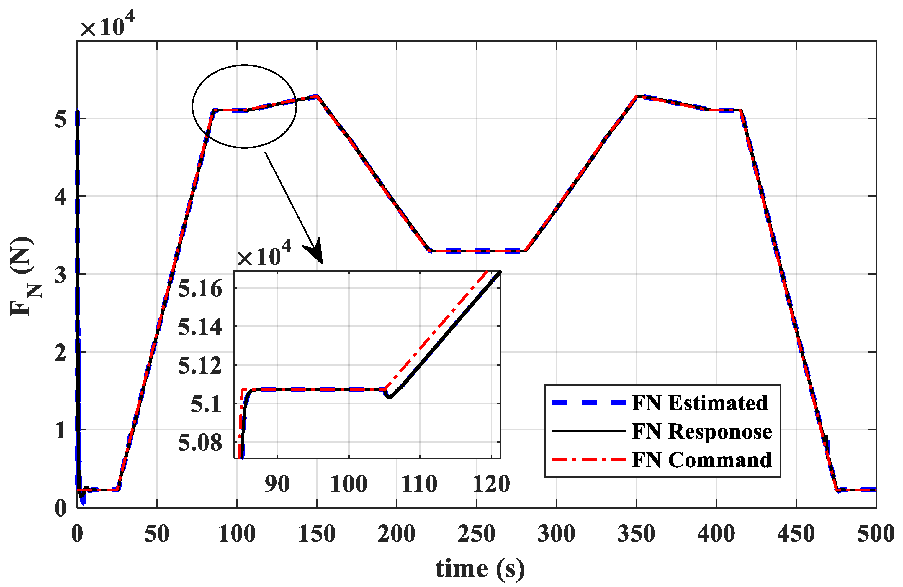
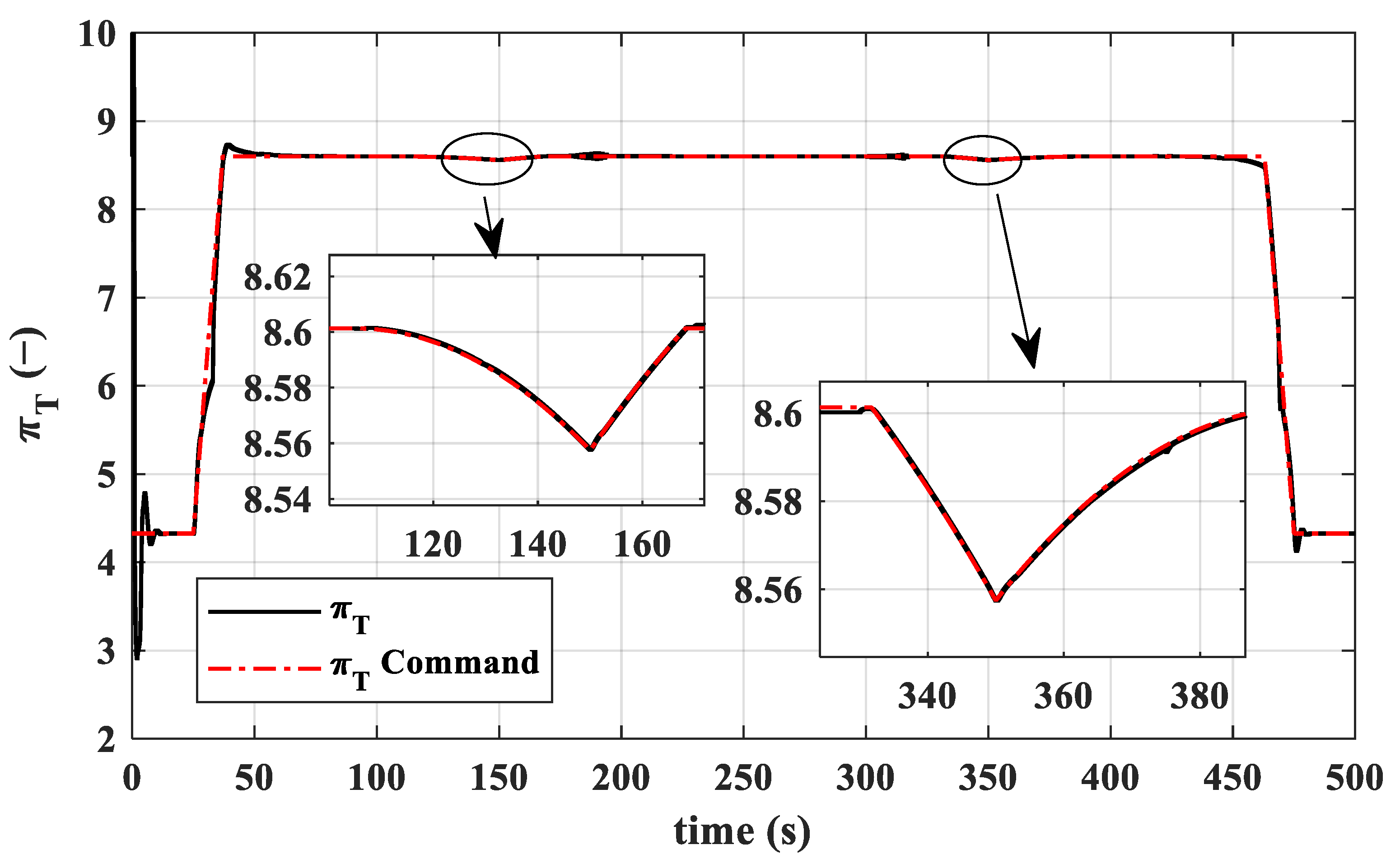
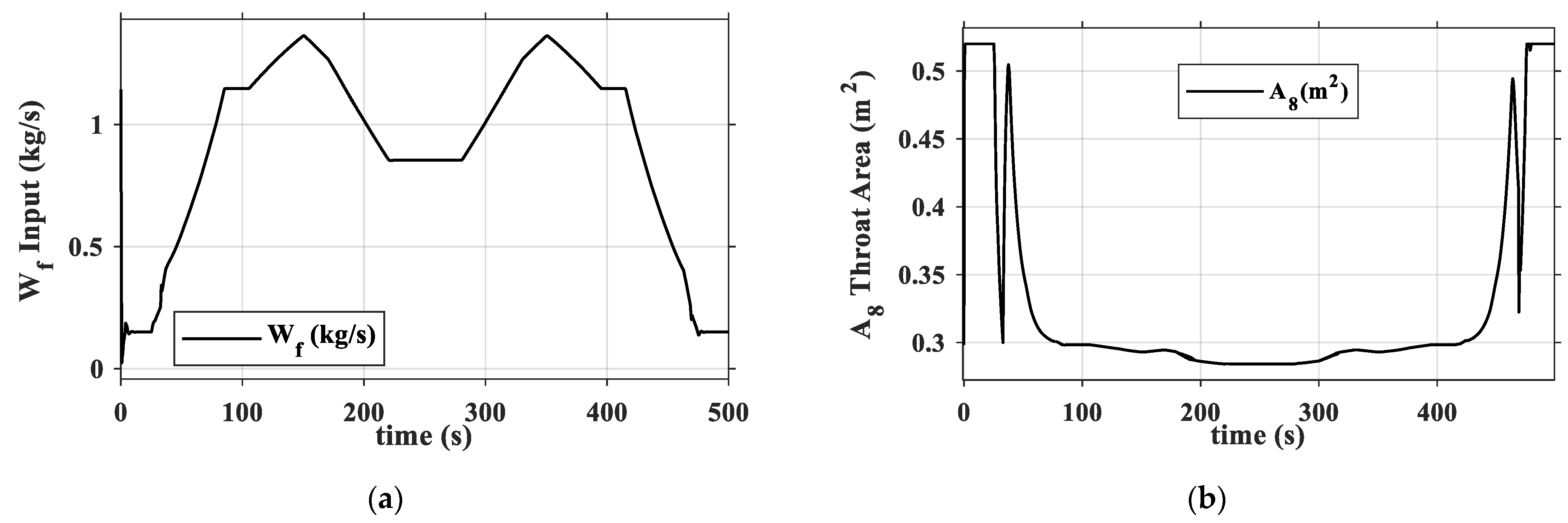
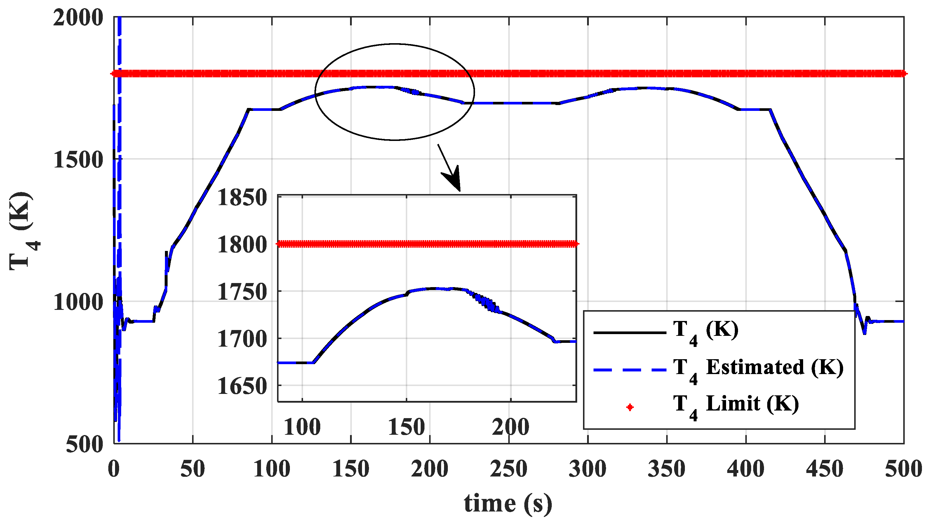
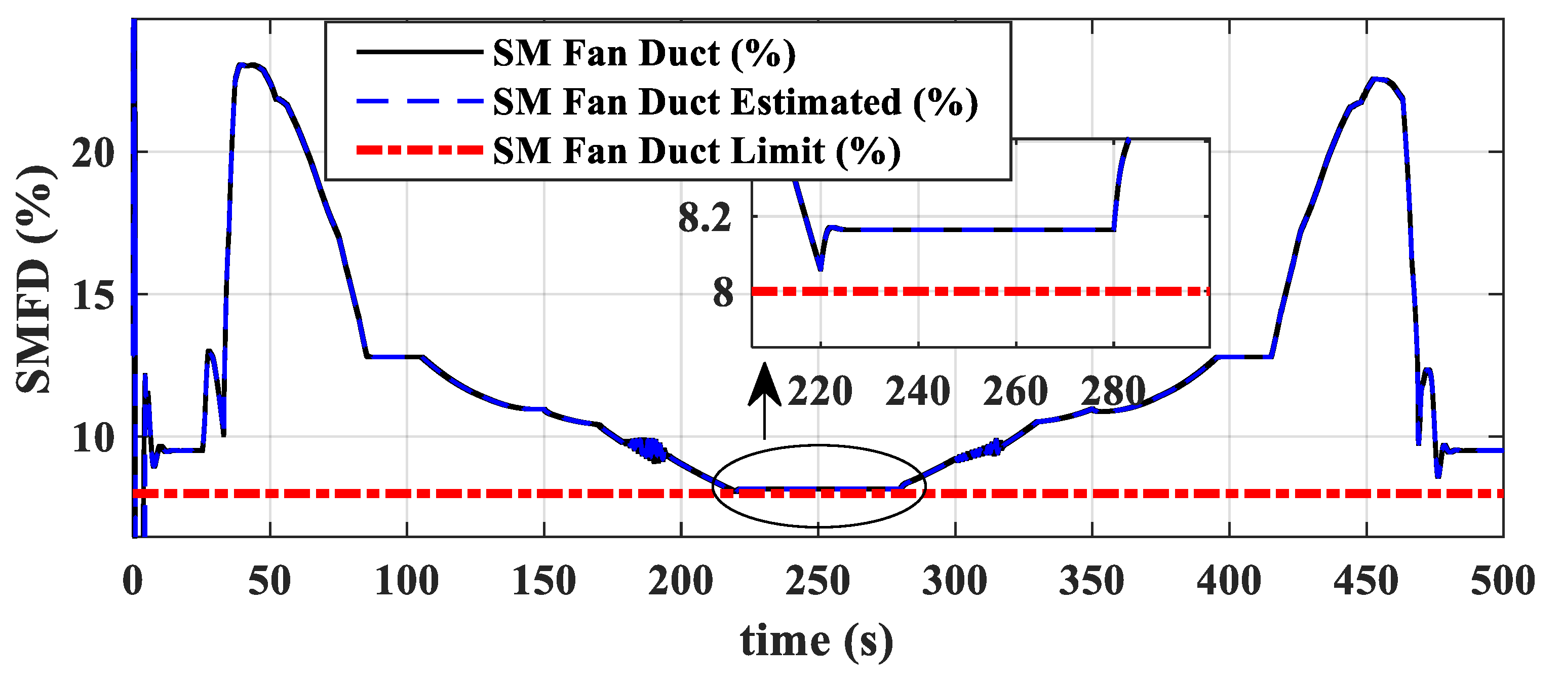
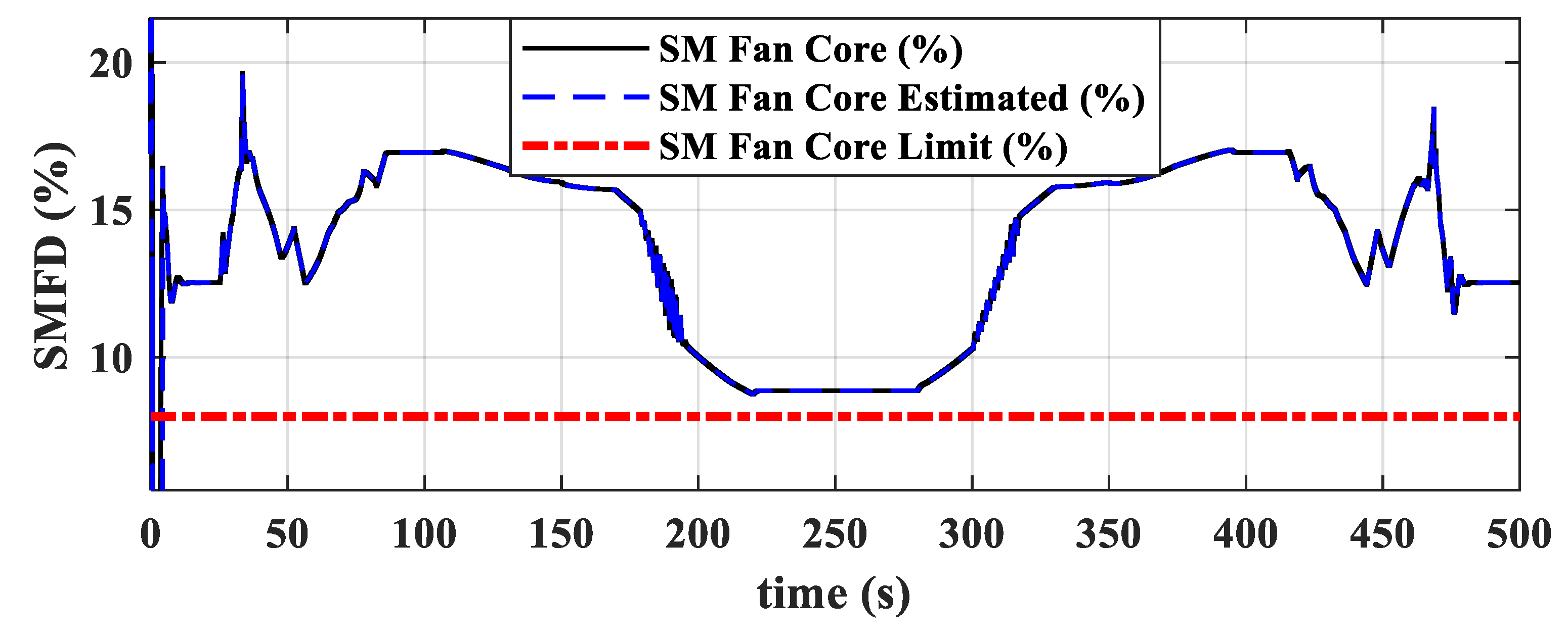
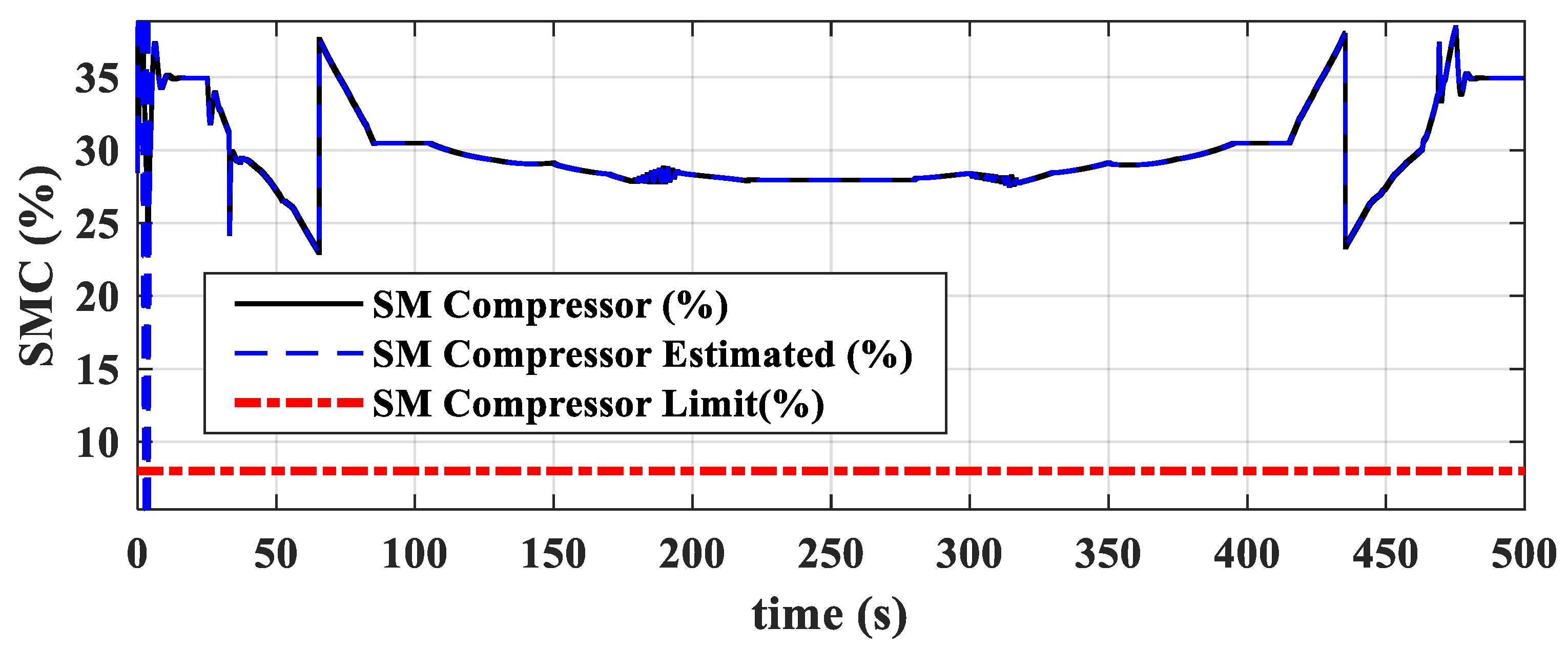
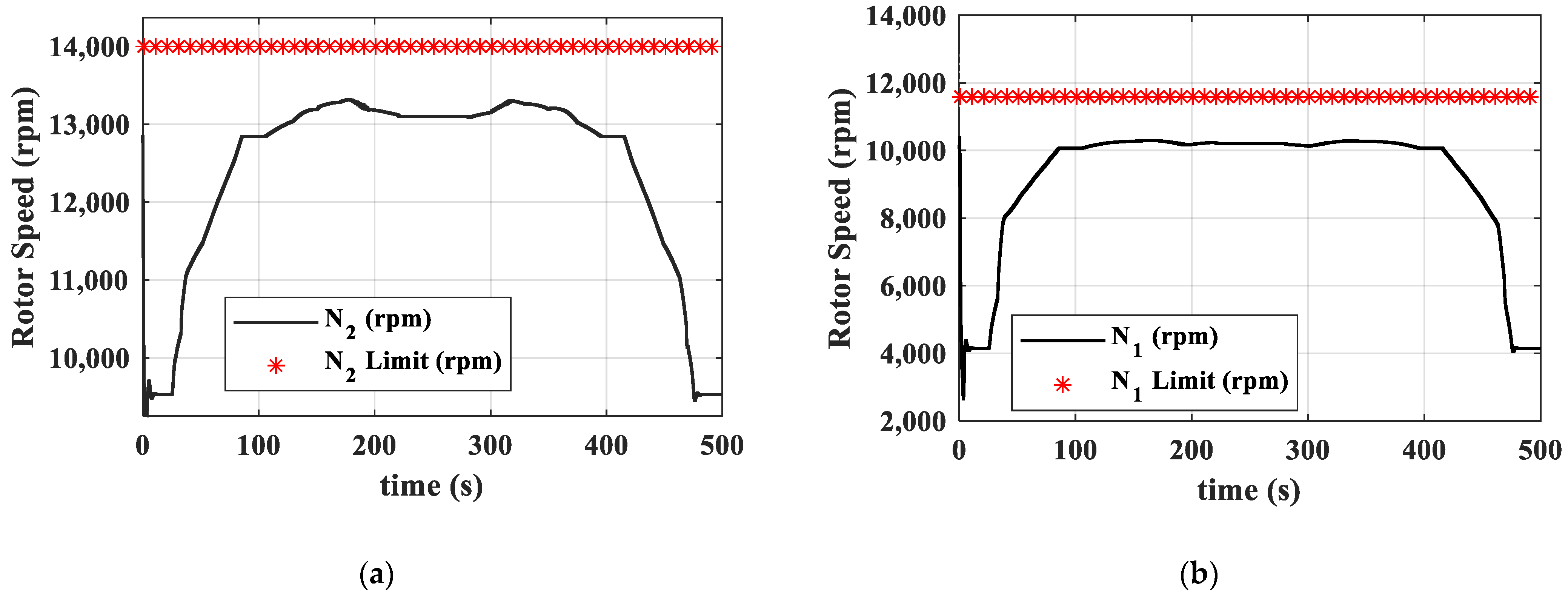
• During external disturbances and changes in flight conditions, this dual-loop control scheme, which uses fuel flow to control thrust and nozzle area to control turbine pressure ratio, effectively ensures thrust command tracking while guaranteeing no overheat ($T_4<1800 \mathrm{K}$), surge ($SMFD>8\%$, $SMFC>8\%$, and $SMC>8\%$), or overspeed ($N_1<11592 \mathrm{rpm}$, $N_2<14000 \mathrm{rpm}$).
• Compared to the nonlinear model, the proposed thrust estimation algorithm is both fast and accurate, with a maximum relative error in thrust estimation of no more than 0.013%.
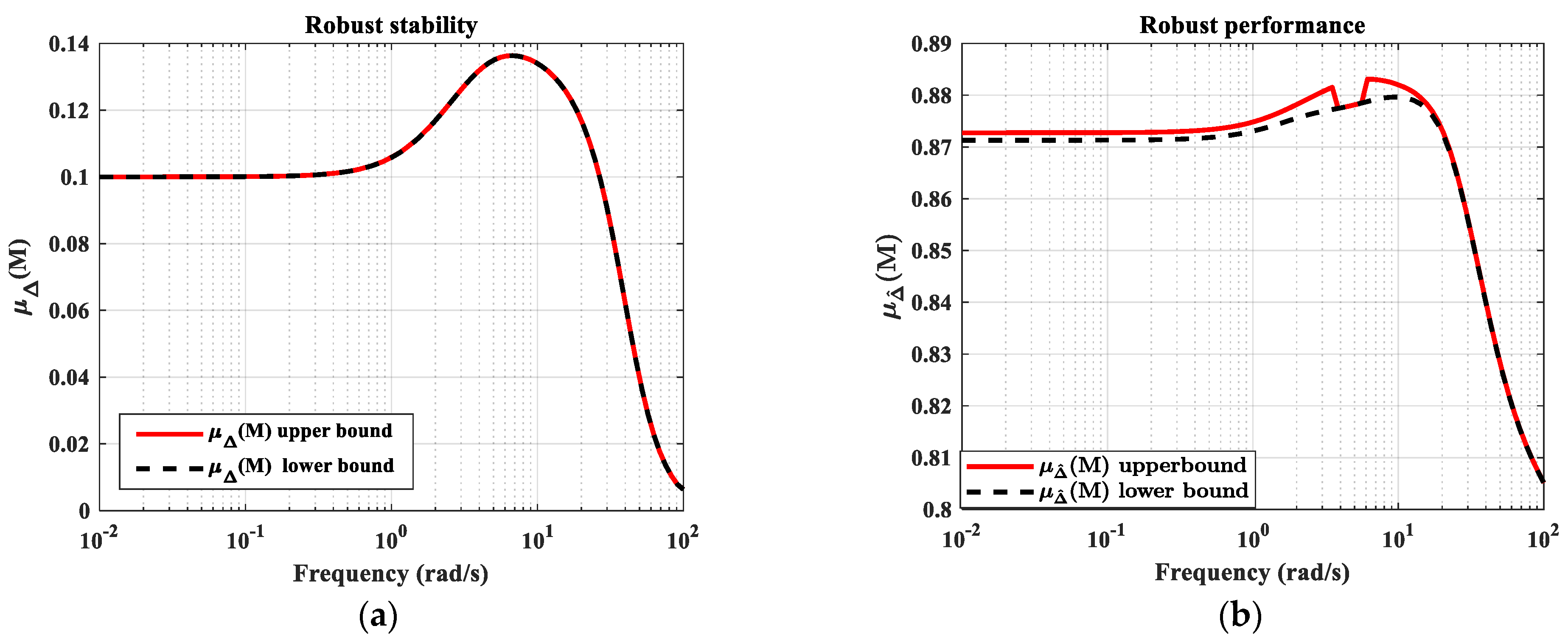
• Within the specified flight envelope, the dual-loop direct thrust μ-synthesis control achieves both servo performance and anti-disturbance capabilities for direct thrust control, with a maximum steady-state thrust relative error of less than 0.1%. The designed μ-synthesis controller demonstrates robust stability and performance within the uncertainty range, both stability and performance indicators below 1.

In the future, the subsequent research should consider adding control variables such as the guide vane angle to realize the control of the surge margin, as well as realizing the fusion of the steady state and transition state without switching control through the μ-synthesis method.

References

1. Dennis, C.; Sanjay, G.; Hiller, S.-J.; Horn, W.; Kumar, A.; Mathews, H.K.; Moustapha, H.; Pfoertner, H.; Rosenfeld, T.; Rybarik, P.; et al. More Intelligent Gas Turbine Engines; North Atlantic Treaty Organisation: Brussels, Belgium, 2009; ISBN 978-92-837-0080-7. [Google Scholar]
2. Hanz, R. Advanced Control of Turbofan Engines; Springer: New York, NY, USA, 2011; ISBN 978-1-4614-1171-0. [Google Scholar]
3. Wang, X.; Yang, S.-B.; Zhu, M.-Y.; Kong, X.-X. Aeroengine Control Principles; Science Press: Beijing, China, 2021; ISBN 978-7-03-069605-2. [Google Scholar]
4. Jack, D.M.; William, H.H.; David, T.P. Aircraft Engine Design, 2nd ed.; AIAA: Reston, VA, ISA, 2002; ISBN 978-1-56347-538-2. [Google Scholar]
5. Zhao, H.; Liao, Z.; Liu, J.; Li, M.; Liu, W.; Wang, L.; Song, Z. A Highly Robust Thrust Estimation Method with Dissimilar Redundancy Framework for Gas Turbine Engine. Energy 2022, 245, 123255. [Google Scholar] [CrossRef]
6. Wei, Z.; Zhang, S.; Jafari, S.; Nikolaidis, T. Gas Turbine Aero-Engines Real Time on-Board Modelling: A Review, Research Challenges, and Exploring the Future. Prog. Aerosp. Sci. 2020, 121, 100693. [Google Scholar] [CrossRef]
7. Litt, J.S. An Optimal Orthogonal Decomposition Method for Kalman Filter-Based Turbofan Engine Thrust Estimation. J. Eng. Gas Turbine Power 2007, 130, 011601. [Google Scholar] [CrossRef]
8. Litt, J.S.; Sowers, T.S.; Corporation, A.; Garg, S. A Retro-Fit Control Architecture to Maintain Engine Performance with Usage. In Proceedings of the 18th ISABE Conference, Beijing, China, 2–7 September 2007. [Google Scholar]
9. Lu, F.; Gao, T.; Huang, J.; Qiu, X. A Novel Distributed Extended Kalman Filter for Aircraft Engine Gas-Path Health Estimation with Sensor Fusion Uncertainty. Aerosp. Sci. Technol. 2019, 84, 90–106. [Google Scholar] [CrossRef]
10. Lu, F.; Li, Z.; Huang, J.; Jia, M. Hybrid State Estimation for Aircraft Engine Anomaly Detection and Fault Accommodation. AIAA J. 2020, 58, 1748–1762. [Google Scholar] [CrossRef]
11. Villarreal-Valderrama, F.; Santana Delgado, C.; Zambrano-Robledo, P.D.C.; Amezquita-Brooks, L. Turbojet Direct-Thrust Control Scheme for Full-Envelope Fuel Consumption Minimization. Aircr. Eng. Aerosp. Technol. 2020, 93, 437–447. [Google Scholar] [CrossRef]
12. Sheng, H.; Zhang, T. Aircraft Engine Thrust Estimator Design Based on GSA-LSSVM. Int. J. Turbo Jet Engines 2017, 34, 279–285. [Google Scholar] [CrossRef]
13. Su, W.; Zhao, Y.; Sun, J. Novel Weighted Least Squares Support Vector Regression for Thrust Estimation on Performance Deterioration of Aero-Engine. Trans. Nanjing Univ. Aeronaut. Astronaut. 2012, 29, 25–32. [Google Scholar]
14. Baklacioglu, T. Metaheuristic and Machine Learning Models for TFE-731-2, PW4056, and JT8D-9 Cruise Thrust. Int. J. Turbo Jet Engines 2017, 34, 221–232. [Google Scholar] [CrossRef]
15. Zhao, Y.-P.; Hu, Q.-K.; Xu, J.-G.; Li, B.; Huang, G.; Pan, Y.-T. A Robust Extreme Learning Machine for Modeling a Small-Scale Turbojet Engine. Appl. Energy 2018, 218, 22–35. [Google Scholar] [CrossRef]
16. Song, H.-Q.; Li, B.-W.; Zhu, F.-X. Research on Aero-Engine Thrust Estimate Based on Extreme Learning Machine. In Proceedings of the 2016 IEEE Advanced Information Management, Communicates, Electronic and Automation Control Conference (IMCEC), Xi’an, China, 3–5 October 2017; pp. 1170–1174. [Google Scholar]
17. Zhao, Y.-P.; Li, Z.-Q.; Hu, Q.-K. A Size-Transferring Radial Basis Function Network for Aero-Engine Thrust Estimation. Eng. Appl. Artif. Intell. 2020, 87, 103253. [Google Scholar] [CrossRef]
18. Li, Z.-Q.; Zhao, Y.-P.; Cai, Z.-Y.; Xi, P.-P.; Pan, Y.-T.; Huang, G.; Zhang, T.-H. A Proposed Self-Organizing Radial Basis Function Network for Aero-Engine Thrust Estimation. Aerosp. Sci. Technol. 2019, 87, 167–177. [Google Scholar] [CrossRef]
19. Wang, B.; Xu, J.; Liu, X.; Zheng, Q. Thrust Estimation for Aero-Engine Based on Deep Convolution Neural Network. IOP Conf. Ser. Mater. Sci. Eng. 2020, 752, 012009. [Google Scholar] [CrossRef]
20. Zhao, Y.-P.; Chen, Y.-B.; Li, Z.-Q. A Proposed Algorithm Based on Long Short-Term Memory Network and Gradient Boosting for Aeroengine Thrust Estimation on Transition State. Proc. Inst. Mech. Eng. Part G J. Aerosp. Eng. 2021, 235, 2182–2192. [Google Scholar] [CrossRef]
21. Wang, B. Intelligent Direct Thrust Control of Turbofan Engines based on Mathematical Dynamic Models. Ph.D. Thesis, Beihang University, Beijing, China, 2014. [Google Scholar]
22. Zheng, Q.; Miao, L.; Zhang, H.; Ye, Z. On-Board Real-Time Optimization Control for Turbofan Engine Thrust under Flight Emergency Condition. Proc. Inst. Mech. Eng. Part J. Syst. Control Eng. 2017, 231, 554–566. [Google Scholar] [CrossRef]
23. Zheng, Q.; Pang, S.; Zhang, H.; Hu, Z. A Study on Aero-Engine Direct Thrust Control with Nonlinear Model Predictive Control Based on Deep Neural Network. Int. J. Aeronaut. Space Sci. 2019, 20, 933–939. [Google Scholar] [CrossRef]
24. Zheng, Q.; Du, Z.; Fu, D.; Hu, Z.; Zhang, H. Direct Thrust Inverse Control of Aero-Engine Based on Deep Neural Network. Int. J. Turbo Jet-Engines 2021, 38, 391–396. [Google Scholar] [CrossRef]
25. Jin, C.; Zheng, Q.; Zhang, H.; Fang, J.; Hu, Z. Direct Thrust Predictive Control of Aeroengine Based on Compact Propulsion System Dynamic Model-State Variable Model. J. Propuls. Technol. 2022, 43, 354–363. [Google Scholar] [CrossRef]
26. Zhu, Y.; Huang, J.; Pan, M.; Zhou, W. Direct Thrust Control for Multivariable Turbofan Engine Based on Affine Linear Parameter-Varying Approach. Chin. J. Aeronaut. 2022, 35, 125–136. [Google Scholar] [CrossRef]
27. Liu, J.; Wang, X.; Liu, X.; Zhu, M.; Pei, X.; Dan, Z.; Zhang, S. μ-Synthesis-based Robust L1 Adaptive Control for Aeropropulsion System Test Facility. Aerosp. Sci. Technol. 2023, 140, 108457. [Google Scholar] [CrossRef]
28. Gu, D.-W.; Petkov, P.H.; Konstantinov, M.M. Robust Control Design with MATLAB®; Advanced Textbooks in Control and Signal Processing; Springer: London, UK, 2013; ISBN 978-1-4471-4681-0. [Google Scholar]
29. Liu, J.; Wang, X.; Zhu, M.; Miao, K. Multi-Variable Adaptive Control Method for Turbofan Engine with Dynamic and Input Uncertainties. J. Eng. Gas Turbine Power 2021, 143, 071027. [Google Scholar] [CrossRef]
30. Shi, Y.; Zhao, J. Supervisory Control of Multiple Switching Laws with Performance Guidance for Aeroengines. IEEE Trans. Control Syst. Technol. 2019, 27, 2557–2564. [Google Scholar] [CrossRef]
31. Xiao, L. Aeroengine Multivariable Nonlinear Tracking Control Based on Uncertainty and Disturbance Estimator. J. Eng. Gas Turbine Power 2014, 136, 121601. [Google Scholar] [CrossRef]
32. Liu, J.; Wang, X.; Liu, X.; Pei, X.; Dan, Z.; Zhang, S.; Yang, S.; Zhang, L. An Anti-windup Design with Local Sector and H2/H Optimization for Flight Environment Simulation System. Aerosp. Sci. Technol. 2022, 128, 107787. [Google Scholar] [CrossRef]
33. Liu, J.; Wang, X.; Liu, X.; Zhu, M.; Pei, X.; Zhang, S.; Dan, Z. μ-Synthesis Control with Reference Model for Aeropropulsion System Test Facility Under Dynamic Coupling and Uncertainty. Chin. J. Aeronaut. 2023, 36, 246–261. [Google Scholar] [CrossRef]
34. Wang, H.; Guo, Y.; Lu, J.; Li, G. Research of aero-engine two degrees-of-freedom robust controller based on linear matrix inequality approach. J. Aerosp. Power 2009, 24, 1413–1419. [Google Scholar] [CrossRef]
Figure 1. Schematic diagram and cross-section definition of the engine.
Symmetry 16 00944 g001
Figure 2. Scheme of direct thrust dual-loop control system.
Symmetry 16 00944 g002
Figure 3. Model following the μ-synthesis control structure based on weight function frequency domain shaping.
Symmetry 16 00944 g003
Figure 4. μ-synthesis standard Δ -P-K framework.
Symmetry 16 00944 g004
Figure 5. Control system with uncertainty described by Δ M .
Symmetry 16 00944 g005
Figure 6. Standard architecture for robust performance analysis.
Symmetry 16 00944 g006
Figure 7. Input multiplicative uncertainty structure.
Symmetry 16 00944 g007
Figure 8. The robust stability and robust performance of the closed-loop system. (a) Robust stability curve: μ Δ ( M ( j ω ) ) ; (b) robust performance curve: μ Δ ^ ( M ( j ω ) ) .
Symmetry 16 00944 g008
Figure 9. Flight height and Ma input versus time.
Symmetry 16 00944 g009
Figure 10. PLA input of the controller.
Symmetry 16 00944 g010
Figure 11. Engine thrust command, feedback signal, and thrust estimation response to external input variations.
Symmetry 16 00944 g011
Figure 12. Engine turbine pressure ratio ( π T ) command and feedback signal variation curve with external inputs.
Symmetry 16 00944 g012
Figure 13. Fuel flow rate and nozzle throat area response curve with input conditions. (a) W f input of the engine. (b) A 8 input of the engine.
Symmetry 16 00944 g013
Figure 14. Response curves of turbine inlet temperature ( T 4 ) and estimation with respect to input conditions.
Symmetry 16 00944 g014
Figure 15. Response curves of the fan bypass surge margin (SMFD) and its estimated value with respect to the variation of input conditions.
Symmetry 16 00944 g015
Figure 16. Response curves of the fan core surge margin (SMFC) and its estimated value with respect to the variation of input conditions.
Symmetry 16 00944 g016
Figure 17. Response curves of the high-pressure compressor surge margin (SMC) and its estimated value with respect to the variation of input conditions.
Symmetry 16 00944 g017
Figure 18. Response curves of the engine rotor speeds. (a) High-pressure rotor speed response. (b) Low-pressure rotor speed response.
Symmetry 16 00944 g018
Disclaimer/Publisher’s Note: The statements, opinions and data contained in all publications are solely those of the individual author(s) and contributor(s) and not of MDPI and/or the editor(s). MDPI and/or the editor(s) disclaim responsibility for any injury to people or property resulting from any ideas, methods, instructions or products referred to in the content.