The Closed-Form Solutions of an SIS Epidemic Reaction–Diffusion Model with Advection in a One-Dimensional Space Domain

Abstract

This work investigates a class of susceptible–infected–susceptible (SIS) epidemic model with reaction–diffusion–advection (RDA) by utilizing the Lie group methods. The Lie symmetries are computed for the three widely used incidence functions: standard incidence, mass action incidence, and saturated incidence. The Lie algebra for the SIS-RDA epidemic model is four-dimensional for the standard incidence function, three-dimensional for mass action incidence, and two-dimensional for saturated incidence. The reductions and closed-form solutions for the SIS-RDA epidemic model for the standard incidence infection mechanism are established. The transmission dynamics of an infectious disease utilizing closed-form solutions is presented. To illustrate the paths of susceptible and infected populations, we consider the Cauchy problem. Moreover, a sensitivity analysis is conducted to provide insights into potential policy recommendations for disease control.

1. Introduction

A susceptible–infected–susceptible (SIS) compartmental model is governed by a system of $2\times 2$ ordinary differential equations (ODEs). When the spatial movements of both infected and susceptible populations are taken into account, the phenomena are governed by a system of $2\times 2$ reaction–diffusion-type partial differential equations (PDEs). Allen et al. [1], following suggestions from two papers by Fitzgibbon et al. [2,3], introduced an SIS reaction–diffusion model for an epidemic in a continuous spatial habitat. Peng and Liu [4], focused on the global stability of the steady states within an SIS epidemic reaction–diffusion model. Veliov [5] focused on a class of SIS epidemic models in a heterogeneous population. Gudelj et al. [6] investigated how spatial movement and group interactions influence the dynamics of disease spread in social animals using an SIS-type framework for two classes of two social groups.

The biased and/or passive movement behavior can be incorporated into the SIS reaction–diffusion model by adding an advection term. In some realistic environments, populations may exhibit biased or passive movements in certain directions due to external stimuli such as water flow [7], wind [8], and so on. In this framework, several mathematical models have been introduced to understand the effects of migratory movement and spatial heterogeneity on disease transmission. These models are governed by a system of reaction–diffusion–advection (RDA)-type PDEs.

In [9,10], the SIS-RDA epidemic model for the infection mechanism with standard incidence was investigated. Cui et al. [11] analyzed the SIS-RDA model using mass action and standard rate. Zhang and Cu [12] investigated the SIS-RDA model for the saturated incidence. Ge et al. [13] examined an SIS-RDA epidemic model across different risk domains, providing valuable insights into disease dynamics. Similarly, Rao et al. [14] investigated an SIS epidemic model with a linear external source within a reaction–diffusion–advection framework, contributing to the understanding of disease spread in advective environments. We consider the following class of SIS-RDA system:

$$\left\{\begin{array}{cc}\hfill S_t& =\alpha S_{xx}-\theta S_x-\beta \Phi (S,I)+\gamma I,\hfill \\ \hfill I_t& =\alpha I_{xx}-\theta I_x+\beta \Phi (S,I)-\gamma I,\hfill \end{array}\right.$$

(1)

where the infection mechanism $\Phi =\Phi (S,I)$ is given by

$$\Phi (S,I)=\left\{\begin{array}{cc}\frac{SI}{S+I},\hfill & \mathrm{standard}\mathrm{incidence}\hfill \\ SI,\hfill & \mathrm{mass}\mathrm{action}\mathrm{incidence}\hfill \\ \frac{SI}{1+mI},\hfill & \mathrm{saturated}\mathrm{incidence}.\hfill \end{array}\right.$$

We denote the densities of susceptible and infected populations, with $S(t,x)$ and $I(t,x)$, respectively, at time t and at a location $x\in \mathbf{R}$. The constitutive parameter $\alpha$ denotes the diffusion coefficient for susceptible and infected populations, respectively. $\theta$ is the effective speed of the current (sometimes referred to as the advection speed/rate). It should be noted that $\theta$ must be non-negative, as x is defined to increase towards the downstream end. $\beta$ is the infection rate and $\gamma$ is the recovery/removed rate; both are positive constants.

In the first part of the article, we find the Lie symmetries for the SIS-RDA class represented by (1) for three widely used incidence functions. We apply the symmetry methods to find several reductions and closed-form solutions for SIS-RDA epidemic model (1) for the standard incidence function. It is worth mentioning here that non-linear models governed by a system of PDEs rarely exhibit closed-form solutions. Even if they exist, deriving these solutions is very challenging. Symmetry methods offer a methodological way to get a wide class of exact solutions. The classical books written on symmetry methods are [15,16,17,18,19,20,21,22]. Symmetry methods are effectively employed in several notable works, including [23,24,25,26,27]. Naz et al. [28,29] employed the symmetry methods to establish the closed-form solutions of the diffusive susceptible–infected–recovered (SIR) epidemic model. The book by Cheviakov and Zhao [30] provides a thorough exploration of nonlinear PDEs, delving into their characteristics, computational techniques, and diverse applications within PDE systems. For the computation of Lie symmetries, useful computer packages have been developed [31,32,33]. In the second part of the article, we solve the Cauchy problem for the SIS-RDA epidemic model for the standard incidence function, detailing the determination of arbitrary constants and the subsequent formulation and analysis of closed-form solutions. We show how the paths of susceptible and infected populations develop over time with parameter values taken from the existing literature. Furthermore, a sensitivity analysis is carried out to provide insights into potential policy recommendations for the control of the disease.

The layout of paper is as follows: the Lie symmetries for the SIS-RDA class represented by class (1) are derived in Section 2. Lie symmetries are established for the standard incidence function, mass action incidence function, and the saturated incidence function. The Lie algebra for the SIS-RDA epidemic model is four-dimensional for the standard incidence function, three-dimensional for mass action incidence, and two-dimensional for saturated incidence. In Section 3, the SIS-RDA epidemic model for the standard incidence function is analyzed in detail. By utilizing the combination of the Lie symmetries, we obtain the reductions and closed-form solutions for the SIS-RDA epidemic model for the standard incidence function. Section 4 is devoted to analyzing the transmission dynamics of an infectious disease by utilizing the derived closed-form solutions. To illustrate the path of susceptible and infected populations, we consider the Cauchy problem. We use graphs to effectively explain the phenomena observed in the model, employing parameter values sourced from the literature. Moreover, we perform a sensitivity analysis in the same section to provide insights into potential policy recommendations for disease control. The concluding remarks are presented in Section 5.

2. Lie Symmetries for the Class (1)

In this section, we establish the Lie symmetries for the general class of SIS-RDA epidemic model (1) for different infection mechanisms. We consider the three widely used types of incidence functions: standard incidence, mass action incidence, and saturated incidence.

2.1. Symmetry Infinitesimal Operator

A symmetry infinitesimal operator for class (1) has the form

$$X=\tau (t,x,S,I){\partial }_t+\xi (t,x,S,I){\partial }_t+{\eta }^1(t,x,S,I){\partial }_S+{\eta }^2(t,x,S,I){\partial }_I,$$

(2)

where the infinitesimal coordinates ${\xi }^1$, ${\xi }^2$, ${\eta }^1$, and ${\eta }^2$ are derived from the following invariance conditions:

$$\left\{\begin{array}{c}{X}^{\left(2\right)}\left(-S_t+\alpha S_{xx}-\theta S_x-\beta \Phi (S,I)+\gamma I\right){|}_{\left(1\right)}=0,\hfill \\ \\ X^{\left(2\right)}\left(-I_t+\alpha I_{xx}-\theta I_x+\beta \Phi (S,I)-\gamma I\right){|}_{\left(1\right)}=0.\hfill \end{array}\right.$$

(3)

The operator $X^{\left(2\right)}$ is as follows:

$$\begin{array}{ccc}\hfill X^{\left(2\right)}& =& X+{\zeta }_t^1\frac{\partial }{{\partial }_{S_t}}+{\zeta }_x^1\frac{\partial }{{\partial }_{S_x}}+{\zeta }_{xx}^1\frac{\partial }{{\partial }_{S_{xx}}}+{\zeta }_t^2\frac{\partial }{{\partial }_{I_t}}+{\zeta }_x^2\frac{\partial }{{\partial }_{I_x}}+{\zeta }_{xx}^2\frac{\partial }{{\partial }_{I_{xx}}}.\hfill \end{array}$$

(4)

As usual, the expressions of the coordinates ${\zeta }_t^1$, ${\zeta }_x^1$, ${\zeta }_{xx}^1$, ${\zeta }_t^2$,…are written as (see, e.g., [15,16,17,18,19,20,21,22])

$$\begin{array}{ccc}\hfill {\zeta }_t^1& =\hfill & \hfill D_t\left({\eta }_1\right)-S_t{D}_t\left(\tau \right)-S_x{D}_t\left(\xi \right),\\ \hfill {\zeta }_x^1& =\hfill & \hfill D_x\left({\eta }_1\right)-S_t{D}_x\left(\tau \right)-S_x{D}_x\left(\xi \right),\\ \hfill {\zeta }_{xx}^1& =\hfill & \hfill D_x\left({\zeta }_x^1\right)-S_{xt}{D}_x\left(\tau \right)-S_{xx}{D}_x\left(\xi \right),\\ \hfill {\zeta }_t^2& =\hfill & \hfill D_t\left({\eta }_2\right)-I_t{D}_t\left(\tau \right)-I_x{D}_t\left(\xi \right),\\ \hfill {\zeta }_x^2& =\hfill & \hfill D_x\left({\eta }_2\right)-I_t{D}_x\left(\tau \right)-I_x{D}_x\left(\xi \right),\\ \hfill {\zeta }_{xx}^2& =\hfill & \hfill D_x\left({\zeta }_x^2\right)-I_{xt}{D}_x\left(\tau \right)-I_{xx}{D}_x\left(\xi \right),\end{array}$$

(5)

where the operators $D_x$, and $D_t$ are the total derivatives with respect to x and t, respectively.

2.2. Determing System

From (3), after some basic simplifications, we derive the following Lie symmetry determining equations:

$$\begin{array}{c}\hfill \begin{array}{c}\hfill {\tau }_x=0,{\tau }_S=0,{\tau }_I=0,{\xi }_S=0,{\xi }_I=0,\\ \hfill {\tau }_t-\alpha {\tau }_{xx}-2{\xi }_x+\theta {\tau }_x=0,\\ \hfill {\eta }_{SS}^1=0,{\eta }_{II}^1=0,{\eta }_{SI}^1=0,{\eta }_{xI}^1=0,\\ \hfill {\eta }_{SS}^2=0,{\eta }_{II}^2=0,{\eta }_{SI}^2=0,{\eta }_{xS}^2=0,\\ \hfill {\xi }_t-\theta {\xi }_x-\alpha {\xi }_{xx}+2\alpha {\eta }_{xI}^2=0,\\ \hfill {\xi }_t-\theta {\xi }_x-\alpha {\xi }_{xx}+2\alpha {\eta }_{xS}^1=0,\\ \hfill (\beta \Phi -\gamma I)({\eta }_S^1-{\eta }_I^1-2{\xi }_x)+\gamma {\eta }^2-\beta {\Phi }_S{\eta }^1-\beta {\Phi }_I{\eta }^2+\alpha {\eta }_{xx}^1-\theta {\eta }_x^1-{\eta }_t^1=0,\\ \hfill (\beta \Phi -\gamma I)({\eta }_S^2-{\eta }_I^2+2{\xi }_x)-\gamma {\eta }^2+\beta {\Phi }_S{\eta }^1+\beta {\Phi }_I{\eta }^2+\alpha {\eta }_{xx}^2-\theta {\eta }_x^2-{\eta }_t^2=0.\end{array}\end{array}$$

(6)

These equations enable us to determine the form of the infinitesimal components $\tau$, $\xi$, ${\eta }^1$, and ${\eta }^2$ associated with the different forms of the infection mechanism $\Phi (S,I)$. It is straightforward to find

$$\begin{array}{c}\hfill \begin{array}{c}\hfill \tau =g_1\left(t\right),\xi =\frac{x}{2}{g}_1^{\prime }\left(t\right)+g_2\left(t\right),\\ \hfill {\eta }^1=g_3\left(t\right)S+g_4\left(t\right)I-\frac{S}{4\alpha }\left(\frac{x^2}{2}{g}_1^{″}\left(t\right)-\theta x{g}_1^{\prime }\left(t\right)+2x{g}_2^{\prime }\left(t\right)\right)+G_1(t,x),\\ \hfill {\eta }^2=g_3\left(t\right)I+g_5\left(t\right)S-\frac{I}{4\alpha }\left(\frac{x^2}{2}{g}_1^{″}\left(t\right)-\theta x{g}_1^{\prime }\left(t\right)+2x{g}_2^{\prime }\left(t\right)\right)+G_2(t,x),\end{array}\end{array}$$

(7)

with constraints

$$\begin{array}{c}\hfill \begin{array}{c}\hfill (\beta \Phi -\gamma I)({\eta }_S^1-{\eta }_I^1-2{\xi }_x)+\gamma {\eta }^2-\beta {\Phi }_S{\eta }^1-\beta {\Phi }_I{\eta }^2+\alpha {\eta }_{xx}^1-\theta {\eta }_x^1-{\eta }_t^1=0,\\ \hfill (\beta \Phi -\gamma I)({\eta }_S^2-{\eta }_I^2+2{\xi }_x)-\gamma {\eta }^2+\beta {\Phi }_S{\eta }^1+\beta {\Phi }_I{\eta }^2+\alpha {\eta }_{xx}^2-\theta {\eta }_x^2-{\eta }_t^2=0.\end{array}\end{array}$$

(8)

It is worth noting that the Lie symmetries for a different incidence coefficient can be derived using Equation (8).

2.3. Lie Symmetries for the Standard Incidence

Consider the standard incidence function

$$\Phi (S,I)=\frac{SI}{S+I}.$$

(9)

Using this function in Equation (8), we arrive at the following infinitesimal components:

$$\begin{array}{c}\hfill \tau =a_1,\xi =a_2+2a_3\alpha t,\\ \hfill {\eta }^1=a_3(t\theta -x)S+a_{4}S,\\ \hfill {\eta }^2=a_3(t\theta -x)I+a_{4}I.\end{array}$$

(10)

The corresponding basis of generators of the four-dimensional Lie algebra for the SIS-RDA system (1) for the standard incidence function are

$$\begin{array}{c}\hfill \begin{array}{cc}& X_1={\partial }_t,\hfill \\ & X_2={\partial }_x,\hfill \\ & X_3=2\alpha t{\partial }_x+(t\theta -x)S{\partial }_S+(t\theta -x)I{\partial }_I,\hfill \\ & X_4=S{\partial }_S+I{\partial }_I.\hfill \end{array}\end{array}$$

(11)

2.4. Lie Symmetries for the Mass Action Incidence

The mass action incidence function is given by

$$\Phi (S,I)=SI.$$

(12)

Substituting this function in Equation (8) leads to the following:

$$\begin{array}{c}\hfill \tau =c_1+2c_3\beta t,\xi =c_2+c_3\beta (t\theta +x),\\ \hfill {\eta }^1=2c_3(\gamma -\beta S),{\eta }^2=-2c_3\beta I.\end{array}$$

(13)

For system (1) with the standard incidence function, the basis of generators of the three-dimensional Lie algebra consists of $X_1$, $X_2$, and

$$X_5=2\beta t{\partial }_t+\beta (t\theta +x){\partial }_x+2(\gamma -\beta S){\partial }_S-2\beta I{\partial }_I.$$

(14)

2.5. Lie Symmetries for Saturated Incidence

The saturated incidence function is given by

$$\Phi (S,I)=\frac{SI}{1+mI},$$

(15)

where $m>0$ is the saturation coefficient. We solve Equation (8) for saturated incidence (15) and arrive at the two-dimensional Lie algebra for system (1) consisting of $X_1$ and $X_2$ only.

3. Reductions and Closed-Form Solutions of the SIS-RDA Epidemic Model for the Standard Incidence Function

In this section, we provide the reductions of the SIS-RDA epidemic model, governed by a system of two second-order nonlinear PDEs, to a system of two nonlinear second-order ODEs by utilizing the most general Lie symmetry operator. We also establish the traveling wave solutions via the linear combination of Lie symmetries $X_1$ and $X_2$. Several closed-form solutions are obtained by employing a linear combination of Lie symmetries $X_2$, $X_3$, and $X_4$.

3.1. Reductions of SIS-RDA Epidemic Model to a System of ODEs

The SIS-RDA epidemic model (1) for the standard incidence function takes the following form [9,10,11]:

$$\left\{\begin{array}{c}\hfill S_t=\alpha S_{xx}-\theta S_x-\frac{\beta SI}{S+I}+\gamma I,\\ \hfill I_t=\alpha I_{xx}-\theta I_x+\frac{\beta SI}{S+I}-\gamma I.\end{array}\right.$$

(16)

From the most general symmetry operator

$$X=a_1{X}_1+a_2{X}_2+a_3{X}_3+a_4{X}_4$$

(17)

assuming $a_1\ne 0$, the invariant surface conditions yield the following invariant solutions:

$$\begin{array}{c}\hfill S(t,x)=G_1\left(\chi \right)e^{\frac{3(\theta a_{3}t-2a_{3}x+2a_4)a_{1}t+4\left(a_3{d}_{I}t+\frac{3}{4}{a}_2\right)a_3{t}^2}{6a_1^2}},\\ \hfill I(t,x)=G_2\left(\chi \right)e^{\frac{3(\theta a_{3}t-2a_{3}x+2a_4)a_{1}t+4\left(a_3{d}_{I}t+\frac{3}{4}{a}_2\right)a_3{t}^2}{6a_1^2}}.\end{array}$$

(18)

Here, $G_1\left(\chi \right)$ and $G_2\left(\chi \right)$ are sought as functions of the so called similarity variable

$$\chi =\frac{-a_3{d}_I{t}^2+a_{1}x-a_{2}t}{a_1},$$

and their forms will be determined by substituting (18) in (16) and solving the following ODE system

$$\left\{\begin{array}{c}\hfill -a_1{d}_I(G_1+G_2)G_1^{″}+(a_1\theta -a_2)(G_1+G_2)F_1^{\prime }+(-a_3\chi +a_4)G_1^2\\ \hfill +(a_1\beta -a_1\gamma -a_3\chi +a_4)G_1{G}_2-a_1\gamma G_2^2=0,\\ \hfill a_1{d}_I(G_1+G_2)G_2^{″}-(a_1\theta -a_2)(G_1+G_2)G_2^{\prime }+(-a_1\gamma +a_3\chi -a_4)G_2^2\\ \hfill +(a_1\beta -a_1\gamma +a_3\chi -a_4)G_1{G}_2=0.\end{array}\right.$$

(19)

In this manner, we map the solution search for (16) onto the solutions of the ODE system (19) described by $G_1\left(\chi \right)$ and $G_2\left(\chi \right)$.

It is worth noticing that we can obtain several reductions of the SIS-RDA epidemic model (16) by choosing one, two, or three of the constants $a_2,a_3,a_4$ as zero in the system of reduced second-order ODEs (19). Each specific set of constants $a_1,a_2,a_3,a_4$ characterizes a combination of Lie symmetries corresponding to a unique reduction. For example, by choosing $a_2=0$ in the system of the reduced second-order ODEs (19), we obtain the reductions via $X_1$, $X_3$, and $X_4$ that are not invariant to the space translations. By adjusting these constants, we expand the scope for reducing the original system, which comprises a system of two second-order PDEs (16) representing the SIS-RDA epidemic model, to a system of two second-order ODEs (19).

3.2. Travelling Waves via $X_1$ and $X_2$

The traveling wave-type solutions are invariant with respect to space–time translations admitted by all autonomous equations [34,35]. In our specific case, this translates to the following:

$$S=G_1\left(\chi \right),I=G_2\left(\chi \right),\chi =x-\frac{a_2}{a_1}t.$$

(20)

The following reduced system can be easily obtained in this case by setting $a_3=a_4=0$ in the ODE system (19):

$$\left\{\begin{array}{c}\hfill a_1{d}_I(G_1+G_2)G_1^{″}-(a_1\theta -a_2)(G_1+G_2)G_1^{\prime }-(a_1\beta -a_1\gamma )G_1{G}_2+a_1\gamma G_2^2=0,\\ \hfill a_1{d}_I(G_1+G_2)G_2^{″}-(a_1\theta -a_2)(G_1+G_2)F_2^{\prime }+(a_1\beta -a_1\gamma )G_1{G}_2-a_1\gamma G_2^2=0.\end{array}\right.$$

(21)

Special classes of solutions can be derived from (21) by specifying $a_1$ and $a_2$. When $\frac{a_2}{a_1}=\theta$, applying the usual linear combination yields

$$G_1=G_2+C_0\chi +C_1$$

(22)

where $C_0$ and $C_1$ are arbitrary constants and

$$\begin{array}{c}\hfill -d_I(2G_2+C_0\chi +C_1)G_2^{″}+(\beta -2\gamma )G_2^2+(\beta -\gamma )(C_0\chi +C_1)G_2=0,\\ \hfill d_I(2G_2+C_0\chi +C_1)G_2^{″}+(\beta -2\gamma )G_2^2+(\beta -\gamma )(C_0\chi +C_1)G_2=0.\end{array}$$

(23)

Equations (22) and (23) provide the final expressions for $G_1\left(\chi \right)$ and $G_2\left(\chi \right)$ as

$$\begin{array}{c}\hfill G_1\left(\chi \right)=\frac{\gamma }{2\gamma -\beta }(C_0\chi +C_1),\\ \hfill G_2\left(\chi \right)=\frac{\beta -\gamma }{2\gamma -\beta }(C_0\chi +C_1),\end{array}$$

(24)

provided $\frac{a_2}{a_1}=\theta$ and thus $\chi =x-\theta t$. The final form of traveling wave solutions for the susceptible population $S(t,x)$ and the infected population $I(t,x)$ of the SIS-RDA epidemic model (16) is as follows:

$$\begin{array}{c}\hfill \begin{array}{c}\hfill S(t,x)=\frac{\gamma }{2\gamma -\beta }\left(C_0(x-\theta t)+C_1\right),\\ \hfill I(t,x)=\frac{\beta -\gamma }{2\gamma -\beta }\left(C_0(x-\theta t)+C_1\right).\end{array}\end{array}$$

(25)

These types of waves are typical of the system as their traveling speed is the same of the advection speed; we could call them advection waves.

3.3. Closed-Form Solutions by Using $X_2,X_3,X_4$

Now, we derive the closed-form solutions for the SIS-RDA epidemic model (16) by using the linear combination of $X_2,X_3,X_4$. Here we get the linear combination of $X_2,X_3,X_4$ by putting $a_1=0$ in (17). A similar procedure is carried out as in the previous case to obtain $\chi =t$, and

$$\begin{array}{c}\hfill S(t,x)=F_1\left(t\right)e^{\frac{x\left(2a_3\theta t-a_{3}x+2a_4\right)}{2(2a_3\alpha t+a_2)}},\\ \hfill I(t,x)=F_2\left(t\right)e^{\frac{x\left(2a_3\theta t-a_{3}x+2a_4\right)}{2(2a_3\alpha t+a_2)}},\end{array}$$

(26)

while the reduced system is as below:

$$\left\{\begin{array}{l}4{\left(a_3\alpha t+\frac{1}{2}{a}_2\right)}^2{F}_1^{\prime }+[t\alpha ({\theta }^{2}t+2\alpha )a_3^2+a_2{a}_3\left({\theta }^{2}t+\alpha \right)\\ +a_2{a}_4\theta -a_4^2\alpha ]\frac{F_1^2}{F_1+F_2}-4[\left(\gamma \alpha t-\beta \alpha t-\frac{1}{2}\alpha -\frac{1}{4}{\theta }^{2}t\right)\alpha t{a}_3^2+\\ \left(-\frac{1}{4}{\theta }^{2}t-\frac{1}{4}\alpha +\gamma t\alpha -\beta t\alpha \right)a_2{a}_3+\frac{1}{4}{a}_4^2\alpha +\frac{1}{4}{a}_2\left(-\beta a_2+\gamma a_2-a_4\theta \right)]\frac{F_1{F}_2}{F_1+F_2}\\ -4\gamma {\left(a_3\alpha t+\frac{1}{2}{a}_2\right)}^2\frac{F_2^2}{F_1+F_2}=0,\\ \\ {\left(2a_3\alpha t+a_2\right)}^2{F}_2^{\prime }+[\left(4t\gamma \alpha +2\alpha +{\theta }^{2}t\right)\alpha t{a}_3^2-a_4^2\alpha +\\ \left(4t\gamma \alpha +{\theta }^{2}t+\alpha \right)a_2{a}_3+a_2\left(a_2\gamma +a_4\theta \right)]\frac{F_2^2}{F_1+F_2}\\ +[\left({\theta }^{2}t+2\alpha +4\gamma t\alpha -4\beta t\alpha \right)\alpha t{a}_3^2+\left(\alpha +4\gamma \alpha t-4\beta \alpha t+{\theta }^{2}t\right)a_2{a}_3\\ -a_4^2\alpha +a_2\left(\gamma a_2-\beta a_2+a_4\theta \right)]\frac{F_1{F}_2}{F_1+F_2}=0.\end{array}\right.$$

(27)

3.3.1. Closed-Form Solution for $a_3\ne 0$

The general solution of Equation (27) for $a_3\ne 0$ where $a_2$ and $a_4$ can be zero or non-zero is

$$\begin{array}{c}\hfill \begin{array}{c}\hfill F_1\left(t\right)=\frac{\left(e^{-(\beta -\gamma )t}{C}_1\beta -C_2\gamma \right)e^{-\frac{2a_3\alpha {\theta }^{2}t(2a_3\alpha t+a_2)+{(a_2\theta -2a_4\alpha )}^2}{8{\alpha }^2{a}_3(2a_3\alpha t+a_2)}}}{\sqrt{2a_3\alpha t+a_2}\left(e^{-(\beta -\gamma )t}{C}_1-C_2\right)C_2},\\ \hfill F_2\left(t\right)=\frac{(\gamma -\beta )e^{-\frac{2a_3\alpha {\theta }^{2}t(2a_3\alpha t+a_2)+{(a_2\theta -2a_4\alpha )}^2}{8{\alpha }^2{a}_3(2a_3\alpha t+a_2)}}}{\sqrt{2a_3\alpha t+a_2}\left(e^{-(\beta -\gamma )t}{C}_1-C_2\right)}.\end{array}\end{array}$$

(28)

Substituting $F_1\left(t\right)$ and $F_2\left(t\right)$ from (28) into (26), we obtain the final expressions for the closed-form solutions for the susceptible population $S(t,x)$ and the infected population $I(t,x)$ of the SIS-RDA epidemic model (16) as follows:

$$\begin{array}{c}\hfill S(t,x)=\frac{\left(e^{-(\beta -\gamma )t}{C}_1\beta -C_2\gamma \right)e^{-\frac{4{(\theta t-x)}^2{a}_3^2{\alpha }^2-8x{a}_3{a}_4{\alpha }^2+2a_2{a}_3{\theta }^2\alpha t+{(a_2\theta -2a_4\alpha )}^2}{8{\alpha }^2{a}_3\left(2a_3\alpha t+a_2\right)}}}{\sqrt{2a_3\alpha t+a_2}{C}_2\left(e^{-(\beta -\gamma )t}{C}_1-C_2\right)},\\ \hfill I(t,x)=\frac{(\gamma -\beta )e^{-\frac{4{(\theta t-x)}^2{a}_3^2{\alpha }^2-8x{a}_3{a}_4{\alpha }^2+2a_2{a}_3{\theta }^2\alpha t+{(a_2\theta -2a_4\alpha )}^2}{8{\alpha }^2{a}_3\left(2a_3\alpha t+a_2\right)}}}{\sqrt{2a_3\alpha t+a_2}\left(e^{-(\beta -\gamma )t}{C}_1-C_2\right)}.\end{array}$$

(29)

It is worth emphasizing that the closed-form solution of the diffusive SIS epidemic reaction–diffusion model (16), presented in Equation (29), provides the benchmark for deriving closed-form solutions using different combinations of Lie symmetries $X_2$, $X_3$, and $X_4$. More precisely, it corresponds to the closed-form solution achieved using the Lie symmetry $X_3$ when both $a_2$ and $a_4$ are set to zero. Furthermore, the closed-form solution (29) yields the solution which corresponds to the closed-form solution obtained through the combination of the Lie symmetries $X_2$ and $X_3$ when $a_4$ is set to zero. Similarly, the closed-form solution involving the combination of Lie symmetries $X_3$ and $X_4$ can be deduced by setting $a_2$ to zero.

3.3.2. Closed-Form Solution for $a_3=0$, $a_2\ne 0$

Equation (26) for the $a_3=0$, $a_2\ne 0$ case simplifies to

$$\begin{array}{c}\hfill S(t,x)=F_1\left(t\right)e^{\frac{a_4}{a_2}x},\\ \hfill I(t,x)=F_2\left(t\right)e^{\frac{a_4}{a_2}x},\end{array}$$

(30)

and the general solution of the system of ODEs (27) is

$$\begin{array}{c}\hfill F_1\left(t\right)=\frac{e^{-\frac{a_4(a_2\theta -a_4\alpha )t}{a_2^2}}\left(e^{-(\beta -\gamma )t}{C}_1\beta -C_2\gamma \right)}{C_2(e^{-(\beta -\gamma )t}{C}_1-C_2)},\\ \hfill F_2\left(t\right)=\frac{e^{-\frac{a_4(a_2\theta -a_4\alpha )t}{a_2^2}}(\gamma -\beta )}{e^{-(\beta -\gamma )t}{C}_1-C_2},\end{array}$$

(31)

where $a_4$ can be zero or non-zero.

The substitution of $F_1\left(t\right)$ and $F_2\left(t\right)$ from Equation (31) into Equation (30) yields the closed-form solutions for the susceptible population $S(t,x)$ and the infected population $I(t,x)$ of the SIS-RDA epidemic model (16) as follows:

$$\begin{array}{c}\hfill S(t,x)=\frac{e^{\frac{a_2{a}_4(x-\theta t)+a_4^2\alpha t}{a_2^2}}\left(e^{-(\beta -\gamma )t}{C}_1\beta -C_2\gamma \right)}{C_2(e^{-(\beta -\gamma )t}{C}_1-C_2)},\\ \hfill I(t,x)=\frac{e^{\frac{a_2{a}_4(x-\theta t)+a_4^2\alpha t}{a_2^2}}(\gamma -\beta )}{e^{-(\beta -\gamma )t}{C}_1-C_2}.\end{array}$$

(32)

It is worth emphasizing that the closed-form solution of the SIS-RDA epidemic model (16), presented in Equation (32), provides a solution via $X_2$ when we set constant $a_4=0$.

This completes the search for all closed-form solutions of the SIS-RDA epidemic model (16) via different combinations of Lie symmetries.

4. The Transmission Dynamics of an Infectious Disease Utilizing the Closed-Form Solutions

In this section, we find the closed-form solution for the SIS-RDA epidemic model satisfying Cauchy’s problem. Next, we explore the derived closed-form solution that satisfies Cauchy’s problem for a real-world scenario to analyze the transmission dynamics of an infectious disease. The closed-form solution is visually illustrated using parameter values from the literature. Sensitivity analysis is performed to examine the effect of changes in the diffusion coefficient and advection rate.

4.1. A Cauchy Problem

A Cauchy problem for system (16) in the domain $D\equiv [0,+\infty )\times [0,+\infty )$ is characterized as follows: The initial conditions are assumed to be

$$\left\{\begin{array}{c}\hfill S(0,x)=S_0\Omega \left(x\right),\\ \hfill I(0,x)=I_0\Omega \left(x\right),\\ \hfill x\in [0,+\infty )\end{array}\right.$$

(33)

where the scaling constants $I_0$ and $S_0$ represent the initial densities (at $t=0$) of susceptible and infected populations and $\Omega \left(x\right)$ describes the initial distributions of susceptible and infected populations across the spatial domain. Applying the initial conditions (33) to the group-invariant solution (30) yields

$$F_1\left(0\right)=S_0,F_2\left(0\right)=I_0,$$

(34)

and the following expression for the initial distributions of susceptible and infected populations $\Omega \left(x\right)$ across the domain:

$$\Omega \left(x\right)=e^{-\lambda x},\lambda >0.$$

(35)

It is straightforward to determine that we must choose $a_4=-\lambda$ and $a_2=1$, which means the linear combination of symmetries $X_2-\lambda X_4$ is used to construct this solution. Applying the initial conditions of (34) to the general solution for $F_1\left(t\right)$ and $F_2\left(t\right)$ provided in (31), we have

$$\begin{array}{c}\hfill \frac{\beta C_1-\gamma C_2}{C_2(C_1-C_2)}=S_0,\\ \hfill \frac{\gamma -\beta }{C_2(C_1-C_2)}=I_0,\end{array}$$

(36)

which yields

$$\begin{array}{c}\hfill C_1=\frac{(\gamma -\beta )S_0+\gamma I_0}{(S_0+I_0)I_0},\\ \hfill C_2=\frac{\beta }{S_0+I_0}.\end{array}$$

(37)

Substituting the value of constants $C_1$ and $C_2$ from Equation (37) into $F_1\left(t\right)$ and $F_2\left(t\right)$ provided in (31), we have

$$\begin{array}{c}\hfill F_1\left(t\right)=\frac{(S_0+I_0)\left(((\gamma -\beta )S_0+\gamma I_0)e^{-(\beta -\gamma )t}-\gamma I_0\right)e^{\lambda (\theta +\lambda \alpha )t}}{\left((\gamma -\beta )S_0+\gamma I_0\right)e^{-(\beta -\gamma )t}-\beta I_0},\\ \hfill F_2\left(t\right)=\frac{(\gamma -\beta )(S_0+I_0)I_0{e}^{\lambda (\theta +\lambda \alpha )t}}{\left((\gamma -\beta )S_0+\gamma I_0\right)e^{-(\beta -\gamma )t}-\beta I_0}.\end{array}$$

(38)

Substituting the values of $F_1\left(t\right)$ and $F_2\left(t\right)$ from (38) into (30), the final form of the group-invariant solution for $S(t,x)$ and $I(t,x)$ satisfying the Cauchy problem (33) is

$$\begin{array}{c}\hfill S(t,x)=\frac{(S_0+I_0)\left(((\gamma -\beta )S_0+\gamma I_0)e^{-(\beta -\gamma )t}-\gamma I_0\right)e^{\lambda (\theta +\lambda \alpha )t-\lambda x}}{\left((\gamma -\beta )S_0+\gamma I_0\right)e^{-(\beta -\gamma )t}-\beta I_0},\\ \hfill I(t,x)=\frac{(\gamma -\beta )(S_0+I_0)I_0{e}^{\lambda (\theta +\lambda \alpha )t-\lambda x}}{\left((\gamma -\beta )S_0+\gamma I_0\right)e^{-(\beta -\gamma )t}-\beta I_0}.\end{array}$$

(39)

4.2. Visualization of Closed-Form Solutions

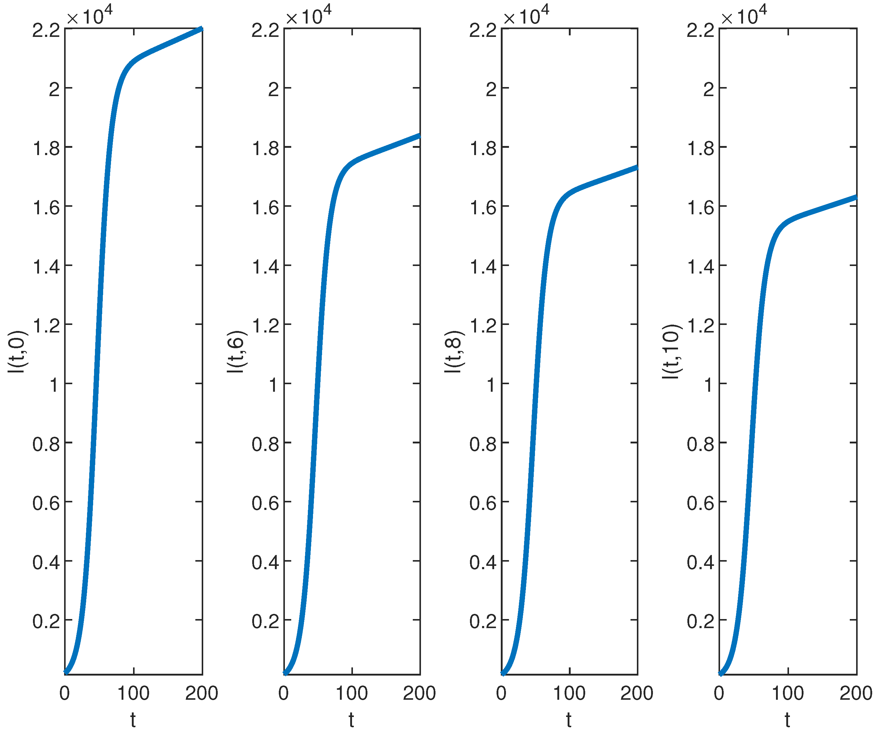
Next, we examine the closed-form solutions for the densities of a susceptible population S and infected population I as given in Equation (39). Specific parameter values sourced from the existing epidemiology literature (see, e.g., [28,29] and the references therein) are utilized. The selected benchmark values of parameter values are $S_0={10}^5-200$, $I_0=200$, $\lambda =0.03$, $\alpha =0.2$, $\beta =0.5$, $\gamma =0.4$, and $\theta =0.01$. We consider the spatial range $0\le x\le 10$ and the time interval $0\le t\le 200$ to visualize the closed-form solutions (39) graphically. Benchmark values play a vital role in numerical simulations for performing a sensitivity analysis for the epidemic models. All other parameters are set at the benchmark level while one or more parameters are changed to analyze their impact on the suspected and infected populations. It is important to mention here that the closed-form solution (39) can be rigorously tested across different parameter settings, not limited to those included here. The surface plots of the densities of the susceptible population $S(t,x)$ and infected population $I(t,x)$ are provided in Figure 1. The contour maps of the densities of susceptible and infected populations are provided in Figure 2. Figure 3 and Figure 4 present 2D plots showing susceptible and infected populations for the fixed values of $x=0,6,8,10$.

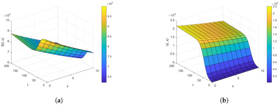
Figure 1. The density plot for (a) $S(t,x)$ and (b) $I(t,x)$ for $S_0={10}^5-200$, $I_0=200$, $\lambda =0.03$, $\alpha =0.2$, $\beta =0.5$, $\gamma =0.4$, and $\theta =0.01$ over the time intervals $0\le t\le 200$ and $0\le x\le 10$.

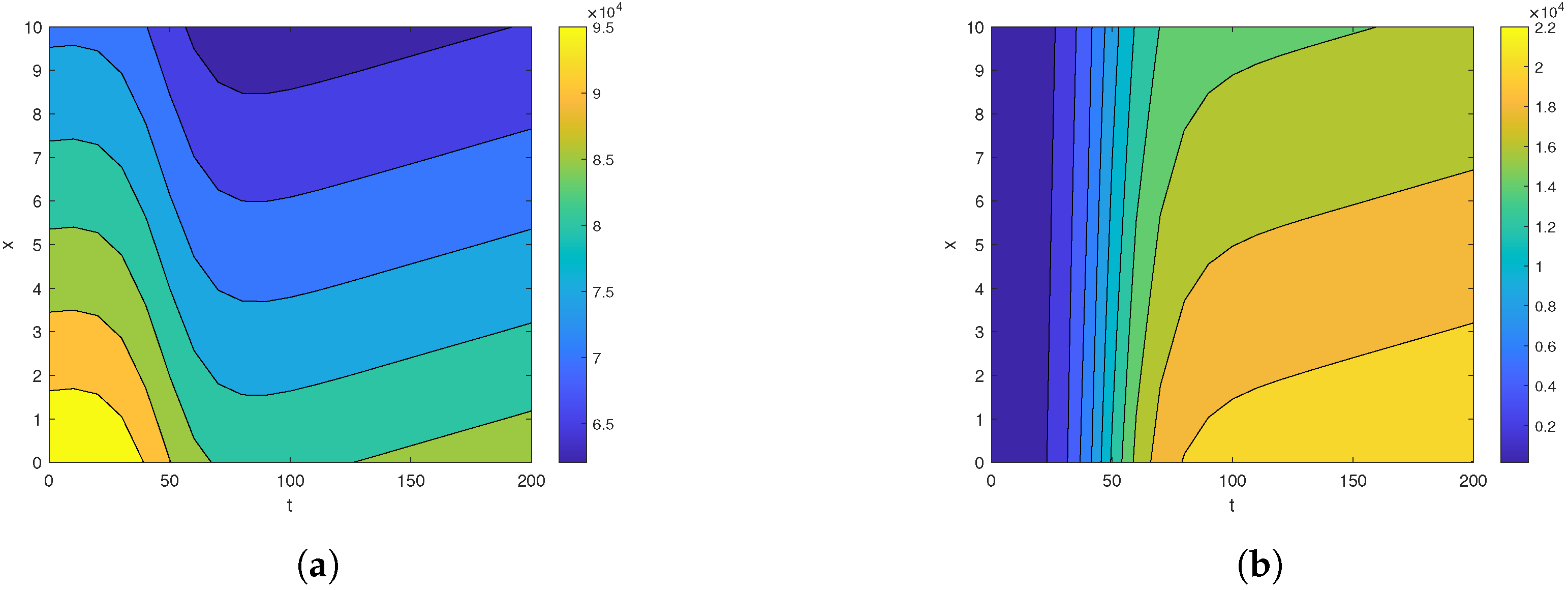
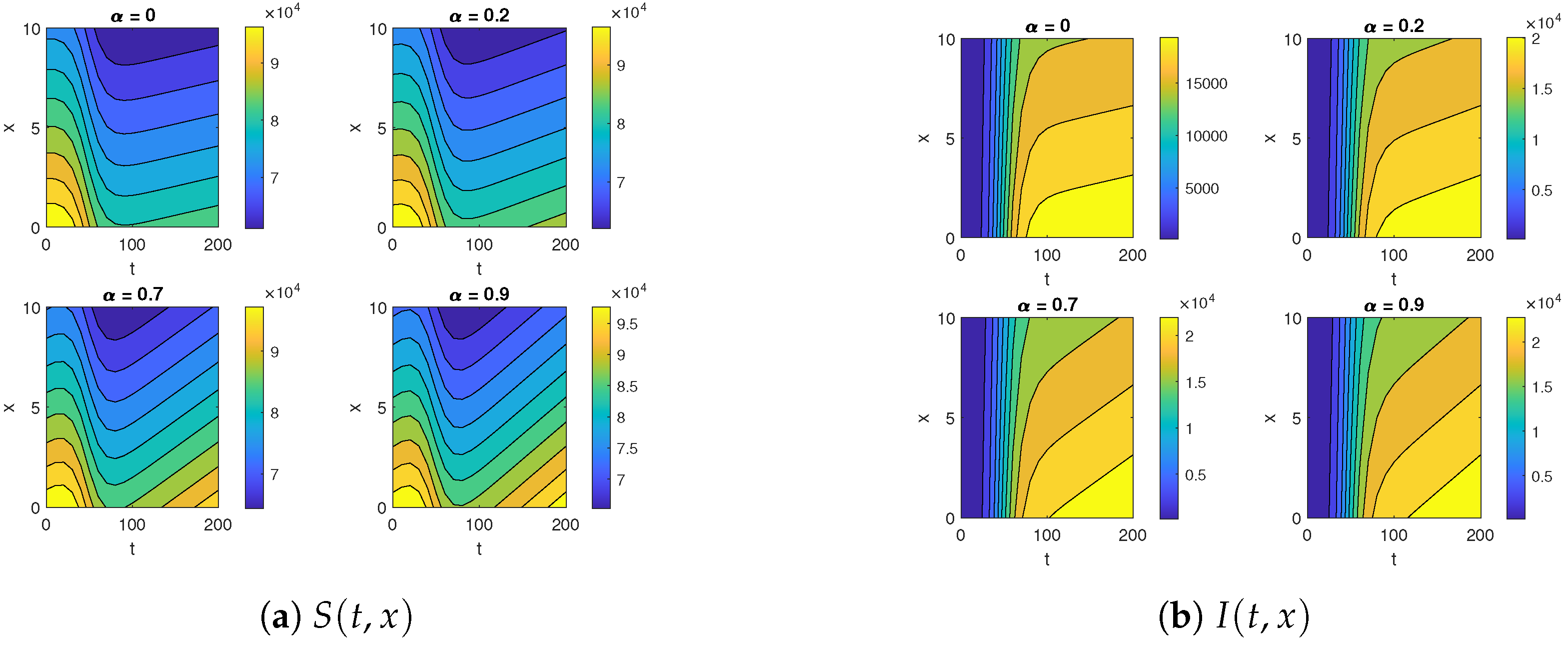
Figure 2. The contour map for (a) $S(t,x)$ and (b) $I(t,x)$ for $S_0={10}^5-200$, $I_0=200$, $\lambda =0.03$, $\alpha =0.2$, $\beta =0.5$, $\gamma =0.4$, and $\theta =0.01$ over the time intervals $0\le t\le 200$ and $0\le x\le 10$.

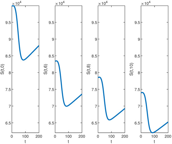
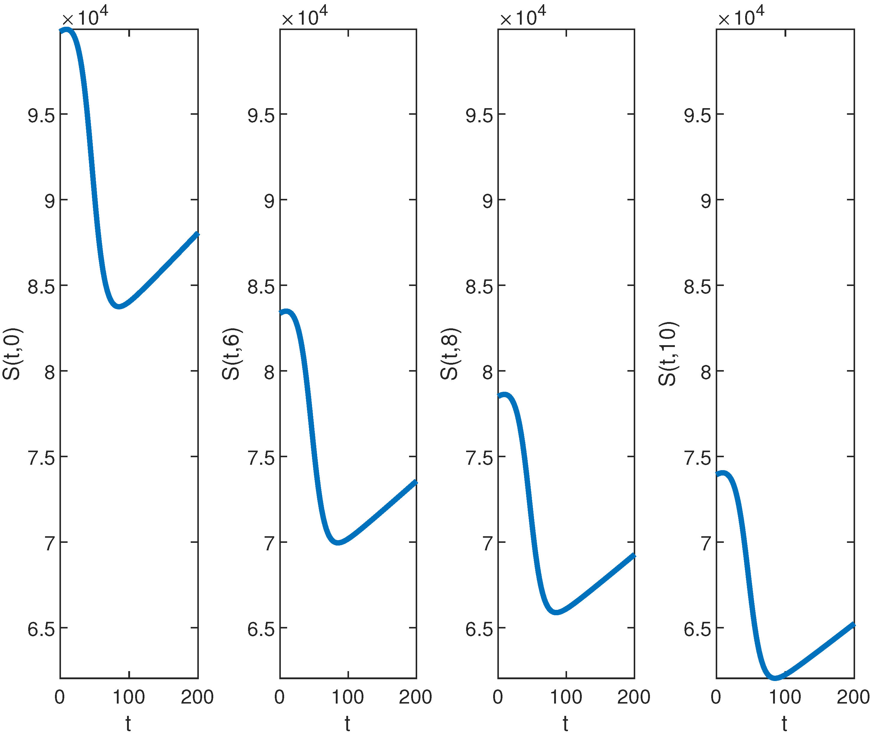
Figure 3. The graph of $S(t,\overline{x})$ for $S_0={10}^5-200$, $I_0=200$, $\lambda =0.03$, $\alpha =0.2$, $\beta =0.5$, $\gamma =0.4$, and $\theta =0.01$ over the time interval $0\le t\le 200$ and for fixed values of $x=0,6,8,10$.

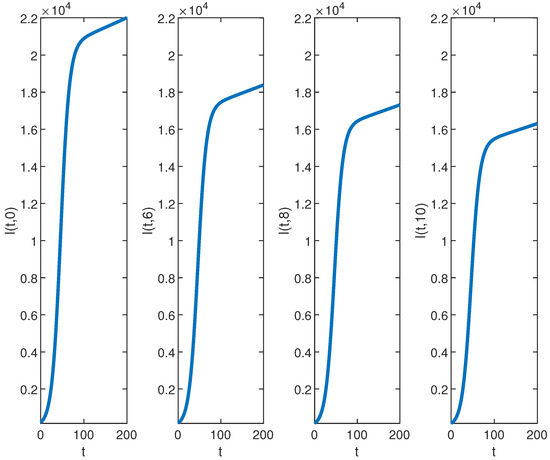
Figure 4. The graph of $I(t,\overline{x})$ for $S_0={10}^5-200$, $I_0=200$, $\lambda =0.03$, $\alpha =0.2$, $\beta =0.5$, $\gamma =0.4$, and $\theta =0.01$ over the time interval $0\le t\le 200$ and fixed values of $x=0,6,8,10$.

First, we analyze the behavior of the susceptible population $S(t,x)$ from Figure 1a, Figure 2a, and Figure 3. At the disease source, located at $x=0$, the susceptible population initially decreases before showing an upward trend after a certain period, indicating a long-term increase. This same pattern is observed at other locations such as $x=6,8,10$. The number of susceptible individuals is highest at $x=0$ and decreases as we move away from the disease source. Specifically, the graphs show the highest susceptibility at $x=0$ and the lowest at $x=10$.

Our analysis now shifts to the density of the infected population $I(t,x)$ highlighted in Figure 1b, Figure 2b, and Figure 4. At the disease source located at $x=0$, the number of infected individuals initially increases before taking a sudden turn after a certain period, continuing to increase steadily thereafter. A similar pattern is observed at other locations such as $x=6,8,10$. The highest number of infected individuals is observed at $x=0$, and the count decreases as we move away from the disease source. Specifically, the graphs show the highest number of infections at $x=0$ and the lowest at location $x=10$.

4.3. Effect of Varying the Diffusion Coefficient on Susceptible and Infected Populations

Figure 5 and Figure 6 illustrate the impact of varying the diffusion coefficient, denoted as $\alpha$, on both susceptible and infected populations. The increase in the diffusion coefficient leads to a higher influx of individuals into the susceptible compartment, reflecting an increased movement of people into the location from external sources. Shifting our focus to the infected compartment, it is evident that the infected population also rises with the increase in the diffusion coefficient. This makes sense, as the movement of infected individuals contributes to the transmission of the infection to previously healthy individuals.

Figure 5. The contour maps for (a) $S(t,x)$ and (b) $I(t,x)$ for different diffusion coefficients $\alpha$.

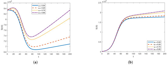
Figure 6. The graph of (a) $S(t,6)$ and (b) $I(t,6)$ for different diffusion coefficients $\alpha$.

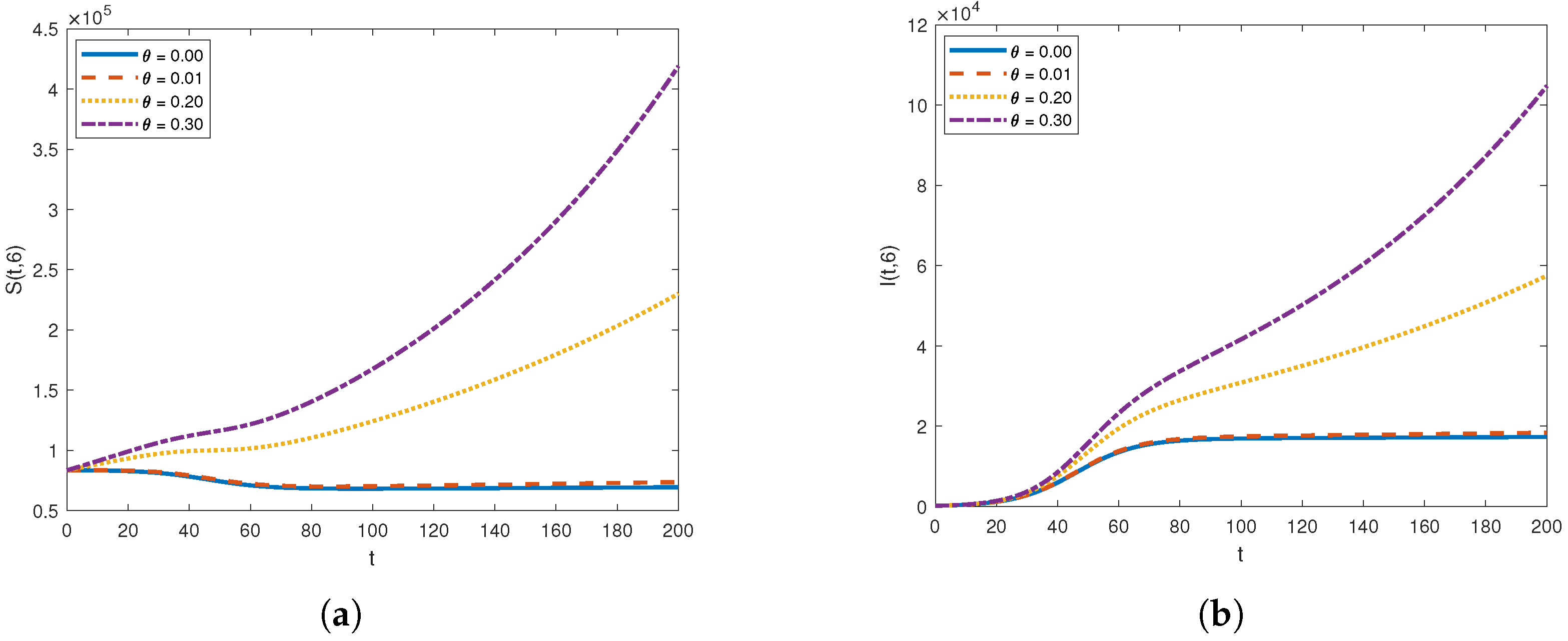
4.4. Effect of Varying the Advection Rate on Susceptible and Infected Populations

Figure 7 and Figure 8 illustrate the impact of varying the advection rate, denoted as $\theta$, on both susceptible and infected populations. For smaller values of the advection rate, such as $\theta =0$ and $\theta =0.01$, the susceptible population initially decreases and then stabilizes. Shifting our focus to the infected compartment, for these same smaller advection rates, the infected population initially increases and then stabilizes. This pattern is logical as individuals leave the susceptible compartment and enter the infected compartment. Over time, due to better disease management and precautionary measures, both the susceptible and infected populations stabilize.

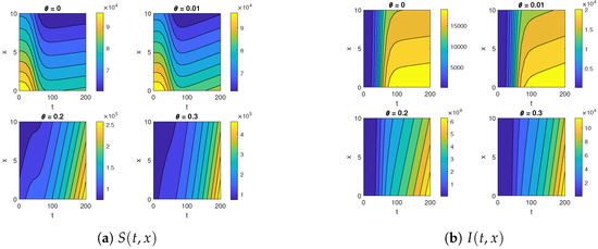
Figure 7. The contour maps for (a) $S(t,x)$ and (b) $I(t,x)$ for a different advection velocity $\theta$.

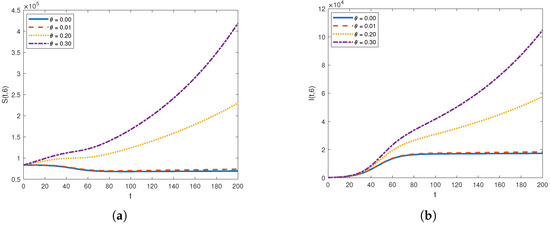
Figure 8. The graph of (a) $S(t,6)$ and (b) $I(t,6)$ for a different advection velocity $\theta$.

Shifting our focus to the higher values of the advection rate, both the susceptible and infected populations increase. This significant rise in the advection rate results in a greater influx of individuals into the susceptible compartment, reflecting the heightened movement of people into the location from external sources. It is clear that the infected population also rises with the increase in the advection rate. This is expected, as the movement of infected individuals facilitates the transmission of the infection to previously healthy individuals.

5. Conclusions

This work explored a class of SIS epidemic model with reaction–diffusion–advection by utilizing the Lie group methods. Lie symmetries were established for three widely utilized incidence functions: standard, mass action, and saturated. The SIS-RDA model exhibited a four-dimensional Lie algebra with the standard incidence function, a three-dimensional Lie algebra with mass action incidence, and a two-dimensional Lie algebra with saturated incidence.

The investigation of the SIS-RDA epidemic model for the standard incidence infection mechanism was extended. We explored several reductions and closed-form solutions by employing linear combinations of Lie symmetries. The transmission dynamics of an infectious disease utilizing closed-form solutions were presented. The solution to the Cauchy problem provided insights into the trajectories of susceptible and infected populations. We showed how the paths of susceptible and infected populations develop over time with parameter values sourced from the existing literature. Furthermore, a sensitivity analysis was conducted to provide insights into potential policy recommendations for the control of the disease.

It is worth mentioning here that we have tested the closed-form solution for a set of parameter values taken from the literature. Parameter values from the data of any specific country can be employed to analyze the derived closed-form solution and understand the transmission dynamics of the infectious disease.

References

- Allen, L.J.S.; Bolker, B.M.; Lou, Y.; Nevai, A.L. Asymptotic profiles of the steady states for an SIS epidemic reaction-diffusion model. Discret. Contin. Dyn. Syst. 2008, 21, 1–20. [Google Scholar] [CrossRef]
- Fitzgibbon, W.E.; Langlais, M.; Morgan, J.J. A mathematical model of the spread of feline leukemia virus (FeLV) through a highly heterogeneous spatial domain. SIAM J. Math. Anal. 2001, 33, 570–588. [Google Scholar] [CrossRef]
- Fitzgibbon, W.E.; Langlais, M.; Morgan, J.J. A reaction-diffusion system modeling direct and indirect transmission of diseases. Discrete Contin. Dyn. Syst. Ser. B 2004, 4, 893–910. [Google Scholar] [CrossRef]
- Peng, R.; Liu, S. Global stability of the steady states of an SIS epidemic reaction-diffusion model. Nonlinear Anal. Theory Methods Appl. 2009, 71, 239–247. [Google Scholar] [CrossRef]
- Veliov, V.M. On the effect of population heterogeneity on dynamics of epidemic diseases. J. Math. Biol. 2005, 51, 123–143. [Google Scholar] [CrossRef]
- Gudelj, I.; White, K.A.J.; Britton, N.F. The effects of spatial movement and group interactions on disease dynamics of social animals. Bull. Math. Biol. 2004, 66, 91–108. [Google Scholar] [CrossRef] [PubMed]
- Lutscher, F.; Lewis, M.A.; McCauley, E. Effects of heterogeneity on spread and persistence in rivers. Bull. Math. Biol. 2006, 68, 2129–2160. [Google Scholar] [CrossRef]
- Desai, M.M.; Nelson, D.R. A quasispecies on a moving oasis. Theor. Popul. Biol. 2005, 67, 33–45. [Google Scholar] [CrossRef]
- Cui, R.; Lou, Y. A spatial SIS model in advective heterogeneous environments. J. Differ. Equ. 2016, 261, 3305–3343. [Google Scholar] [CrossRef]
- Jiang, D.; Wang, Z.C.; Zhang, L. A reaction-diffusion-advection SIS epidemic model in a spatially-temporally heterogeneous environment. Discret. Contin. Dyn. Syst. Ser. B 2018, 23, 4557–4578. [Google Scholar] [CrossRef]
- Cui, R.; Li, H.; Peng, R.; Zhou, M. Concentration behavior of endemic equilibrium for a reaction-diffusion-advection SIS epidemic model with mass action infection mechanism. Calc. Var. Partial. Differ. Equ. 2021, 60, 184. [Google Scholar] [CrossRef]
- Zhang, J.; Cui, R. Asymptotic behavior of an SIS model with saturation and spontaneous infection mechanism. Z. Angew. Math. Phys. 2020, 71, 1–21. [Google Scholar] [CrossRef]
- Ge, J.; Kim, K.I.; Lin, Z.; Zhu, H. A SIS-advection model in a low-risk and high-risk domain. J. Differ. Equ. 2015, 259, 5486–5509. [Google Scholar] [CrossRef]
- Rao, X.; Zhang, G.; Wang, X. A reaction-diffusion-advection SIS epidemic model with linear external source and open advective environments. Discret. Contin. Dyn. Syst. Ser. B 2022, 27, 6655–6677. [Google Scholar] [CrossRef]
- Bluman, G.W.; Cole, J.D. Similarity Methods for Differential Equations; Springer: New York, NY, USA, 1974. [Google Scholar]
- Ovsiannikov, L.V. Group Analysis of Differential Equations; Academic Press: New York, NY, USA, 1982. [Google Scholar]
- Ibragimov, N.H. Transformation Groups Applied to Mathematical Physics; Reidel: Dordrecht, The Netherlands, 1985. [Google Scholar]
- Olver, P.J. Applications of Lie Groups to Differential Equations; Springer: New York, NY, USA, 1986. [Google Scholar]
- Bluman, G.W.; Kumei, S. Symmetries and Differential Equations; Springer: Berlin, Germany, 1989. [Google Scholar]
- Ibragimov, N.H. CRC Handbook of Lie Group Analysis of Differential Equations; CRC Press: Boca Raton, FL, USA, 1996. [Google Scholar]
- Cantwell, B.J. Introduction to Symmetry Analysis; Cambridge University Press: Cambridge, UK, 2002. [Google Scholar]
- Ibragimov, N.H. A Practical Course in Differential Equations and Mathematical Modelling; World Scientific Publishing Co Pvt Ltd.: Singapore, 2009. [Google Scholar]
- Senthilvelan, M.; Torrisi, M. Potential symmetries and new solutions of a simplified model for reacting mixtures. J. Phys. A Math. Gen. 2000, 33, 405. [Google Scholar] [CrossRef]
- Torrisi, M.; Tracinà, R. An application of equivalence transformations to reaction diffusion equations. Symmetry 2015, 7, 1929–1944. [Google Scholar] [CrossRef]
- Wang, G. A new (3 + 1)-dimensional Schrödinger equation: Derivation, soliton solutions and conservation laws. Nonlinear Dyn. 2021, 104, 1595–1602. [Google Scholar] [CrossRef]
- Cherniha, R.M.; Davydovych, V.V. A reaction-diffusion system with cross-diffusion: Lie symmetry, exact solutions and their applications in the pandemic modelling. Eur. J. Appl. Math. 2022, 33, 785–802. [Google Scholar] [CrossRef]
- Freire, I.L.; Da Silva, P.L.; Torrisi, M. Lie and Noether symmetries for a class of fourth-order Emden-Fowler equations. J. Phys. A Math. Theor. 2013, 46, 245206. [Google Scholar] [CrossRef]
- Naz, R.; Johnpillai, A.; Mahomed, F.M.; Omame, A. Closed-form solutions for a reaction-diffusion SIR model with different diffusion coefficients. Discret. Contin. Dyn. Syst. Ser. S 2024. [Google Scholar] [CrossRef]
- Naz, R.; Johnpillai, A.; Mahomed, F.M. The exact solutions of a diffusive SIR model via symmetry groups. J. Math. 2024, 2024, 4598831. [Google Scholar] [CrossRef]
- Cheviakov, A.F.; Zhao, P. Analytical Properties of Nonlinear Partial Differential Equations: With Applications to Shallow Water Models; Springer Nature: Berlin/Heidelberg, Germany, 2024; Volume 10. [Google Scholar]
- Hereman, W. Symbolic software for Lie symmetry analysis. In CRC Handbook of Lie Group Analysis of Differential; CRC: Boca Raton, FL, USA, 1996; Volume 3, pp. 367–413. [Google Scholar]
- Hereman, W. Review of symbolic software for Lie symmetry analysis. Math. Comput. Model. 1997, 25, 115–132. [Google Scholar] [CrossRef]
- Cheviakov, A.F. GeM software package for computation of symmetries and conservation laws of differential equations. Comput. Phys. Commun. 2007, 176, 48–61. [Google Scholar] [CrossRef]
- Takahashi, L.T.; Maidana, N.A.; Ferreira, W.C.; Pulino, P.; Yang, H.M. Mathematical models for the Aedes aegypti dispersal dynamics: Travelling waves by wing and wind. Bull. Math. Biol. 2005, 67, 509–528. [Google Scholar] [CrossRef]
- Bacani, F.; Dimas, S.; Freire, I.L.; Maidana, N.A.; Torrisi, M. Mathematical modelling for the transmission of dengue: Symmetry and travelling wave analysis. Nonlinear Anal. Real World Appl. 2018, 41, 269–287. [Google Scholar] [CrossRef]
Disclaimer/Publisher’s Note: The statements, opinions and data contained in all publications are solely those of the individual author(s) and contributor(s) and not of MDPI and/or the editor(s). MDPI and/or the editor(s) disclaim responsibility for any injury to people or property resulting from any ideas, methods, instructions or products referred to in the content. |
© 2024 by the authors. Licensee MDPI, Basel, Switzerland. This article is an open access article distributed under the terms and conditions of the Creative Commons Attribution (CC BY) license (https://creativecommons.org/licenses/by/4.0/).