Abstract
Natural and unconstrained locomotion remains a fundamental challenge in creating truly immersive virtual reality (VR) experiences. This paper presents the design and control of a novel robotic omnidirectional treadmill (ODT) based on the bilateral symmetry of two cooperative five-bar planar mechanisms designed to replicate realistic walking mechanics. The central contribution is a human in the loop control strategy designed to achieve stable walking in place. This framework employs a specific control strategy that actively repositions the footplates along a dynamically defined ‘Line of Movement’ (LoM), compensating for the user’s motion to ensure the midpoint between the feet remains stabilized and symmetrical at the platform’s geometric center. A comprehensive dynamic model of both the ODT and a coupled humanoid robot was developed to validate the system. Numerical simulations demonstrate robust performance across various gaits, including turning and catwalks, maintaining the user’s locomotion center with a maximum resultant drift error of 11.65 cm, a peak value that occurred momentarily during a turning motion and remained well within the ODT’s safe operational boundaries, with peak errors along any single axis remaining below 9 cm. The system operated with notable efficiency, requiring RMS torques below 22 Nm for the primary actuators. This work establishes a viable dynamic and control architecture for foot-tracking ODTs, paving the way for future enhancements such as haptic terrain feedback and elevation simulation.
1. Introduction
ODTs are defined as platforms that enable users to experience 360-degree motion within a virtual reality environment, without changing their position in the physical world. The lack of realistic interaction between real and VR environments represents a significant obstacle to the integration of these two systems. To address this challenge, this paper introduces a novel robotic ODT system operating under a human in the loop (HIL) control paradigm. Unlike passive or preprogrammed systems, robotic ODT dynamically adapts to the user’s real-time movements, tracking foot trajectories and intended direction to create a responsive and boundless walking experience. This work introduces a novel concept called the ‘Line of Movement’ (LoM), where a control strategy actively guides the footplates to keep the user’s stance centered on the platform. Conceptually, the user stands on two independent footplates, each manipulated by a five-bar mechanism. The system uses external sensors (such as IMUs or a motion capture system) to track the real-time position of the user’s feet. This position data serves as a command signal for the robotic platform, which actively moves the footplates to follow the user’s natural gait cycle. By precisely repositioning the ground beneath the user’s feet, the ODT allows for walking, turning, and other movements while keeping the user safely at the center of the platform. Future iterations of robotic ODT promise to enhance VR experiences further by integrating haptic feedback and elevation capabilities, allowing users to interact with diverse virtual terrains. This solution holds the potential to enable activities such as stair climbing, navigating uneven surfaces, and simulating walking in challenging environments like mud, snow, and ice. For illustrative purposes, an animation is provided in Figure 1.
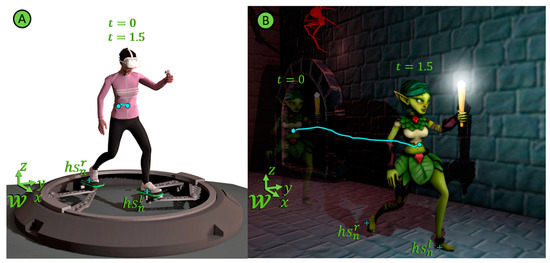
Figure 1.
Demonstration and animation of the robotic ODT in the physical world (A) and virtual reality environment (B). (https://www.youtube.com/watch?v=xZVAJOYcB8E, Accessed: [14 June 2025]).
A comprehensive list of current VR locomotion techniques can be found in this study [1]. While numerous applications exist for VR locomotion, the latest and most advanced studies in the literature are presented below. Current ODTs can be broadly categorized by their mechanical approach, each with distinct limitations. The most common are slip-style treadmills, which use surfaces like low-friction bowls (e.g., Virtuix Omni) or actuated rollers/belts to allow the user’s feet to slide back to the center [2,3,4]. Figure 2 depicts the VR slip-style treadmill, which is currently the only model available as a commercial product. While commercially available, these systems do not replicate natural walking mechanics. Studies have shown that the non-natural gait required on such platforms can negatively impact user experience, task performance, and even induce higher levels of cybersickness compared to more conventional locomotion [5,6]. Hooks et al. showed that the bowl-based omnidirectional treadmill outperformed the flat-based one in ergonomics and user control, with a clear preference from participants. It performed better over short distances, while no significant differences were found for long distances [7]. Another approach involves ball- or sphere-based systems, where a user walks on a large, rotating sphere. These designs often suffer from high mechanical complexity, significant inertia, and challenges in providing consistent and reliable motion control.
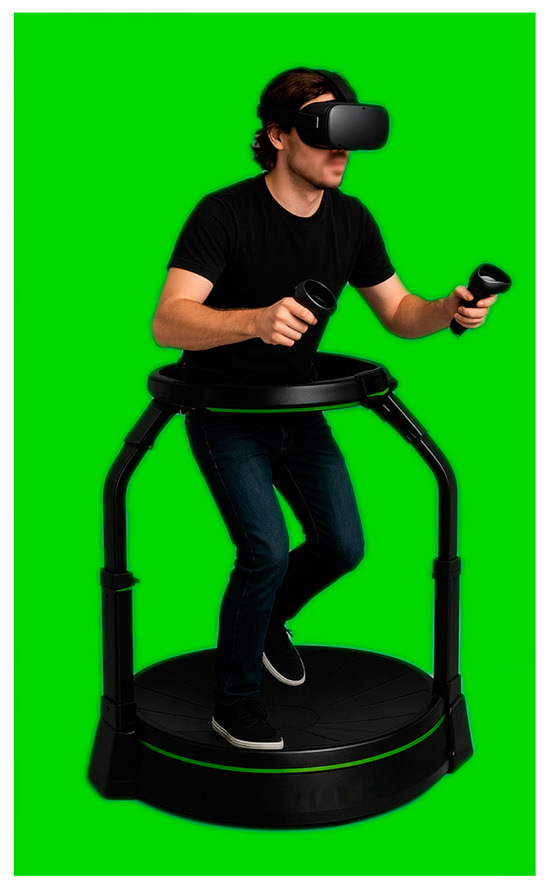
Figure 2.
The images depict slip-style treadmills, which are currently the only commercially available models. These systems allow users to move in virtual environments by sliding their feet over low-friction surfaces, but they do not fully replicate the mechanics of natural walking.
Otaran and Farkhatdinov introduced an impedance-based ankle haptic interface for immersive navigation in VR, allowing users to experience natural walking through foot-tapping gestures while seated. The system effectively rendered different terrain types, including hard, soft, and complex multi-layered surfaces. However, limitations include the use of a single DoF platform, which may not fully capture the dynamics of natural leg movements, and challenges in simulating precise walking kinematics [8]. Kim et al. introduced a walking-in-place technique for omnidirectional VR using a single RGB camera and OpenPose, achieving a stable virtual walking speed compared to Kinect-based methods, especially in non-frontal directions. However, the method falls short of providing a true sense of real walking, affecting the overall immersion in the VR experience [9]. Choi et al. introduce the Seamless-walk system, a VR locomotion approach that leverages high-resolution tactile sensors to enable natural walking without wearable devices. The system translates foot pressure data into movement signals using machine learning, offering advantages over traditional methods in terms of comfort and privacy. However, jumping and continuous walking are not well integrated [10].
The results demonstrate that VR locomotion provides significant advantages for physical therapy. Numerous studies in the literature have demonstrated that treadmill designs enabling natural walking motion can be highly beneficial.
Zenner et al. proposed Saccadic and Blink-Suppressed Hand Redirection (SBHR), which combines saccadic and blink-induced change blindness for improved hand redirection in VR. Unlike previous techniques that relied only on blinks, SBHR integrates gradual drifting with shifts during saccades and blinks, enabling more frequent redirection. While this approach addresses the limitations of blink-based methods, its effectiveness depends on parameter tuning and quality of eye tracking [11]. Sun et al. introduced a novel approach called Dynamic Saccadic Redirection to address the challenge of infinite walking in VR by leveraging saccadic suppression to imperceptibly redirect users during rapid eye movements. Their system utilizes real-time path planning and subtle gaze direction to dynamically avoid static and moving obstacles, allowing users to explore large virtual environments within smaller physical spaces. However, the method may not fully account for complex, dynamic multi-user scenarios [12].
Hwang et al. introduced the REVES system, a novel approach to enhancing redirected walking using four-pole galvanic vestibular stimulation. Using galvanic vestibular stimulation, the REVES system extended the range for detecting redirected walking, particularly in rotation and walking direction adjustments [13]. Groth et al. present omnidirectional GVS to reduce cybersickness in VR by aligning electrical stimulation with visual motion, significantly improving user comfort [14]. Smith et al. introduce a wearable device using GVS to enhance virtual reality experiences by reducing cybersickness and increasing immersion. While the device shows promising results in a user study, the limited sample size and short-term evaluation present areas for further research [15]. Joint servos constitute 60% of the robot’s design cost, highlighting the actuation system as a key area for future optimization. Recent advancements in tribology and mechanical component design offer promising methods for enhancing the durability and efficiency of such systems [16,17].
Symmetry is a fundamental concept in both robotics and human biomechanics. In robotics, exploiting structural symmetries simplifies system modeling and leads to more efficient and robust control algorithms. In human locomotion, walking is an inherently periodic and largely symmetric motion, where the movement of one leg mirrors the other with a phase shift. Consequently, the fundamental requirement for an immersive VR treadmill comprises two interrelated aspects: the mechatronic system must exhibit a bilaterally symmetric architecture to be kinematically compatible with human bipedal locomotion, and its control framework must be capable of dynamically regulating this symmetry to ensure the user remains stabilized at the platform’s operational center. This study addresses this challenge by introducing a robotic ODT with a bilaterally symmetric mechanical design and a control strategy that explicitly leverages the principles of symmetry to ensure stable and natural walking in place.
The following assumptions were taken into account in the design of the robotic ODT:
- This study assumes that control is conducted based on the free-body diagram; additionally, the links of the five-bar robotic mechanism can be positioned in various configurations to ensure that they do not intersect with each other [18]. For example, the bases can move along separate circular paths to prevent collisions. Link configuration is provided in the Appendix A.
- A no-slip condition is assumed at the contact interface. In the simulation, where the humanoid foot is modeled with a point contact, this condition is enforced by applying a sufficiently high coefficient of friction to prevent tangential sliding under the calculated ground reaction forces. This is a practical idealization, as the physical footplate is envisioned to be coated with a high-friction, rubber-like material, which would make slip a rare event during normal walking gaits.
- It is assumed that the robotic ODT has real-time information on the foot tip positions of the humanoid model. In practical applications, this data can be obtained through inertial measurement unit (IMU) or motion capture (MOCAP) techniques [19].
For more accessible or prototype applications, it is also feasible to determine foot position using simpler, vision-based methods, such as basic color tracking or marker detection with a standard RGB camera. This demonstrates the adaptability of the control architecture to different hardware levels.
- The creation of a realistic human model for the purpose of testing the robotic ODT represents a significant challenge; a reduced model designed to meet dynamic stability criteria was created.
- All limbs in the simulation are assumed to be rigid.
This paper is structured as follows. Section 2 details the kinematic and dynamic modeling of both the dual five-bar ODT and the coupled humanoid robot, establishing the mathematical foundation for the control design. Section 3 introduces the core contribution: the walking-in-place control strategy designed to maintain user stability. Section 4 provides numerical simulations to validate the proposed method, where graphical results are analyzed to demonstrate performance. Finally, Section 5 concludes the paper by summarizing the key findings and providing recommendations for future work.
2. Kinematic and Dynamic Modeling
2.1. Robotic ODT
The ODT’s design is founded on the principle of bilateral symmetry, utilizing two identical five-bar mechanisms, one for each foot. This symmetric architecture is crucial for naturally replicating bipedal locomotion. In our system, the typically fixed link 5 is configured to move freely along the perimeter of a constrained circular path. Figure 3 illustrates the top view and definitions of the planar walking platform. In each robotic mechanism, the base link 5 is driven by an actuator to enable movement along the periphery of a circular path. Thus, the robotic mechanisms are enabled to rotate around the circular path, and position control is achieved through the torques , where . The world frame is defined as . The center point of the circular path is designated as . The distance from the center of the circular path to the axis is represented by . The angle of this line is represented by . The angle of the robotic mechanism’s base link 5 or axis is given by parameter . The design-based relationship between and is provided in Equation (2). The location of the end effector is indicated by . In each robotic mechanism, links 1 and 4 are actuated by and to allow continuous tracking of the foot positions. Links 2 and 3 remain passive. Safe regions have been defined for the footplates to achieve a singularity-free workspace. represents the workspace defined for the end point , while denotes the safe boundaries of the footplate. The workspaces of both mechanisms can move freely within , the operational area of the ODT. An additional degree of freedom has been added at the end effector point, where link 6, the footplate supporting the foot, is connected to a joint at this location. The orientation control of the plates is achieved through the torque . In the robotic five-bar mechanism, the link lengths , link weights , and inertias are defined for .
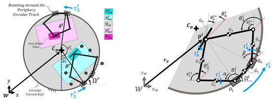
Figure 3.
Free-body diagram of proposed robotic ODT platform (left); kinematic and dynamic representations for the footplate (right).
In the dynamic analysis of articulated systems, the equation of motion commonly employed for both legged robots and general mechanisms can be expressed using either the Newton–Euler or Lagrange methods in Equation (1):
In this equation, denotes the generalized coordinate vector representing joint angles in a legged robot or degrees of freedom in a mechanism, while and represent the vectors of generalized velocities and accelerations, respectively. Each term in the equation is defined as follows:
: The mass or inertia matrix, representing the mass distribution and inertia properties of the system.
: The Coriolis and centrifugal forces term, taking complex effects on system dynamics.
: The gravitational force term.
: The vector of external torques or forces acting on the joints or degrees of freedom, representing the active actuation forces applied to the system.
: The Jacobian matrix of the system.
: The external force vector acting on the end effector; in legged robots, ground reaction forces.
This general formulation encompasses the dynamics of multi-joint motions in both legged robots and mechanisms. Therefore, it enables the modeling of the necessary forces and torques required to achieve the desired motion in these systems. Both the ODT and the humanoid robot’s dynamic models were developed using MATLAB 2024b Simulink to produce the same results as the equations of motion, providing a comprehensive framework for simulating and analyzing motion and control behavior. A structural viscous damping amount of 0.005 defined for all joints to represent inherent frictional losses and to enhance numerical stability. The simulation employed a fixed-step, fourth-order ode4 (Runge–Kutta) solver with a time step of This combination was chosen as it represents a well-established and efficient method for continuous multi-body dynamics. The step size was selected to balance numerical accuracy with computational efficiency; smaller steps yielded negligible changes in results, while larger steps caused instability. The complete system architecture of the robotic ODT’s dynamics and control structures, developed in MATLAB Simulink, is provided in the Appendix A.
The forward kinematics of the ODT were determined using the equations provided below. The rotation matrix relative to point is defined by the angle . This angle is related to the position angle of the mechanism’s base, , by a constant design offset α_offset, as established in Equation (2). This offset is a direct geometric consequence of the mechanical design, specifically chosen to ensure that both pivots of the base link (Link 5), and , remain perfectly constrained on the circular guide rail. Given the fixed diameter of the rail and the length of Link 5, this constant angular displacement (α_offset = 0.0405295 * π rad) is mathematically necessary to satisfy the kinematic constraint.
The distance of from the inertial frame, denoted as , is provided in Equation (3). The expanded form of this equation is presented in Equation (4).
The Jacobian calculation for the five-bar robot, which differs from standard robotic arms due to its closed-chain structure, is outlined below. Starting from point , the system is divided into two separate robotic arms, and the Jacobians for each side are determined. Formulation can be found in [20]. In the robotic mechanism, represents the Jacobian for links 1 and 2, while represents the Jacobian for links 3 and 4, as specified in Equation (5). Terms and are provided in Equation (6).
Given that , ,
By excluding the non-actuated joints in this setup,
. The velocity of the end effector relative to the axis is given in Equation (7).
The linear velocity of point relative to the inertial frame is given in Equation (8).
The inverse kinematics of the ODT are calculated using the set of equations provided below. The x and y distances between and are computed in Equation (9). The terms and represent the desired reference x and y positions of the footplate.
From here, the angles and are calculated using the formulas provided in Equations (10) and (11).
where
where
2.2. Humanoid Robot with Point Contact
In order to test the developed dynamic platform model, it is necessary to have contact forces that can interact with the footplate, as well as a dynamic human model capable of walking. The front of the robot model is aligned with the x-axis. The floating axis on the robot’s body is positioned at the geometric center of the rectangular prism, which also corresponds to the center of mass. The position of the base axis relative to the fixed world axis is represented by . Each leg of the robot is connected through rotational joints, providing four degrees of freedom (DOFs) per leg. The leg and body dimensions are denoted by . To derive the kinematic expressions, coordinate axes are assigned to the joints, as illustrated in Figure 4. A Simulink diagram illustrating the dynamics of the humanoid robot is provided in the Appendix A. The two limb segments of the leg have equal mass and inertia values.
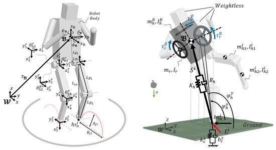
Figure 4.
Kinematic illustrations (left) and dynamic illustrations for the humanoid model (right).
The Denavit–Hartenberg parameters provide the most general form of the homogeneous transformation matrix between link and link , as shown in Equation (12). In this equation, denotes the rotation matrix, and represents the position vector. The established D-H parameters are presented in Table 1.

Table 1.
D-H parameters for the first and second leg.
The transformation matrix for the robot’s foot tip relative to the first axis set is obtained by multiplying the following four homogeneous transformation matrices, as shown in Equation (13).
The forward kinematic expressions for the robot’s foot tip positions relative to the axis set are provided in Equation (14).
The transformation of the base frame with respect to the fixed ground frame is given by Expression (15).
Based on this, the coordinates of each foot of the humanoid model, , relative to the ground frame, are calculated using Expression (16). Here, and represent the distances between the femur and the foot tip.
In analyzing the locomotion of the humanoid model, certain trajectories for the foot are predefined. For the robot to follow these paths, its legs must reach the specified coordinates during movement. As a result, the joint angles of the legs need to be computed using inverse kinematics to align with these target coordinates. The kinematic diagram of a leg, as illustrated in Figure 4, was used for the inverse kinematic analysis of each leg. The aim is to determine the joint angles for that align the leg with the specified reference foot tip coordinates. The geometric method for solving the inverse kinematics of the humanoid leg is provided below. The angles and for joints 1 and 2 can be readily determined by substituting the foot coordinates (, , ) into Expression (17).
In the kinematic model depicted in Figure 4, is computed using Expression (18) by applying a series of equations. Subsequently, is also obtained through Expression (18).
The humanoid robot’s walking motion is examined in two separate phases: the ground phase and the flight phase.
2.2.1. Humanoid Leg Tip on Ground Stage
Since obtaining a realistic dynamic human model is very challenging, we simplified our model and applied Cartesian impedance control, a well-known method in legged robots. Additionally, the orientation of the underactuated robot body was controlled using reaction wheels, with torsional impedance control applied. In certain studies on legged robots, dynamic models utilizing reaction wheels have been developed to achieve the target orientations of the underactuated main body, supporting balanced and stable walking [21]. Lee et al. successfully enhanced the balance of a quadruped robot using a reaction wheel, enabling the robot to walk along a straight line [22]. The robot’s foot tips are modeled as point contacts, and torques are applied to the joint actuators in the legs as a result of impedance control, with stabilization achieved through the reaction wheel. The velocity information required for Cartesian impedance control was determined. The x, y, and z components of the velocity change between the foot tip of the contacting leg and the body center are provided in Equations (19)–(21).
where
where
where
During the ground stage, the torque matrix applied to the body and the leg in contact with the ground is represented as in Equation (22). Here, represents the torques applied to the reaction wheel along the body axis, while denotes the control torques applied to the leg joints. The control gains and are the torsional impedance control coefficients that maintain body orientation. and are the torsional impedance control coefficients that regulate the angle . The Cartesian impedance control coefficients for the body center relative to the foot tip, as shown in Figure 4, are denoted by and . The resulting forces are mapped to the joints, yielding the torques and . The control torque is multiplied by the coefficient to stabilize the reaction wheels that control the base rotations against changes in the direction of .
where
2.2.2. Humanoid Leg Tip in Flight Stage
While the body is balanced and supported on one leg, the foot tip of the other leg follows a predefined trajectory. During trajectory tracking, reference angles for the leg joints are determined using inverse kinematics and tracked with a PD controller. In the flight phase, the legs follow a sinusoidal trajectory function along the z-axis to facilitate stepping. Each leg transitions to the ground phase after a total duration of one second. In the functions provided in Equation (23), and represent the step length in the z and x axes, respectively, and denotes the fixed time step of the simulation.
As a result of the inverse kinematics, the desired angular trajectories are obtained. The error is defined as . In the designed controller, the proportional and derivative gains, and , were optimized using a trial-and-error method. Consequently, the control torques are applied to the specified joints in the humanoid leg. The contact surface between the tip of the humanoid leg and the ground is assumed to be a point. The vertical and horizontal contact forces at point are presented in Equation (24).
The contact forces at point are represented by . As illustrated in the dynamic model in Figure 4, the ground interaction mechanics are modeled in the vertical direction using a linear spring–damper system. The ground stiffness is represented by and the viscous damping coefficient by . These parameters, which were empirically tuned using simulated drop tests to achieve a realistic contact response, are explicitly listed as and in the Humanoid Robot Parameters section of the table. When point contacts the ground, it is assumed that there is no slip, and the first derivative of the foot tip point satisfies .
3. ODT Walking-in-Place Control: A Human in the Loop Approach
The control of the robotic ODT is a human in the loop problem, and the core of our control strategy is to maintain a dynamic symmetric equilibrium. The system’s primary goal is not to follow a predefined trajectory, but to react to the unpredictable movements of the human user to keep them safely centered on the platform. To achieve stable and natural walking in place, we developed a control framework, the architecture of which is presented below. This framework is designed to manage the complex interactions between the user’s movements and the ODT’s response by systematically deploying a set of state-dependent control modules. The core of our control strategy is to maintain a dynamic symmetric equilibrium.
3.1. ODT Control During Humanoid Leg in Flight Stage
When the humanoid robot’s toe tips lose contact with the footplate, the robotic treadmill uses the foot tips as reference points to track their position until contact is restored. This process is described in Equation (25), where a PD controller is used. To stabilize the positions in the robotic mechanism corresponding to the values of the humanoid rigid body model, inverse kinematic functions are applied to the ODT’s actuated joints. This yields the reference values and for each leg.
, . By obtaining the error values, a PD controller is applied to generate the control torques and , as given in Equation (26).
3.2. ODT Control During Humanoid Leg in Ground Stage
At the end of the foot’s flight stage, a line is defined using the position of the ground contact point and the foot angle, providing a known starting position and slope. This line is referred to as the line of movement (LoM), and this situation is illustrated in Figure 5. The footplate moves along the LoM line to keep within the boundaries of the ODT. When the foot comes into contact with the footplate at time , the x and y components of the vector become equal to . Here, represents the position of the foot tip at the moment of contact. As the footholder moves along the LoM, it aims to stay on the line while moving in the opposite direction of the humanoid robot’s movement, aiming to keep the robot within the boundaries of the ODT. When the humanoid moves laterally relative to the LoM line, the LoM shifts in parallel to compensate for this movement. The equation defining the LoM, which the footholder is required to follow, is presented in Equation (27). To obtain the lateral attraction force toward the LoM, a perpendicular projection is made from to the LoM to find the closest point on the line. This intersection point is defined as the instantaneous reference point. The values at the intersection point are taken as reference values, and a PD controller is applied. The terms and in Equation (28) represent the error values required for the controller to keep the footholder on the LoM. In addition to keeping the footholder on the line, a sliding guidance force is generated by multiplying the difference in velocities between the reference foot point and the footplate by a factor . This force acts tangentially along the LoM.
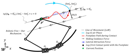
Figure 5.
Proposed walking-in-place control method for the ground stage.
A sliding guidance force is then added to , enabling controlled sliding in the opposite direction of the humanoid robot’s movement. This approach aims to keep the body center stable while the humanoid robot is walking. While the body center can be maintained temporarily, accumulated errors over time cause the midpoint of distance between left and right footholders, and , to progressively move away from the center point . Consequently, the humanoid robot begins to drift outward from the platform’s center. To maintain the midpoint between the footplates at over time, supplementary forces are applied to the centers of each footholder along the x and y axes. To control the drift error represented by and , the error is multiplied by the control coefficient in the Equation (29), thereby compensating for the drift error. was optimized through a trial-and-error approach.
Subsequently, the values are multiplied by the Jacobians provided in Equation (30), yielding the torques to be applied to the O51 and O54 joints in both robotic mechanisms. In this way, as the walking process continues, the midpoint of the footholder separation is simultaneously adjusted at each time step to stay centered at point along the x and y axes. Here, it is known that the position, velocity, and foot angle data for the humanoid robot’s foot points are provided through motion capture and sensor systems. Subsequently, torque mapping to the necessary joints is performed, as specified in Equation (30). As the robotic five-bar mechanisms move around the circular platform and their angles vary, they are multiplied by the rotation matrix to account for these changes.
To ensure that the humanoid robot stays centered on the platform, the value of must be accurately set. This value was optimized using a genetic algorithm. Here, it is desired that the midpoint between the footplates always remain at the symmetrical center of the robotic platform. Therefore, in the genetic optimization algorithm, deviations of the midpoint from the center are penalized, driving the solution to converge on the value that minimizes the error.
In the MATLAB Simulink environment, the humanoid is programmed to walk on the ODT for intervals of s. As it drifts further from the center of the ODT, it receives increasingly higher penalty scores. The genetic algorithm evolves to find the coefficient that best keeps the footplates near the center. The objective function is provided in Equation (31). While determining the coefficient, the value is set to zero to achieve the best result without the influence of the drift error compensator. The optimization update interval is chosen as seconds.
3.3. ODT Footplate Rotation Control
Typically, during walking, we apply a wrench torque to the feet to enable turning while moving on the ground. For the torque to facilitate turning, the angle of the footholder must remain unchanged during the rotation. During walking, the footplate aligns in the direction of rotation, focusing on the combined angle of the humanoid leg . The expression represents the desired reference angle for the footplate. As long as , the value of is equal to at the moment of contact , as shown in Equation (32). It also signifies that remains constant, meaning that it does not change, while .
Given that
where
In Equation (33), it is stated that when , becomes equal to . Thus, the resulting error is used in a PD control to obtain the control torque as described in Equation (34).
3.4. ODT Five-Bar Base Control Around Circular Track
The robotic five-bar is capable of reaching target coordinates by simultaneously adjusting both the arm and the five-bar base with movement and rotation around the circular path. However, to minimize unnecessary movements and reduce control complexity, the system can be optimized by prioritizing five-bar link motion and restricting base movement. Each five-bar mechanism operates within its defined workspace. However, when moves outside the specified workspace, the angle adjusts accordingly to compensate for this deviation. The algorithm proposed to control this situation is provided in Algorithm 1. We know that joint limits are not violated when , where represents the safe workspace of the five-bar robots. Additionally, even within the safe zone, if the angles of the two legs remain equal for a specified period, the positions of the robotic five-bar bases are reconfigured accordingly. When both feet are aligned in the same direction, the values of are determined using the equation provided. The error term , controlled by the PD controller, determines the orientation of both robotic five-bar mechanisms. The difference is controlled using a PD controller, yielding the control torque as presented in Algorithm 1.
| Algorithm 1. Base control around circular track algorithm. |
//: The relevant state variable, initialized to at the beginning. if then if then End End if then if then if then End End End //Violating the limits of the safe workspace if if then End End |
3.5. Dynamic Footholder Collision Avoidance
Since the positions of the robotic end effectors are well-known, a dynamic collision avoidance system can be implemented. While the regions and may intersect, an artificial potential energy-based dynamic collision avoidance algorithm was employed in the case of an intersection between regions and . The repulsive potential energy , which depends on the distance between the robot and the obstacle, is given in Equation (35). is a positive constant that determines the intensity of the repulsive potential. It has been optimized through trial and error. is the distance between the robot’s position and the obstacle. is the distance at which the potential energy is equal to zero.
The force can be calculated as the negative gradient of the potential energy, as shown in Equation (36).
is the unit vector that represents the direction of the repulsive force. Here, the footplate in contact is considered an obstacle. The footplate, which follows the humanoid foot in flight stage, needs to avoid this obstacle. The proposed algorithm for obstacle avoidance is provided in Algorithm 2. Additionally, to prevent the footplates from getting stuck at any point, a new trajectory was derived from the trajectory , and the coefficient was determined through trial and error. Thus, in addition to the repulsive forces, the escape trajectory in front of the footplate’s path ensures the avoidance of obstacles.
| Algorithm 2. Dynamic footholder collision avoidance algorithm. |
begin then end |
Throughout the walking process, the torques applied to the Oi51 and Oi54 joints are given by summing the values in Equation (37). During the simulations, a constraint was applied to the maximum control torque , as specified in Equation (37). The system architecture for the simulation, which includes the humanoid and the robotic ODT, is shown in Figure 6.
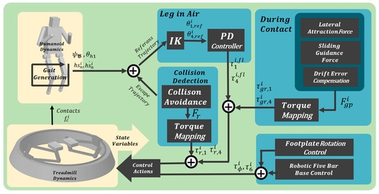
Figure 6.
The proposed complete control framework for the robotic ODT. The architecture integrates multiple state-dependent controllers.
4. Numerical Simulation
To evaluate the performance of the proposed method, two different simulations were conducted on the robotic ODT. The parameters necessary for controlling the robots and the initial values used in the simulations are presented in Table 2.
Table 2.
Parameters for numerical simulation.
In the initial numerical simulation, the humanoid robot performs a specific gait pattern, which also involves turning maneuvers, over a period of 80 s. The same locomotion performed on the flat surface was also replicated on the robotic ODT. Figure 7 presents screenshots captured during the operation of the ODT in the simulation and on a flat surface. Figure 8 (middle graph) shows the tracking graph of the humanoid robot’s body center and foot tip points during locomotion on a flat surface. Additionally, the walking results on the ODT are presented in Figure 8 (left graph). The graph indicates that the body center and feet remained within the boundaries of the ODT platform. Figure 8 (right graph) shows that the midpoint of distance between the two footplates, which coincides with the center point of the ODT, exhibits very small oscillations. Over the entire simulation, the mean resultant drift error was 2.73 cm, with a standard deviation of 2.02 cm, indicating small and consistent oscillations. The maximum resultant drift error was 11.65 cm, a peak value that occurred momentarily during a turning motion and remained well within the ODT’s safe operational boundaries, with peak errors along any single axis remaining below 9 cm. The control effort required to achieve this stability is illustrated in Figure 9 and Figure 10, which show the angular position and torque profiles for the ODT’s actuated joints, respectively. As the humanoid initiated turns by pivoting on its right foot to push off and generate torque for the turning maneuvers, the highest loads were consequently observed on the right-side mechanism. The RMS torques for the most loaded actuators (right side) were 21.54 Nm. These values, derived from a control signal constrained by a ±50 Nm saturation limit, numerically demonstrate that the actuators are sufficiently powerful for the task, with the average load remaining well below the continuous duty capacity of typical motors. The torques responsible for controlling the footholder orientation () were limited to a maximum of 20 Nm. Right RMS torques = [19.7906, 21.5401, 14.0210, 12.8371] Nm, and Left RMS torques = [20.048, 17.53, 14.81, 3.03] Nm are given in order. Furthermore, the power consumption evaluation quantifies the system’s electrical requirements, such as those of the power supply and motor drivers, establishing a total sustained power draw of 260 W and a critical peak demand of 383 W from a single actuator. Finally, Figure 11 provides a detailed view of the tracking performance, confirming that the ODT footplates precisely follow the humanoid’s foot tip trajectories throughout the complex locomotion sequence.
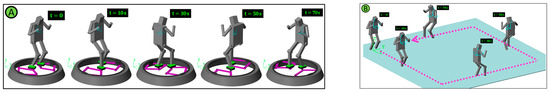
Figure 7.
Dynamic simulation of a humanoid robot walking on an ODT (A) and on a flat surface (B).
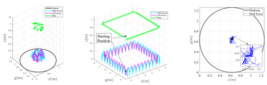
Figure 8.
Humanoid robot base and foot tip tracking on an ODT (left graph) and on a flat surface (middle graph); footholders center drift error (right graph).
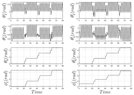
Figure 9.
The graph shows the changes in the angular position of the robotic ODT during walking.
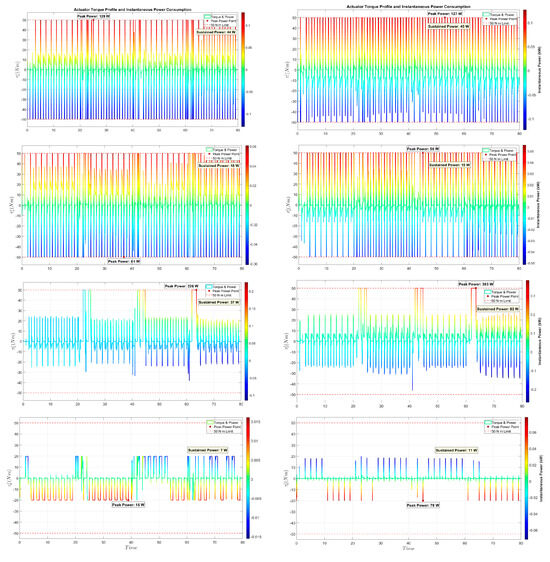
Figure 10.
Torque profiles and power consumption for the robotic ODT during walking. In each subplot, line color maps to power draw (kW), and annotations specify peak/sustained power (W).
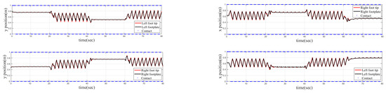
Figure 11.
Foot tip tracking control performance. The plot provides a direct comparison between the desired reference trajectory (red) and the actual trajectory executed by the footplates (black).
4.1. Catwalk Gait ····Robotic ODT
In the second simulation, the humanoid attempts to walk on a straight line, also known as the catwalk gait. Figure 12 presents screenshots captured during the operation of the ODT in the simulation and on a flat surface. This scenario is crucial for evaluating the applicability of the ODT’s footholder dynamic collision avoidance algorithm. Figure 13 (middle graph) shows the tracking graph of the humanoid robot’s body center and foot tip points during catwalking on the flat surface and on the ODT are presented in Figure 13 (left graph). Figure 13 (right graph) shows that the feet remained within the boundaries of the ODT platform and the midpoint of the distance between the two footplates exhibits very small oscillations around center point . These oscillations are within a range of ±9 cm along any single axis.
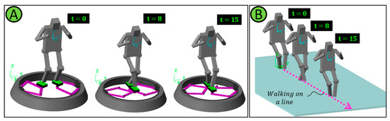
Figure 12.
Dynamic simulation of a humanoid robot catwalking on an ODT (A) and on a flat surface (B).
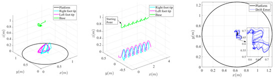
Figure 13.
Humanoid robot base and foot tip tracking during catwalking on an ODT (left graph) and on a flat surface (middle graph); footholders center drift error (right graph).
Analysis of the catwalk gait revealed a mean resultant drift of 5.45 cm, with a standard deviation of 2.70 cm and a maximum of resultant drift error of 11.97 cm. This pronounced lateral deviation is a direct and intended consequence of the collision avoidance algorithm’s operation. Each time the escape logic was triggered to maneuver around an obstacle, it inherently introduced a lateral displacement from the nominal straight path, thereby confirming the system’s ability to prioritize safety over perfect trajectory adherence. Figure 14 shows that the ODT footplates follow the foot tip points throughout locomotion. The graph shows that when an obstacle is detected, the footplates adjust their trajectory to prevent a collision. The angular position and torque-power (kw) graphs obtained from the 15 s control of the ODT are presented in Figure 15 and Figure 16. During the catwalking gait, the system exhibited a total sustained power consumption of 293 W, with the highest drawing primary motor consuming 80 W.
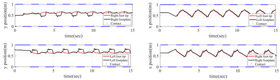
Figure 14.
Foot tip tracking control performance during catwalking. The plot provides a direct comparison between the desired reference trajectory (red) and the actual trajectory executed by the footplates (black). The trajectory modifications implemented to prevent collisions are illustrated in the figures.
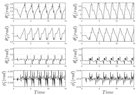
Figure 15.
The graph shows the changes in the angular position of the robotic ODT during catwalking.
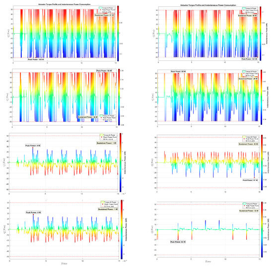
Figure 16.
Torque profiles and power consumption for the robotic ODT during catwalking. In each subplot, line color maps to power draw (kW), and annotations specify peak/sustained power (W).
The footplates have dimensions of 0.20 m × 0.13 m. For the footplates, the safe corner regions () were defined with dimensions of 0.22 m × 0.19 m. The intersection of the regions and is used to evaluate the metric , as described in Algorithm 2. During crossover gait, the avoidance logic was triggered a total of 190 times to maneuver the footplates, with an average minimum distance of 0.22 m and minimum clearance of 0.18 m. Here, it should be noted that the artificial field generated for this avoidance is a circular area. Activation of the Collision Avoidance Logic profile during the Crossover Gait is illustrated in Figure 17 (Right).
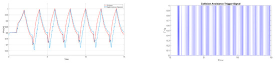
Figure 17.
Execution of the Commanded Escape Trajectory and reference humanoid foot tip for right section (left) reference and (right) activation of the Collision Avoidance Logic during Crossover Gait.
Since the left and right mechanisms exhibited similar behaviors, execution of the Commanded Escape Trajectory and reference humanoid foot tip for the right section are illustrated in Figure 17 (left). The graph illustrates the system’s response to an obstacle. The trajectory deviation was calculated at 17.76%. While this value may appear significant, it is crucial to note that this deviation is an intentional and necessary feature of the control strategy. During the flight phase, this deliberate path modification occurs if the footholder encounters an obstacle while sliding, serving as a preventive measure to prevent a potential collision.
4.2. Robustness Analysis of the Control Architecture
To evaluate the controller’s robustness to measurement inaccuracies, the simulation was performed with zero-mean uniform white noise added to the foot tip position reference signals (), representing position signals obtained from MoCap, IMU, or vision-based sensors. Two noise levels were considered, with peak amplitudes of ±1 mm to represent a high-quality tracking system and ±3 mm to simulate a lower-quality sensor or noisier environment. Furthermore, zero-mean uniform white noise of ±0.05° and ±0.1° was added to all joints of the robotic ODT to model encoder noise, and the system was tested under both levels. The impact of real-world hardware latency was analyzed by adding a transport delay to the foot-tip position feedback loop. Although most modern sensors operate at an update frequency of 100 Hz, the system was tested with latencies of 20 ms and 40 ms to evaluate performance under more adverse conditions. A comprehensive analysis, including a worst-case scenario combining both adverse effects, was conducted, with the quantitative results summarized in Table 3, based on six tests in which the humanoid walked at a , an intermediate heading angle chosen to better observe the effect of the LoM.
Table 3.
Robustness analysis with saturated actuators (Max. 50 Nm limit for and 20 Nm limit for ).
The analysis reveals that the controller exhibits excellent noise rejection capabilities in terms of positioning accuracy. Even under high-amplitude noise conditions (±3 mm position, ±0.1 deg encoder), the maximum resultant drift error increased by a negligible 0.2% compared to the ideal case. However, this high level of accuracy is achieved at the cost of significantly increased control effort. The application of high amplitude noise more than doubled the RMS torque demand on the primary actuator , with a 102.9% increase from 16.629 Nm to 33.75 Nm. This indicates that while the controller successfully filters out noise to maintain user centering, its practical implementation would necessitate actuators capable of handling higher dynamic loads to prevent overheating and ensure longevity, making the selection of high-quality, low-noise sensors a critical design consideration for energy efficiency.
In contrast to sensor noise, the analysis of latency in the feedback loop shows that latency primarily affects the system’s positional tracking precision, with a minimal impact on actuator effort. Applying a hardware latency of 20 ms resulted in a minor 2.6% increase in the maximum resultant drift error. When subjected to a more adverse 40 ms delay, the maximum error increased by 8.1% to 4.52 cm, while the RMS torque values remained nearly identical to the ideal case. This demonstrates that the control system remains robustly stable in the presence of realistic communication delays, although minimizing latency is crucial for achieving the highest degree of centering accuracy.
The final test scenario, combining high-amplitude sensor noise with a 40 ms latency, confirms the distinct effects of these two imperfections. The resulting maximum resultant drift error of 4.55 cm is primarily dictated by the latency-induced phase lag, while the high RMS torque values are almost entirely attributable to the controller’s aggressive compensation for sensor noise. Even under these compounded adverse conditions, the system successfully maintained the user’s center within a tight bound, demonstrating the exceptional robustness and practical viability of the proposed control architecture for real-world applications.
5. Conclusions and Recommendations
The results demonstrate the effectiveness of our human in the loop control framework. By tightly coupling the ODT’s dynamics with the user’s locomotion, we achieved robust stabilization with minimal drift. This HIL approach distinguishes our work from traditional ODTs that often rely on less adaptive, slip-based mechanics, which can compromise the naturalness of the gait. Simulation results for full-turn straight walking indicate a mean resultant drift error of 2.73 cm, with a standard deviation of 2.02 cm, reflecting small and consistent oscillations. The maximum resultant drift error reached 11.65 cm. The RMS torque for the most heavily loaded actuator, , was 21.54 Nm, and the humanoid remained within the ODT’s safe operational boundaries.
Although testing of the robotic ODT has been conducted with a point-contact humanoid model, and its operational principles have been explained, developing a more detailed and realistic dynamic human model is necessary to better understand its strengths and limitations. Alternatively, producing a prototype of the robotic ODT could provide valuable insights into its impact on the human user and its effect on walking comfort, potentially leading to improved outcomes. AI-based control agents can be utilized to address complex human gait models effectively. By training the agent with thousands of different locomotion footstep patterns, more robust controllers can be developed. It is known that robotic five-bar mechanisms can provide haptic feedback. Additionally, vertical movement can be enabled for the ODT’s footplates using basic mechanisms. Thus, the footplates will be able to move according to the height of the meshes in the VR environment. It will even be possible to perform actions such as climbing stairs or jumping on a trampoline.
Funding
This research received no external funding.
Data Availability Statement
Data available on request due to restrictions (privacy).
Acknowledgments
I acknowledge the use of the library and literature resources at Hakkari University for conducting the literature review.
Conflicts of Interest
The author declares no conflicts of interest.
Appendix A

Figure A1.
Main control structures and dynamic models for humanoid and robotic ODT.
Figure A1.
Main control structures and dynamic models for humanoid and robotic ODT.


Figure A2.
Humanoid robot subsystem.
Figure A2.
Humanoid robot subsystem.


Figure A3.
Dynamic models of the right footplate.
Figure A3.
Dynamic models of the right footplate.


Figure A4.
Five-bar planar mechanism collision-free link configuration.
Figure A4.
Five-bar planar mechanism collision-free link configuration.

References
- Martinez, E.S.; Wu, A.S.; McMahan, R.P. Research Trends in Virtual Reality Locomotion Techniques. In Proceedings of the 2022 IEEE Conference on Virtual Reality and 3D User Interfaces, VR 2022, Christchurch, New Zealand, 12–16 March 2022; pp. 270–280. [Google Scholar] [CrossRef]
- Warren, L.E.; Bowman, D.A. User experience with semi-natural locomotion techniques in virtual reality: The case of the virtuix omni. In Proceedings of the SUI 2017—Proceedings of the 2017 Symposium on Spatial User Interaction, Brighton, UK, 16–17 October 2017; p. 163. [Google Scholar] [CrossRef]
- Pyo, S.; Lee, H.; Yoon, J. Development of a novel omnidirectional treadmill-based locomotion interface device with running capability. Appl. Sci. 2021, 11, 4223. [Google Scholar] [CrossRef]
- Wang, Z.; Liu, C.; Chen, J.; Yao, Y.; Fang, D.; Shi, Z.; Yan, R.; Wang, Y.; Zhang, K.; Wang, H.; et al. Strolling in Room-Scale VR: Hex-Core-MK1 Omnidirectional Treadmill. IEEE Trans. Vis. Comput. Graph. 2023, 29, 5538–5555. [Google Scholar] [CrossRef] [PubMed]
- Bashir, A.; De Regt, T.; Jones, C.M. Comparing a friction-based uni-directional treadmill and a slip-style omni-directional treadmill on first-time HMD-VR user task performance, cybersickness, postural sway, posture angle, ease of use, enjoyment, and effort. Int. J. Hum. Comput. Stud. 2023, 179, 103101. [Google Scholar] [CrossRef]
- Mousas, C.; Kao, D.; Koilias, A.; Rekabdar, B. Evaluating virtual reality locomotion interfaces on collision avoidance task with a virtual character. Vis. Comput. 2021, 37, 2823–2839. [Google Scholar] [CrossRef]
- Hooks, K.; Ferguson, W.; Morillo, P.; Cruz-Neira, C. Evaluating the user experience of omnidirectional VR walking simulators. Entertain. Comput. 2020, 34, 100352. [Google Scholar] [CrossRef]
- Otaran, A.; Farkhatdinov, I. Haptic Ankle Platform for Interactive Walking in Virtual Reality. IEEE Trans. Vis. Comput. Graph. 2022, 28, 3974–3985. [Google Scholar] [CrossRef]
- Kim, W.; Sung, J.; Xiong, S. Walking-in-place for omnidirectional VR locomotion using a single RGB camera. Virtual Real. 2022, 26, 173–186. [Google Scholar] [CrossRef]
- Choi, Y.; Park, D.-H.; Lee, S.; Han, I.; Akan, E.; Jeon, H.-C.; Luo, Y.; Kim, S.; Matusik, W.; Rus, D.; et al. Seamless-walk: Natural and comfortable virtual reality locomotion method with a high-resolution tactile sensor. Virtual Real. 2023, 27, 1431–1445. [Google Scholar] [CrossRef]
- Sra, M.; Jain, A.; Maes, P. Adding Proprioceptive Feedback to Virtual Reality Experiences Using Galvanic Vestibular Stimulation. In Proceedings of the CHI ’19: 2019 CHI Conference on Human Factors in Computing Systems, Glasgow Scotland, UK, 4–9 May 2019; pp. 1–14. [Google Scholar] [CrossRef]
- Hwang, S.; Lee, J.; Kim, Y.I.; Kim, S.J. REVES: Redirection Enhancement Using Four-Pole Vestibular Electrode Stimulation. In Proceedings of the Conference on Human Factors in Computing Systems, New Orleans, LA, USA, 29 April–5 May 2022. [Google Scholar] [CrossRef]
- Zenner, A.; Karr, C.; Feick, M.; Ariza, O.; Krüger, A. Beyond the Blink: Investigating Combined Saccadic & Blink-Suppressed Hand Redirection in Virtual Reality. In Proceedings of the Conference on Human Factors in Computing Systems, Honolulu, HI, USA, 11–16 May 2024. [Google Scholar] [CrossRef]
- Sun, Q.; Patney, A.; Wei, L.-Y.; Shapira, O.; Lu, J.; Asente, P.; Zhu, S.; Mcguire, M.; Luebke, D.; Kaufman, A. Towards virtual reality infinite walking: Dynamic saccadic redirection. ACM Trans. Graph. 2018, 37, 1–13. [Google Scholar] [CrossRef]
- Groth, C.; Tauscher, J.P.; Heesen, N.; Hattenbach, M.; Castillo, S.; Magnor, M. Omnidirectional Galvanic Vestibular Stimulation in Virtual Reality. IEEE Trans. Vis. Comput. Graph. 2022, 28, 2234–2244. [Google Scholar] [CrossRef] [PubMed]
- Su, J.; Li, S.; Hu, B.; Yin, L.; Zhou, C.; Wang, H.; Hou, S. Innovative insights into nanofluid-enhanced gear lubrication: Computational and experimental analysis of churn mechanisms. Tribol. Int. 2024, 199, 109949. [Google Scholar] [CrossRef]
- Su, J.; Ouyang, Y.; Yin, L.; Shi, Z.; Zhou, C.; Wang, H.; Hu, B. Advancing wind turbine gearbox durability with eco-friendly GO nanolubricants: CFD simulation–experiment synergy for understanding flow dynamics, wear suppression and surface restoration mechanisms. Tribol. Int. 2025, 213, 111034. [Google Scholar] [CrossRef]
- Nguyen, H.X.; Cao, H.Q.; Nguyen, T.T.; Tran, T.N.C.; Tran, H.N.; Jeon, J.W. Improving Robot Precision Positioning Using a Neural Network Based on Levenberg Marquardt-APSO Algorithm. IEEE Access 2021, 9, 75415–75425. [Google Scholar] [CrossRef]
- Yan, S.; Wang, Z.; Zhu, Z.; Ding, J.; Zhang, W.; Zhang, K.; Wei, H. Human Gait Detection Method Based on Binocular Vision for Virtual Reality Omnidirectional Treadmill. In Proceedings of the 36th Chinese Control and Decision Conference, CCDC 2024, Xi’an, China, 25–27 May 2024; pp. 1995–2002. [Google Scholar] [CrossRef]
- Chavdarov, I. Kinematics and Force Analysis of a Five-Link Mechanism by the Four Spaces Jacoby Matrix. [Online]. Available online: https://www.researchgate.net/publication/290393600 (accessed on 14 June 2025).
- Roscia, F.; Cumerlotti, A.; Del Prete, A.; Semini, C.; Focchi, M. Orientation Control System: Enhancing Aerial Maneuvers for Quadruped Robots. Sensors 2023, 23, 1234. [Google Scholar] [CrossRef] [PubMed]
- Lee, C.-Y.; Yang, S.; Bokser, B.; Manchester, Z. Enhanced Balance for Legged Robots Using Reaction Wheels. In Proceedings of the 2023 IEEE International Conference on Robotics and Automation (ICRA), London, UK, 29 May–2 June 2023; pp. 9980–9987. [Google Scholar] [CrossRef]


Disclaimer/Publisher’s Note: The statements, opinions and data contained in all publications are solely those of the individual author(s) and contributor(s) and not of MDPI and/or the editor(s). MDPI and/or the editor(s) disclaim responsibility for any injury to people or property resulting from any ideas, methods, instructions or products referred to in the content. |
© 2025 by the author. Licensee MDPI, Basel, Switzerland. This article is an open access article distributed under the terms and conditions of the Creative Commons Attribution (CC BY) license (https://creativecommons.org/licenses/by/4.0/).