Exact Solutions to Multiple-Delayed Linear Discrete Matrix Equations

Abstract

This work investigates a new category of linear non-homogeneous discrete-matrix equations that feature multiple delays and first-order differences, under the assumption of pairwise permutable coefficient matrices. We define a novel multi-delayed discrete-matrix-exponential function that extends previous concepts. Using this function and specific commutativity properties, we construct an explicit matrix solution. The study highlights the advantages of our approach by contrasting it with prior research and identifying new open questions. Finally, a numerical example illustrates the application and relevance of the derived solution.

1. Introduction

The study of delayed discrete equations occupies a central role in multiple disciplines. These equations, where a system’s present state depends on its recent history and multiple past states, arise naturally in diverse areas. Their theoretical and practical significance is evident in fields such as stability theory [1,2,3], control theory [4,5,6,7,8], and modeling of dynamical systems [9]. Further applications are found in signal processing [10] and in networked systems analysis [11]. The study of multi-delayed discrete-matrix equations extends beyond theoretical interest and finds substantial applications across various engineering domains. For control systems, such equations naturally arise in networked control systems where multiple communication channels introduce distinct delays between sensors, controllers, and actuators. They are equally crucial in iterative learning control for systems that execute repetitive tasks under varying delay conditions. For signal processing, these equations model multi-rate digital filters and adaptive filtering systems where multiple delayed signal versions are processed concurrently. Furthermore, for networked and distributed systems, multi-delay dynamics are inherent in consensus algorithms and multi-agent coordination problems, where information exchange between agents suffers from heterogeneous communication delays. The explicit solution framework developed in this work provides a foundational tool for analyzing stability, designing controllers, and predicting system behavior in these practical scenarios, thereby bridging a critical gap between theoretical mathematics and engineering applications. Matrix formulations enable the modeling of multi-variable systems, thereby directly addressing complex, real-world challenges in engineering and science.

Obtaining explicit or closed-form solutions provides deep insight into the behavior of the system and enables the precise characterization of key dynamical properties. Moreover, the solutions to initial value problems for linear discrete delayed systems is effectively addressed through delayed discrete-matrix functions, as they offer a compact matrix formulation that fully encapsulates the underlying dynamics. The study of discrete systems with first-order differences has evolved significantly. Initial work by Diblík [12,13,14] focused on equations with a single delay, later extending to systems with two delays under the assumption of commutative coefficient matrices [15,16]. This line of inquiry was generalized by Medved’ and Pospisil [17,18], who considered systems with several delays and pairwise commutative matrices. Subsequently, Jin and Mahmudov [19,20,21] broadened the framework further by developing solutions that do not require commutativity conditions, thereby encompassing non-commutative matrix coefficients. A comprehensive summary of existing results in this area is provided by the recent survey [22]. The foundational framework established therein has been instrumental in driving major advances across several domains, including stability analysis [1,23,24], iterative learning control [4,19,25,26], and problems of relative controllability [8,27].

A recent contribution by Diblík [12] was the introduction of a new class of discrete-matrix equations featuring a single delay and a first-order forward difference, for which he established an explicit solution representation:

$$\Delta \mathbb{Y}\left(k\right)=\mathbb{M}\mathbb{Y}\left(k-\varkappa \right)+\mathbb{Y}\left(k-\varkappa \right)\mathbb{H}+\Lambda \left(k\right),$$

(1)

where the independent variable k is in ${\mathcal{Z}}_0^{\infty }$, defined for integers $p\le q$ as the set $\{k\in \mathbb{Z}:p\le k\le q\}$, with infinite limits allowed. In Equation (1), $\varkappa >0$ is the delay. The unknown matrix function $\mathbb{Y}$ maps ${\mathcal{Z}}_{-\varkappa }^{\infty }$ to ${\mathbb{R}}^{n\times n}$, while $\Lambda :{\mathcal{Z}}_0^{\infty }\to {\mathbb{R}}^{n\times n}$ is a known function. The first-order forward-difference operator is given by

$$\Delta \mathbb{Y}\left(k\right)=\mathbb{Y}(k+1)-\mathbb{Y}\left(k\right),$$

and $\mathbb{M},\mathbb{H}\in {\mathbb{R}}^{n\times n}$ are constant matrices.

We address two key objectives motivated by Diblík’s work [12]. First, we provide affirmative solutions to the open problems of extending the theory to multiple delays for both permutable and non-permutable matrices. Second, we achieve this by investigating a novel class of matrix equations of the form

$$\left\{\begin{array}{c}\Delta \mathbb{Y}\left(k\right)={\displaystyle \sum _{i=1}^d}\left[{\mathbb{M}}_i\mathbb{Y}\left(k-{\varkappa }_i\right)+\mathbb{Y}\left(k-{\varkappa }_i\right){\mathbb{H}}_i\right]+\Lambda \left(k\right),\mathrm{for}k\in {\mathbb{Z}}_0^{\infty },\\ \mathbb{Y}\left(k\right)=\Psi \left(k\right),\mathrm{for}k\in {\mathbb{Z}}_{-\varkappa }^0,\end{array}\right.$$

(2)

that feature these multiple delays and first-order forward differences, for which we construct exact solutions, where ${\varkappa }_i\in \mathbb{N}={\mathbb{Z}}_1^{\infty }$ are the delay parameters for $i=1,\dots ,d$, and $\varkappa :=max\{{\varkappa }_1,\dots ,{\varkappa }_d\}$. The function $\mathbb{Y}:{\mathcal{Z}}_{-\varkappa }^{\infty }\to {\mathbb{R}}^{n\times n}$ denotes the unknown matrix-valued function satisfying (2) for all $k\in {\mathbb{Z}}_0^{\infty }$. The system is defined by the coefficient sequences $\mathbb{M}=({\mathbb{M}}_1,{\mathbb{M}}_2,\dots ,{\mathbb{M}}_d)$ and $\mathbb{H}=({\mathbb{H}}_1,{\mathbb{H}}_2,\dots ,{\mathbb{H}}_d)$, where each ${\mathbb{M}}_i,{\mathbb{H}}_i\in {\mathbb{R}}^{n\times n}$ is a given nonzero constant matrix. The dynamics are driven by a given inhomogeneous term $\Lambda :{\mathcal{Z}}_0^{\infty }\to {\mathbb{R}}^{n\times n}$ and a prescribed initial function $\Psi :{\mathcal{Z}}_{-\varkappa }^0\to {\mathbb{R}}^{n\times n}$.

The paper is organized in the following manner: We begin in Section 2 by establishing foundational definitions and presenting a newly developed multi-delayed discrete-matrix-exponential function, detailing its critical properties. The primary contribution of this work is contained in Section 3, where we leverage this function to construct an explicit solution for problem (2). To conclude, Section 4 provides an illustrative example supported by numerical simulations that corroborate the established theory.

2. Preliminaries

This section presents the preliminary concepts of multi-delayed discrete-matrix functions and discrete calculus that are essential for the subsequent calculations. The following notation will be adopted:

• For integers $r\le s$, the discrete interval is defined as ${\mathbb{Z}}_r^s=\{r,r+1,\dots ,s\}$. According to convention, ${\mathbb{Z}}_r^s=\varnothing$ if $r>s$.
• The infinite discrete interval is given by ${\mathbb{Z}}_r^{\infty }=\{r,r+1,\dots \}$.

In addition, let $\mathbf{E}$ and $\mathbf{0}$ denote the $n\times n$ identity and zero matrices, respectively. We adhere to the standard conventions for empty sums and products: for any sequence,

$$\sum _{i=s_1}^{s_2}(\cdots )=\mathbf{0}\mathrm{and}\prod _{i=s_1}^{s_2}(\cdots )=\mathbf{E}\mathrm{whenever}{s}_1>s_2.$$

For scalars, the empty sum is 0 and the empty product is 1. Moreover, the binomial coefficient is defined for integers a and b by

$$\left({\displaystyle \genfrac{}{}{0pt}{}{a}{b}}\right):=\left\{\begin{array}{cc}{\displaystyle \frac{a!}{b!(a-b)!}},\hfill & \mathrm{if}0\le b\le a,\hfill \\ 0,\hfill & \mathrm{otherwise},\hfill \end{array}\right.$$

with the convention $0!=1$. These coefficients satisfy the following fundamental identities for integers $a,b$:

$$\begin{array}{cc}\hfill \left({\displaystyle \genfrac{}{}{0pt}{}{a+1}{b}}\right)& =\left({\displaystyle \genfrac{}{}{0pt}{}{a}{b}}\right)+\left({\displaystyle \genfrac{}{}{0pt}{}{a}{b-1}}\right),\hfill \\ \hfill \left({\displaystyle \genfrac{}{}{0pt}{}{a}{a}}\right)& =\left({\displaystyle \genfrac{}{}{0pt}{}{a-1}{a-1}}\right),\hfill \\ \hfill \left({\displaystyle \genfrac{}{}{0pt}{}{a}{0}}\right)& =\left({\displaystyle \genfrac{}{}{0pt}{}{a-1}{0}}\right).\hfill \end{array}$$

Finally, for a positive integer n and non-negative integers $m_1,m_2,\dots ,m_n$ such that $M={\sum }_{j=1}^n{m}_j$, the multinomial coefficient is defined as

$$\left({\displaystyle \genfrac{}{}{0pt}{}{M}{m_1,m_2,\dots ,m_n}}\right)={\displaystyle \frac{M!}{{\prod }_{j=1}^n{m}_j!}}.$$

Lemma 1 

([28]). Let $n_1,n_2\in \mathbb{Z}$ such that $n_1<n_2$. For any functions u and v, the following identities are satisfied:

$${\Delta }_{k}u\left(k,r\right):=u\left(k+1,r\right)-u\left(k,r\right),$$

$$\sum _{r=n_1}^{n_2}u\left(r\right)\Delta v\left(r\right)=u\left(n_2\right)v\left(n_2+1\right)-u\left(n_1\right)v\left(n_1\right)-\sum _{r=n_1+1}^{n_2}\Delta u\left(r-1\right)v\left(r\right),$$

$${\Delta }_k\left[\sum _{r=1}^{k}u\left(k,r\right)\right]=u\left(k+1,k+1\right)+\sum _{r=1}^k{\Delta }_{k}u\left(k,r\right).$$

Definition 1. 

Let $\mathbb{M}$ $=\left({\mathbb{M}}_1,\dots ,{\mathbb{M}}_d\right)$ and $\mathbb{H}$ $=\left({\mathbb{H}}_1,\dots ,{\mathbb{H}}_d\right)$ be $n\times n$ constant real nonzero matrices. We introduce the determining matrix equation ${\mathsf{\text{ϝ}}}^{\mathbb{M},\mathbb{H}}(k;\tau )\in {\mathbb{R}}^{n\times n}$ of the form

$${\mathsf{\text{ϝ}}}^{\mathbb{M},\mathbb{H}}(k+1;\tau )={\displaystyle \sum _{j=1}^d}[{\mathbb{M}}_j{\mathsf{\text{ϝ}}}^{\mathbb{M},\mathbb{H}}(k;\tau -{\mathbf{e}}_j)+{\mathsf{\text{ϝ}}}^{\mathbb{M},\mathbb{H}}(k;\tau -{\mathbf{e}}_j){\mathbb{H}}_j],\mathit{for}k\in {\mathbb{Z}}_0^{\infty },\tau \in {\left({\mathbb{Z}}_0^{\infty }\right)}^d,$$

(3)

such that

$$\begin{array}{cc}\hfill & {\mathsf{\text{ϝ}}}^{\mathbb{M},\mathbb{H}}(0;\tau )=\Theta ,{\mathsf{\text{ϝ}}}^{\mathbb{M},\mathbb{H}}(1;0)=\mathbb{E},\hfill \\ \hfill & {\mathsf{\text{ϝ}}}^{\mathbb{M},\mathbb{H}}(k;-1,{\tau }_2,\dots ,{\tau }_d)={\mathsf{\text{ϝ}}}^{\mathbb{M},\mathbb{H}}(k;{\tau }_1,-1,\dots ,{\tau }_d)=\cdots ={\mathsf{\text{ϝ}}}^{\mathbb{M},\mathbb{H}}(k;{\tau }_1,{\tau }_2,\dots ,-1)=\Theta ,\hfill \end{array}$$

where ${\mathbf{e}}_j$, $j=1,\dots ,d$ is the canonical basis of ${\mathbb{R}}^d$.

Lemma 2. 

For $k\in {\mathbb{Z}}_0^{\infty }$ and ${\tau }_1+{\tau }_2+\cdots +{\tau }_d\ge k+1$, we have ${\mathsf{\text{ϝ}}}^{\mathbb{M},\mathbb{H}}(k+1;\tau )=\Theta .$

Proof. 

According to Definition 1,

$$\begin{array}{cc}\hfill & {\mathsf{\text{ϝ}}}^{\mathbb{M},\mathbb{H}}(1;\tau )={\displaystyle \sum _{j=1}^d}[{\mathbb{M}}_j{\mathsf{\text{ϝ}}}^{\mathbb{M},\mathbb{H}}(0;\tau -{\mathbf{e}}_j)+{\mathsf{\text{ϝ}}}^{\mathbb{M},\mathbb{H}}(0;\tau -{\mathbf{e}}_j){\mathbb{H}}_j]\hfill \\ \hfill & =\Theta ,\mathrm{for}{\tau }_1+{\tau }_2+\cdots +{\tau }_d\ge 1.\hfill \end{array}$$

According to mathematical induction, if ${\mathsf{\text{ϝ}}}^{\mathbb{M},\mathbb{H}}(n;\tau )=\Theta$, for ${\tau }_1+{\tau }_2+\cdots +{\tau }_d\ge n$, then we get

$$\begin{array}{cc}\hfill {\mathsf{\text{ϝ}}}^{\mathbb{M},\mathbb{H}}(n+1;\tau )& ={\displaystyle \sum _{j=1}^d}[{\mathbb{M}}_j{\mathsf{\text{ϝ}}}^{\mathbb{M},\mathbb{H}}(n;\tau -{\mathbf{e}}_j)+{\mathsf{\text{ϝ}}}^{\mathbb{M},\mathbb{H}}(n;\tau -{\mathbf{e}}_j){\mathbb{H}}_j]\hfill \\ \hfill & =\Theta ,\mathrm{for}{\tau }_1+{\tau }_2+\cdots +{\tau }_d-1\ge n.\hfill \end{array}$$

The proof is complete. □

Definition 2. 

The multi-delayed discrete-matrix exponential ${\mathcal{E}}^{\mathbb{M},\mathbb{H}}\left(k\right)$ is defined as follows:

$${\mathcal{E}}^{\mathbb{M},\mathbb{H}}\left(k\right)={\displaystyle \sum _{\begin{array}{c}{\rho }_1,\dots ,{\rho }_d\ge 0\\ {\sum }_{q=1}^d{\varkappa }_q{\rho }_q+\vartheta \le k\end{array}}}\left({\displaystyle \genfrac{}{}{0pt}{}{k-{\sum }_{q=1}^d{\varkappa }_q{\rho }_q}{{\rho }_1,{\rho }_2,\dots ,{\rho }_d,k-{\sum }_{q=1}^d{\varkappa }_q{\rho }_q-\vartheta }}\right){\mathsf{\text{ϝ}}}^{\mathbb{M},\mathbb{H}}(\vartheta +1;\rho ),$$

(4)

for any $k\in {\mathbb{Z}}_{-\varkappa }^{\infty }$, $\rho =\left({\rho }_1,{\rho }_2,\dots ,{\rho }_d\right)$, $\vartheta ={\sum }_{i=1}^d{\rho }_i$, and ${\mathsf{\text{ϝ}}}^{\mathbb{M},\mathbb{H}}(\vartheta +1;\rho )$ is given by (3).

Lemma 3. 

Given the sequences of $n\times n$ constant real nonzero matrices $\mathbf{S}=({\mathbb{M}}_1,\dots ,{\mathbb{M}}_d)$ and $\mathbf{T}=({\mathbb{H}}_1,\dots ,{\mathbb{H}}_d)$, the multi-delayed matrix function ${\mathcal{E}}^{\mathbf{S},\mathbf{T}}\left(k\right)$ is a solution to the following equation:

$$\Delta {\mathcal{E}}^{\mathbb{M},\mathbb{H}}\left(k\right)={\displaystyle \sum _{i=1}^d}[{\mathbb{M}}_i{\mathcal{E}}^{\mathbb{M},\mathbb{H}}\left(k-{\varkappa }_i\right)+{\mathcal{E}}^{\mathbb{M},\mathbb{H}}\left(k-{\varkappa }_i\right){\mathbb{H}}_i].$$

Proof. 

As a consequence of the definition of ${\mathsf{\text{ϝ}}}^{\mathbb{M},\mathbb{H}}(\vartheta +1;\rho )$, we obtain

$$\begin{array}{cc}\Delta {\mathcal{E}}^{\mathbb{M},\mathbb{H}}\left(k\right)\hfill & ={\mathcal{E}}^{\mathbb{M},\mathbb{H}}\left(k+1\right)-{\mathcal{E}}^{\mathbb{M},\mathbb{H}}\left(k\right)\hfill \\ \hfill & ={\displaystyle \sum _{\begin{array}{c}{\rho }_1,\dots ,{\rho }_d\ge 0\\ {\sum }_{q=1}^d{\varkappa }_q{\rho }_q+\vartheta \le k+1\end{array}}}\left[\left({\displaystyle \genfrac{}{}{0pt}{}{k+1-{\sum }_{q=1}^d{\varkappa }_q{\rho }_q}{{\rho }_1,{\rho }_2,\dots ,{\rho }_d,k+1-{\sum }_{q=1}^d{\varkappa }_q{\rho }_q-\vartheta }}\right)\right.\hfill \\ \hfill & \left.-\left({\displaystyle \genfrac{}{}{0pt}{}{k-{\sum }_{q=1}^d{\varkappa }_q{\rho }_q}{{\rho }_1,{\rho }_2,\dots ,{\rho }_d,k-{\sum }_{q=1}^d{\varkappa }_q{\rho }_q-\vartheta }}\right)\right]{\mathsf{\text{ϝ}}}^{\mathbb{M},\mathbb{H}}(\vartheta +1;\rho )\hfill \\ \hfill & ={\displaystyle \sum _{\begin{array}{c}{\rho }_1,\dots ,{\rho }_d\ge 1\\ {\sum }_{q=1}^d{\varkappa }_q{\rho }_q+\vartheta \le k\end{array}}}\left({\displaystyle \genfrac{}{}{0pt}{}{k-{\sum }_{q=1}^d{\varkappa }_q{\rho }_q}{{\rho }_1,{\rho }_2,\dots ,{\rho }_d,k-{\sum }_{q=1}^d{\varkappa }_q{\rho }_q-\vartheta +1}}\right){\mathsf{\text{ϝ}}}^{\mathbb{M},\mathbb{H}}(\vartheta +1;\rho )\hfill \\ \hfill & ={\displaystyle \sum _{\begin{array}{c}{\rho }_1,\dots ,{\rho }_d\ge 1\\ {\sum }_{q=1}^d{\varkappa }_q{\rho }_q+\vartheta \le k\end{array}}}\left({\displaystyle \genfrac{}{}{0pt}{}{k-{\sum }_{q=1}^d{\varkappa }_q{\rho }_q}{{\rho }_1,{\rho }_2,\dots ,{\rho }_d,k-{\sum }_{q=1}^d{\varkappa }_q{\rho }_q-\vartheta +1}}\right)\hfill \\ \hfill & \times {\displaystyle \sum _{j=1}^d}[{\mathbb{M}}_j{\mathsf{\text{ϝ}}}^{\mathbb{M},\mathbb{H}}(\vartheta ;\rho -{\mathbf{e}}_j)+{\mathsf{\text{ϝ}}}^{\mathbb{M},\mathbb{H}}(\vartheta ;\rho -{\mathbf{e}}_j){\mathbb{H}}_j]\hfill \\ \hfill & ={\displaystyle \sum _{\begin{array}{c}{\rho }_1^{\prime },\dots ,{\rho }_d^{\prime }\ge 0\\ {\sum }_{q=1}^d{\varkappa }_q{\rho }_q^{\prime }+\vartheta \le k-{\varkappa }_j\end{array}}}\left({\displaystyle \genfrac{}{}{0pt}{}{k-{\varkappa }_j-{\sum }_{q=1}^d{\varkappa }_q{\rho }_q^{\prime }}{{\rho }_1^{\prime },{\rho }_2^{\prime },\dots ,{\rho }_d^{\prime },k-{\sum }_{q=1}^d{\varkappa }_q{\rho }_q^{\prime }-{\vartheta }^{\prime }}}\right)\hfill \\ \hfill & \times {\displaystyle \sum _{j=1}^d}[{\mathbb{M}}_j{\mathsf{\text{ϝ}}}^{\mathbb{M},\mathbb{H}}({\vartheta }^{\prime }+1;{\rho }^{\prime })+{\mathsf{\text{ϝ}}}^{\mathbb{M},\mathbb{H}}({\vartheta }^{\prime }+1;{\rho }^{\prime }){\mathbb{H}}_j]\hfill \\ \hfill & ={\displaystyle \sum _{i=1}^d}[{\mathbb{M}}_i{\mathcal{E}}^{\mathbb{M},\mathbb{H}}\left(k-{\varkappa }_i\right)+{\mathcal{E}}^{\mathbb{M},\mathbb{H}}\left(k-{\varkappa }_i\right){\mathbb{H}}_i].\hfill \end{array}$$

This completes the proof. □

3. Solution Structure for Linear Systems with Multiple Delays

We now construct a solution to problem (2) based on the multi-delayed discrete-matrix-exponential function introduced in Definition 2.

Theorem 1. 

Let ${\varkappa }_{\ell }\ge 1$ for $\ell \in \left\{0,1,\dots ,d\right\}$, $\varkappa :=max\left\{{\varkappa }_1,\dots ,{\varkappa }_d\right\}$. Suppose that $\mathbb{M}$ $=\left({\mathbb{M}}_1,\dots ,{\mathbb{M}}_d\right)$, $\mathbb{H}$ $=\left({\mathbb{H}}_1,\dots ,{\mathbb{H}}_d\right)$ are $n\times n$ permutable constant real nonzero matrices; $\Phi \left(k\right){\mathbb{H}}_{\ell }={\mathbb{H}}_{\ell }\Phi \left(k\right)$, for $k\in {\mathbb{Z}}_{-\varkappa }^0$; and ${\mathbb{H}}_{\ell }G\left(k\right)=G\left(k\right){\mathbb{H}}_{\ell }$. Then the solution $\mathbb{Y}\left(k\right)$ to (2) has the form

$$\mathbb{Y}\left(k\right)=\left\{\begin{array}{c}\Phi \left(k\right),k\in {\mathbb{Z}}_{-\varkappa }^0,\hfill \\ {\mathcal{E}}^{\mathbb{M},\mathbb{H}}\left(k\right)\Phi \left(0\right)\hfill \\ +{\displaystyle \sum _{r=1}^d}{\displaystyle \sum _{i=-{\varkappa }_r+1}^0}\left[{\mathbb{M}}_r{\mathcal{E}}^{\mathbb{M},\mathbb{H}}\left(k-{\varkappa }_r-i\right)+{\mathcal{E}}^{\mathbb{M},\mathbb{H}}\left(k-{\varkappa }_r-i\right){\mathbb{H}}_r\right]\Phi \left(i-1\right)\hfill \\ +{\displaystyle \sum _{j=1}^k}{\mathcal{E}}^{\mathbb{M},\mathbb{H}}\left(k-j\right)\Lambda \left(j-1\right),k\in {\mathbb{Z}}_0^{\infty }.\hfill \end{array}\right.$$

(5)

Proof. 

Assume that $k\in {\mathbb{Z}}_0^{\infty }$ is fixed and arbitrary. We prove that $\mathbb{Y}\left(k\right)$ of (5) solves (2). First, if ${\varkappa }_{r_1}\le k<{\varkappa }_{r_2}$ for each $r_1\in {\varkappa }_1$, $r_2\in {\varkappa }_2$ such that ${\varkappa }_1$, ${\varkappa }_2\subset \left\{1,2,\dots ,d\right\}$, then

$${\mathcal{E}}^{\mathbb{M},\mathbb{H}}\left(k-{\varkappa }_{r_2}-i\right)=\left\{\begin{array}{c}{\mathcal{E}}^{\mathbb{M},\mathbb{H}}\left(k-{\varkappa }_{r_2}-i\right),i\in {\mathbb{Z}}_{-{\varkappa }_{r_2}+1}^{k-{\varkappa }_{r_2}},\hfill \\ \Theta ,i\in {\mathbb{Z}}_{k-{\varkappa }_{r_2}+1}^0,\hfill \end{array}\right.$$

and

$$\begin{array}{c}\mathbb{Y}\left(k\right)\hfill \\ ={\mathcal{E}}^{\mathbb{M},\mathbb{H}}\left(k\right)\Phi \left(0\right)\hfill \\ +{\displaystyle \sum _{r_1\in {\varkappa }_1}}{\displaystyle \sum _{i=-{\varkappa }_{r_1}+1}^0}\left[{\mathbb{M}}_{r_1}{\mathcal{E}}^{\mathbb{M},\mathbb{H}}\left(k-{\varkappa }_{r_1}-i\right)+{\mathcal{E}}^{\mathbb{M},\mathbb{H}}\left(k-{\varkappa }_{r_1}-i\right){\mathbb{H}}_{r_1}\right]\Phi \left(i-1\right)\hfill \\ +{\displaystyle \sum _{r_2\in {\varkappa }_2}}{\displaystyle \sum _{i=-{\varkappa }_{r_2}+1}^{k-{\varkappa }_{r_2}}}\left[{\mathbb{M}}_{r_2}{\mathcal{E}}^{\mathbb{M},\mathbb{H}}\left(k-{\varkappa }_{r_2}-i\right)+{\mathcal{E}}^{\mathbb{M},\mathbb{H}}\left(k-{\varkappa }_{r_2}-i\right){\mathbb{H}}_{r_2}\right]\Phi \left(i-1\right)\hfill \\ +{\displaystyle \sum _{j=1}^k}{\mathcal{E}}^{\mathbb{M},\mathbb{H}}\left(k-j\right)\Lambda \left(j-1\right).\hfill \end{array}$$

(6)

Applying the first forward-difference operator to (6) and invoking Lemma 3 results in

$$\begin{array}{cc}\hfill & \Delta \mathbb{Y}\left(k\right)\hfill \\ \hfill & =\Delta {\mathcal{E}}^{\mathbb{M},\mathbb{H}}\left(k\right)\Phi \left(0\right)\hfill \\ \hfill & +{\displaystyle \sum _{r_1\in {\varkappa }_1}}{\displaystyle \sum _{i=-{\varkappa }_{r_1}+1}^0}\left[{\mathbb{M}}_{r_1}\Delta {\mathcal{E}}^{\mathbb{M},\mathbb{H}}\left(k-{\varkappa }_{r_1}-i\right)\Phi \left(i-1\right)\right.\hfill \\ \hfill & \left.+\Delta {\mathcal{E}}^{\mathbb{M},\mathbb{H}}\left(k-{\varkappa }_{r_1}-i\right){\mathbb{H}}_{r_1}\Phi \left(i-1\right)\right]\hfill \\ \hfill & +{\displaystyle \sum _{r_2\in {\varkappa }_2}}{\displaystyle \sum _{i=-{\varkappa }_{r_2}+1}^{k-{\varkappa }_{r_2}}}\left[{\mathbb{M}}_{r_2}\Delta {\mathcal{E}}^{\mathbb{M},\mathbb{H}}\left(k-{\varkappa }_{r_2}-i\right)\Phi \left(i-1\right)\right.\hfill \\ \hfill & \left.+\Delta {\mathcal{E}}^{\mathbb{M},\mathbb{H}}\left(k-{\varkappa }_{r_2}-i\right){\mathbb{H}}_{r_2}\Phi \left(i-1\right)\right]\hfill \\ \hfill & +{\displaystyle \sum _{r_2\in {\varkappa }_2}}\left[{\mathbb{M}}_{r_2}\Phi \left(k-{\varkappa }_{r_2}\right)+\Phi \left(k-{\varkappa }_{r_2}\right){\mathbb{H}}_{r_2}\right]\hfill \\ \hfill & +{\displaystyle \sum _{j=1}^k}\Delta {\mathcal{E}}^{\mathbb{M},\mathbb{H}}\left(k-j\right)\Lambda \left(j-1\right)+\Lambda \left(k\right).\hfill \end{array}$$

(7)

Given that ${\mathcal{E}}^{\mathbb{M},\mathbb{H}}\left(0\right)=\mathbb{E}$, the choice $\Lambda \left(k\right)\equiv \Theta$ implies that ${\mathcal{E}}^{\mathbb{M},\mathbb{H}}\left(k\right)$ is a matrix solution for (2) that meets the initial conditions. Specifically,

$$\Delta {\mathcal{E}}^{\mathbb{M},\mathbb{H}}\left(k\right)={\displaystyle \sum _{i=1}^d}[{\mathbb{M}}_i{\mathcal{E}}^{\mathbb{M},\mathbb{H}}\left(k-{\varkappa }_i\right)+{\mathcal{E}}^{\mathbb{M},\mathbb{H}}\left(k-{\varkappa }_i\right){\mathbb{H}}_i],$$

(8)

whereas ${\mathcal{E}}^{\mathbb{M},\mathbb{H}}\left(k-{\varkappa }_{r_2}\right)=\Theta$, for $r_2\in {\varkappa }_2$. Combining (7) with (8), we deduce that

$$\begin{array}{cc}\hfill & \Delta \mathbb{Y}\left(k\right)\hfill \\ \hfill & ={\displaystyle \sum _{p\in {\varkappa }_1}}\left[{\mathbb{M}}_i{\mathcal{E}}^{\mathbb{M},\mathbb{H}}\left(k-{\varkappa }_i\right)+{\mathcal{E}}^{\mathbb{M},\mathbb{H}}\left(k-{\varkappa }_i\right){\mathbb{H}}_i\right]\Phi \left(0\right)\hfill \\ \hfill & +{\displaystyle \sum _{j=-\varkappa +1}^0}{\displaystyle \sum _{p\in {\varkappa }_1}}\left[{\mathbb{M}}_p{\mathcal{E}}^{\mathbb{M},\mathbb{H}}\left(k-{\varkappa }_p-j\right)+{\mathcal{E}}^{\mathbb{M},\mathbb{H}}\left(k-{\varkappa }_p-j\right){\mathbb{H}}_p\right]{\mathbb{H}}_0\Phi (j-1)\hfill \\ \hfill & +{\displaystyle \sum _{r_1\in {\varkappa }_1}}{\displaystyle \sum _{i=-{\varkappa }_{r_1}+1}^0}{\mathbb{M}}_{r_1}{\displaystyle \sum _{p\in {\varkappa }_1}}{\mathbb{M}}_i{\mathcal{E}}^{\mathbb{M},\mathbb{H}}\left(k-{\varkappa }_{r_1}-{\varkappa }_p-i\right)\Phi \left(i-1\right)\hfill \\ \hfill & +{\displaystyle \sum _{r_1\in {\varkappa }_1}}{\displaystyle \sum _{i=-{\varkappa }_{r_1}+1}^0}{\mathbb{M}}_{r_1}{\displaystyle \sum _{p\in {\varkappa }_1}}{\mathcal{E}}^{\mathbb{M},\mathbb{H}}\left(k-{\varkappa }_{r_1}-{\varkappa }_p-i\right){\mathbb{H}}_i\Phi \left(i-1\right)\hfill \\ \hfill & +{\displaystyle \sum _{r_1\in {\varkappa }_1}}{\displaystyle \sum _{i=-{\varkappa }_{r_1}+1}^0}{\displaystyle \sum _{p\in {\varkappa }_1}}{\mathbb{M}}_p{\mathcal{E}}^{\mathbb{M},\mathbb{H}}\left(k-{\varkappa }_{r_1}-{\varkappa }_p-i\right){\mathbb{H}}_{r_1}\Phi \left(i-1\right)\hfill \\ \hfill & +{\displaystyle \sum _{r_1\in {\varkappa }_1}}{\displaystyle \sum _{i=-{\varkappa }_{r_1}+1}^0}{\displaystyle \sum _{p\in {\varkappa }_1}}{\mathcal{E}}^{\mathbb{M},\mathbb{H}}\left(k-{\varkappa }_{r_1}-{\varkappa }_p-i\right){\mathbb{H}}_p{\mathbb{H}}_{r_1}\Phi \left(i-1\right)\hfill \\ \hfill & +{\displaystyle \sum _{r_2\in {\varkappa }_2}}{\displaystyle \sum _{i=-{\varkappa }_{r_2}+1}^0}{\mathbb{M}}_{r_2}{\displaystyle \sum _{p\in {\varkappa }_1}}{\mathbb{M}}_p{\mathcal{E}}^{\mathbb{M},\mathbb{H}}\left(k-{\varkappa }_{r_2}-{\varkappa }_p-i\right)\Phi \left(i-1\right)\hfill \\ \hfill & +{\displaystyle \sum _{r_2\in {\varkappa }_2}}{\displaystyle \sum _{i=-{\varkappa }_{r_2}+1}^0}{\mathbb{M}}_{r_2}{\displaystyle \sum _{p\in {\varkappa }_1}}{\mathcal{E}}^{\mathbb{M},\mathbb{H}}\left(k-{\varkappa }_{r_2}-{\varkappa }_p-i\right){\mathbb{H}}_p\Phi \left(i-1\right)\hfill \\ \hfill & +{\displaystyle \sum _{r_2\in {\varkappa }_2}}{\displaystyle \sum _{i=-{\varkappa }_{r_2}+1}^0}{\displaystyle \sum _{p\in {\varkappa }_1}}{\mathbb{M}}_p{\mathcal{E}}^{\mathbb{M},\mathbb{H}}\left(k-{\varkappa }_{r_2}-{\varkappa }_p-i\right){\mathbb{H}}_{r_2}\Phi \left(i-1\right)\hfill \\ \hfill & +{\displaystyle \sum _{r_2\in {\varkappa }_2}}{\displaystyle \sum _{i=-{\varkappa }_{r_2}+1}^0}{\displaystyle \sum _{p\in {\varkappa }_1}}{\mathcal{E}}^{\mathbb{M},\mathbb{H}}\left(k-{\varkappa }_{r_2}-{\varkappa }_p-i\right){\mathbb{H}}_p{\mathbb{H}}_{r_2}\Phi \left(i-1\right)\hfill \\ \hfill & +{\displaystyle \sum _{r_2\in {\varkappa }_2}}\left[{\mathbb{M}}_{r_2}\Phi \left(k-{\varkappa }_{r_2}\right)+\Phi \left(k-{\varkappa }_{r_2}\right){\mathbb{H}}_{r_2}\right]\hfill \\ \hfill & +{\displaystyle \sum _{j=1}^k}{\displaystyle \sum _{p\in {\varkappa }_1}}\left[{\mathbb{M}}_i{\mathcal{E}}^{\mathbb{M},\mathbb{H}}\left(k-j-{\varkappa }_i\right)+{\mathcal{E}}^{\mathbb{M},\mathbb{H}}\left(k-j-{\varkappa }_i\right){\mathbb{H}}_i\right]\Lambda \left(j-1\right)\hfill \\ \hfill & +\Lambda \left(k\right).\hfill \end{array}$$

Thus,

$$\begin{array}{cc}\Delta \mathbb{Y}\left(k\right)\hfill & ={\displaystyle \sum _{p\in {\varkappa }_1}}\left[{\mathbb{M}}_p\mathbb{Y}\left(k-{\varkappa }_p\right)+\mathbb{Y}\left(k-{\varkappa }_p\right){\mathbb{H}}_p\right]\hfill \\ \hfill & +{\displaystyle \sum _{r_2\in {\varkappa }_2}}\left[{\mathbb{M}}_{r_2}\Phi \left(k-{\varkappa }_{r_2}\right)+\Phi \left(k-{\varkappa }_{r_2}\right){\mathbb{H}}_{r_2}\right]+\Lambda \left(k\right)\hfill \\ \hfill & ={\displaystyle \sum _{\ell =1}^d}({\mathbb{M}}_{\ell }\mathbb{Y}\left(k-{\varkappa }_{\ell }\right)+\mathbb{Y}\left(k-{\varkappa }_{\ell }\right){\mathbb{H}}_{\ell })+\Lambda \left(k\right).\hfill \end{array}$$

(9)

Since $k-{\varkappa }_{r_2}\in {\mathbb{Z}}_{-\varkappa }^0$, then $\Phi \left(k-{\varkappa }_{r_2}\right)=\mathbb{Y}\left(k-{\varkappa }_{r_2}\right)$ for each $r_2\in {\varkappa }_2$. Second, if ${\varkappa }_2=\left\{1,\dots ,d\right\}$, then (9) says that

$$\begin{array}{cc}\hfill \Delta \mathbb{Y}\left(k\right)& ={\displaystyle \sum _{r_2\in {\varkappa }_2}}({\mathbb{M}}_{r_2}\Phi \left(k-{\varkappa }_{r_2}\right)+\Phi \left(k-{\varkappa }_{r_2}\right){\mathbb{H}}_{r_2})+\Lambda \left(k\right)\hfill \\ \hfill & ={\displaystyle \sum _{\ell =1}^d}({\mathbb{M}}_{\ell }\mathbb{Y}\left(k-{\varkappa }_{\ell }\right)+\mathbb{Y}\left(k-{\varkappa }_{\ell }\right){\mathbb{H}}_{\ell })+\Lambda \left(k\right).\hfill \end{array}$$

for $0\le k<{min}_{\ell =1,\dots ,d}{\varkappa }_{\ell }$. Finally, given that $\Phi (k-{\varkappa }_{\ell })=\mathbb{Y}(k-{\varkappa }_{\ell })$ for $\ell =1,\dots ,d$ and for $k\ge {max}_{\ell }{\varkappa }_{\ell }$, Equation (9) yields

$$\begin{array}{cc}\hfill \Delta \mathbb{Y}\left(k\right)& ={\displaystyle \sum _{p\in {\varkappa }_1}}({\mathbb{M}}_p\mathbb{Y}\left(k-{\varkappa }_p\right)+\mathbb{Y}\left(k-{\varkappa }_p\right){\mathbb{H}}_p)+\Lambda \left(k\right)\hfill \\ \hfill & ={\displaystyle \sum _{\ell =1}^d}({\mathbb{M}}_{\ell }\mathbb{Y}\left(k-{\varkappa }_{\ell }\right)+\mathbb{Y}\left(k-{\varkappa }_{\ell }\right){\mathbb{H}}_{\ell })+\Lambda \left(k\right).\hfill \end{array}$$

This completes the proof. □

Remark 1. 

Consider a case where $d=1$ and $\varkappa \ge 1$, and let $\mathbb{M}$ and $\mathbb{H}$ be $n\times n$ constant real nonzero matrices. Under the assumptions of Theorem 1, an alternative conclusion can be derived by applying Lemma 1 to the following expression:

$$\begin{array}{cc}\hfill & {\displaystyle \sum _{j=-\varkappa +1}^0}{\mathcal{E}}^{\mathbb{M},\mathbb{H}}\left(k-\varkappa -j\right){\Delta }_j\Phi (j-1)\hfill \\ \hfill & ={\mathcal{E}}^{\mathbb{M},\mathbb{H}}\left(k-\varkappa \right)\Phi \left(0\right)-{\mathcal{E}}^{\mathbb{M},\mathbb{H}}\left(k-1\right)\Phi (-\varkappa )\hfill \\ \hfill & +{\displaystyle \sum _{j=-\varkappa +2}^0}{\Delta }_j{\mathcal{E}}^{\mathbb{M},\mathbb{H}}\left(k-\varkappa -j\right)\Phi (j-1)\hfill \\ \hfill & ={\mathcal{E}}^{\mathbb{M},\mathbb{H}}\left(k-\varkappa \right)\Phi \left(0\right)-{\mathcal{E}}^{\mathbb{M},\mathbb{H}}\left(k-1\right)\Phi (-\varkappa )\hfill \\ \hfill & +{\displaystyle \sum _{j=-\varkappa }^{-1}}{\Delta }_j{\mathcal{E}}^{\mathbb{M},\mathbb{H}}\left(k-\varkappa -j-1\right)\Phi \left(j\right)-{\Delta }_j{\mathcal{E}}^{\mathbb{M},\mathbb{H}}\left(k-1\right)\Phi (-\varkappa )\hfill \\ \hfill & ={\mathcal{E}}^{\mathbb{M},\mathbb{H}}\left(k-\varkappa \right)\Phi \left(0\right)-{\mathcal{E}}^{\mathbb{M},\mathbb{H}}\left(k\right)\Phi (-\varkappa )\hfill \\ \hfill & +{\displaystyle \sum _{j=-\varkappa }^{-1}}{\Delta }_j{\mathcal{E}}^{\mathbb{M},\mathbb{H}}\left(k-\varkappa -j-1\right)\Phi \left(j\right)\hfill \\ \hfill & ={\mathcal{E}}^{\mathbb{M},\mathbb{H}}\left(k-\varkappa \right)\Phi \left(0\right)-{\mathcal{E}}^{\mathbb{M},\mathbb{H}}\left(k\right)\Phi (-\varkappa )\hfill \\ \hfill & +{\displaystyle \sum _{j=-\varkappa }^{-1}}[\mathbb{M}{\mathcal{E}}^{\mathbb{M},\mathbb{H}}\left(k-2\varkappa -j-1\right)+{\mathcal{E}}^{\mathbb{M},\mathbb{H}}\left(k-2\varkappa -j-1\right)\mathbb{H}]\Phi \left(j\right)\hfill \end{array}$$

Hence,

$$\begin{array}{cc}\hfill & {\mathcal{E}}^{\mathbb{M},\mathbb{H}}\left(k\right)\Phi (-\varkappa )+{\displaystyle \sum _{j=-\varkappa +1}^0}{\mathcal{E}}^{\mathbb{M},\mathbb{H}}\left(k-\varkappa -j\right){\Delta }_j\Phi (j-1)\hfill \\ \hfill & ={\mathcal{E}}^{\mathbb{M},\mathbb{H}}\left(k-\varkappa \right)\Phi \left(0\right)+{\displaystyle \sum _{j=-\varkappa }^{-1}}[\mathbb{M}{\mathcal{E}}^{\mathbb{M},\mathbb{H}}\left(k-2\varkappa -j-1\right)+{\mathcal{E}}^{\mathbb{M},\mathbb{H}}\left(k-2\varkappa -j-1\right)\mathbb{H}]\Phi \left(j\right).\hfill \end{array}$$

Corollary 1. 

Consider a case where $d=1$ and $\varkappa \ge 1$. Assume that

1. 

$\mathbb{M}$ and $\mathbb{H}$ are $n\times n$ constant real nonzero matrices;

2. 

$\Phi \left(k\right)\mathbb{H}=\mathbb{H}\Phi \left(k\right)$ for all $k\in {\mathbb{Z}}_{-\varkappa }^0$;

3. 

$\mathbb{H}G\left(k\right)=G\left(k\right)\mathbb{H}$.

Then the solution $\mathbb{Y}\left(k\right)$ to problem (2) can be expressed as

$$\begin{array}{cc}\mathbb{Y}\left(k\right)\hfill & =\mathcal{Y}\left(k\right)\Phi (-\varkappa )+{\displaystyle \sum _{\zeta =-\varkappa +1}^0}\mathcal{Y}\left(k-\varkappa -\zeta \right){\Delta }_{\zeta }\Phi (\zeta -1)\hfill \\ \hfill & +{\displaystyle \sum _{\zeta =1}^k}\mathcal{Y}\left(k-\varkappa -\zeta \right)\Lambda \left(\zeta -1\right),k\in {\mathbb{Z}}_0^{\infty },\hfill \end{array}$$

(10)

or

$$\begin{array}{cc}\mathbb{Y}\left(k\right)\hfill & =\mathcal{Y}\left(k-\varkappa \right)\Phi \left(0\right)+\mathcal{Y}\left(k-\varkappa \right)\Delta \Phi \left(0\right)\hfill \\ \hfill & +{\displaystyle \sum _{\zeta =-\varkappa }^{-1}}[\mathbb{M}\mathcal{Y}\left(k-2\varkappa -\zeta -1\right)+\mathcal{Y}\left(k-2\varkappa -\zeta -1\right)\mathbb{H}]\Phi \left(j\right)\hfill \\ \hfill & +{\displaystyle \sum _{\zeta =1}^k}\mathcal{Y}\left(k-\varkappa -\zeta \right)\Lambda \left(\zeta -1\right),k\in {\mathbb{Z}}_0^{\infty },\hfill \end{array}$$

(11)

where

$$\mathcal{Y}\left(k\right)={\displaystyle \sum _{\vartheta =0}^{⌊\frac{k}{\varkappa +1}⌋}}\left({\displaystyle \genfrac{}{}{0pt}{}{k-\left(\vartheta -1\right)\varkappa }{\vartheta }}\right)\sum _{s=0}^{\vartheta }\left({\displaystyle \genfrac{}{}{0pt}{}{\vartheta }{s}}\right){\mathbb{M}}^{\vartheta -s}{\mathbb{H}}^s.$$

Proof. 

In the case of a single delay ($d=1$), we apply the Binomial Theorem to obtain

$$\begin{array}{cc}\hfill {\mathcal{E}}^{\mathbb{M},\mathbb{H}}\left(k\right)& ={\displaystyle \sum _{\begin{array}{c}{\rho }_1,\dots ,{\rho }_d\ge 0\\ \varkappa \rho +\vartheta \le k\end{array}}}\left({\displaystyle \genfrac{}{}{0pt}{}{k-\varkappa \rho }{\rho ,k-\varkappa \rho -\vartheta }}\right){\mathsf{\text{ϝ}}}^{\mathbb{M},\mathbb{H}}(\vartheta +1;\rho )\hfill \\ \hfill & ={\displaystyle \sum _{\begin{array}{c}\vartheta \ge 0\\ \left(\varkappa +1\right)\vartheta \le k\end{array}}}\left({\displaystyle \genfrac{}{}{0pt}{}{k-\varkappa \rho }{\vartheta }}\right){\mathsf{\text{ϝ}}}^{\mathbb{M},\mathbb{H}}(\vartheta +1;\vartheta )\hfill \\ \hfill & ={\displaystyle \sum _{\begin{array}{c}\vartheta \ge 0\\ \left(\varkappa +1\right)\vartheta \le k\end{array}}}\left({\displaystyle \genfrac{}{}{0pt}{}{k-\varkappa \rho }{\vartheta }}\right)[{\mathsf{\text{ϝ}}}^{\mathbb{M},\mathbb{H}}(\vartheta ;\vartheta -1)+{\mathsf{\text{ϝ}}}^{\mathbb{M},\mathbb{H}}(\vartheta ;\vartheta -1)\mathbb{H}]\hfill \\ \hfill & ={\displaystyle \sum _{\vartheta =0}^{⌊\frac{k}{\varkappa +1}⌋}}\left({\displaystyle \genfrac{}{}{0pt}{}{k-\varkappa \vartheta }{\vartheta }}\right){\displaystyle \sum _{s=0}^{\vartheta }}\left({\displaystyle \genfrac{}{}{0pt}{}{\vartheta }{s}}\right){\mathbb{M}}^{\vartheta -s}{\mathbb{H}}^s=\mathcal{Y}\left(k-\varkappa \right).\hfill \end{array}$$

Combining the conclusion of Theorem 1 with Remark 1 yields identities (10) and (11), which completes the proof. □

Remark 2. 

The results in [12] are presented as a special case in Corollary 1.

Remark 3. 

If $d=1$, $\mathbb{H}$ $=\Theta$, and $\mathbb{M}$ is $n\times n$ constant real nonzero matrices, then

$$\begin{array}{cc}\hfill {\mathcal{E}}^{\mathbb{M},\Theta }\left(k\right)& ={\displaystyle \sum _{\begin{array}{c}{\rho }_1,\dots ,{\rho }_d\ge 0\\ \varkappa \rho +\vartheta \le k\end{array}}}\left({\displaystyle \genfrac{}{}{0pt}{}{k-\varkappa \rho }{\rho ,k-\varkappa \rho -\vartheta }}\right){\mathsf{\text{ϝ}}}^{\mathbb{M},\Theta }(\vartheta +1;\rho )\hfill \\ \hfill & ={\displaystyle \sum _{\begin{array}{c}\vartheta \ge 0\\ \left(\varkappa +1\right)\vartheta \le k\end{array}}}\left({\displaystyle \genfrac{}{}{0pt}{}{k-\varkappa \rho }{\vartheta }}\right){\mathsf{\text{ϝ}}}^{\mathbb{M},\Theta }(\vartheta +1;\vartheta )\hfill \\ \hfill & ={\displaystyle \sum _{\begin{array}{c}\vartheta \ge 0\\ \left(\varkappa +1\right)\vartheta \le k\end{array}}}\mathbb{M}\left({\displaystyle \genfrac{}{}{0pt}{}{k-\varkappa \rho }{\vartheta }}\right){\mathsf{\text{ϝ}}}^{\mathbb{M},\mathbb{H}}(\vartheta ;\vartheta -1)\hfill \\ \hfill & ={\displaystyle \sum _{\vartheta =0}^{⌊\frac{k}{\varkappa +1}⌋}}{\mathbb{M}}^{\vartheta }\left({\displaystyle \genfrac{}{}{0pt}{}{k-\varkappa \vartheta }{\vartheta }}\right)=e_{\varkappa }^{\mathbb{M}\left(k-\varkappa \right)},\hfill \end{array}$$

with ${exp}_{\varkappa }\left(\mathbb{M}k\right)$ being the delayed discrete-matrix exponential function defined in [13]. In this case, our results align with and confirm the corresponding results in [13].

Remark 4. 

If $\mathbb{H}$ $=\Theta$, and $\mathbb{M}$ $=\left({\mathbb{M}}_1,\dots ,{\mathbb{M}}_d\right)$ are $n\times n$ permutable constant real nonzero matrices, then

$$\begin{array}{cc}\hfill & {\mathcal{E}}^{\mathbb{M},\Theta }\left(k\right)\hfill \\ \hfill & ={\displaystyle \sum _{\begin{array}{c}{\rho }_1,\dots ,{\rho }_d\ge 0\\ {\sum }_{\ell =1}^d{\varkappa }_{\ell }{\rho }_{\ell }+\vartheta \le k\end{array}}}\left({\displaystyle \genfrac{}{}{0pt}{}{k-{\sum }_{\ell =1}^d{\varkappa }_{\ell }{\rho }_{\ell }}{{\rho }_1,{\rho }_2,\dots ,{\rho }_d,k-{\sum }_{\ell =1}^d{\varkappa }_{\ell }{\rho }_{\ell }-\vartheta }}\right){\mathsf{\text{ϝ}}}^{\mathbb{M},\Theta }(\vartheta +1;\rho )\hfill \\ \hfill & ={\displaystyle \sum _{\begin{array}{c}{\rho }_1,\dots ,{\rho }_d\ge 0\\ {\sum }_{\ell =1}^d{\varkappa }_{\ell }{\rho }_{\ell }+\vartheta \le k\end{array}}}\left({\displaystyle \genfrac{}{}{0pt}{}{k-{\sum }_{\ell =1}^d{\varkappa }_{\ell }{\rho }_{\ell }}{{\rho }_1,{\rho }_2,\dots ,{\rho }_d,k-{\sum }_{\ell =1}^d{\varkappa }_{\ell }{\rho }_{\ell }-\vartheta }}\right){\displaystyle \sum _{j=1}^d}{\mathbb{M}}_j{\mathsf{\text{ϝ}}}^{\mathbb{M},\Theta }(\vartheta ;\rho -{\mathbf{e}}_j)\hfill \\ \hfill & ={\displaystyle \sum _{\begin{array}{c}{\rho }_1,\dots ,{\rho }_d\ge 0\\ {\sum }_{\ell =1}^d{\varkappa }_{\ell }{\rho }_{\ell }+\vartheta \le k\end{array}}}\left({\displaystyle \genfrac{}{}{0pt}{}{k-{\sum }_{\ell =1}^d{\varkappa }_{\ell }{\rho }_{\ell }}{{\rho }_1,{\rho }_2,\dots ,{\rho }_d,k-{\sum }_{\ell =1}^d{\varkappa }_{\ell }{\rho }_{\ell }-\vartheta }}\right){\displaystyle \prod _{j=1}^d}{\mathbb{M}}_j^{{\rho }_j}\hfill \\ \hfill & =\mathcal{B}\left(k\right),\hfill \end{array}$$

where $\mathcal{B}\left(k\right)$ is the delayed discrete-matrix function defined in [18]. In this case, our results coincide with the corresponding results in [18].

If problem (2) is augmented by a non-delayed term, resulting in the system

$$\begin{array}{c}\mathbb{X}\left(k+1\right)=\mathbb{A}\mathbb{X}\left(k\right)+{\displaystyle \sum _{i=1}^d}{\mathbb{U}}_i\mathbb{X}\left(k-{\varkappa }_i\right)+\mathbb{G}\left(k\right),\mathrm{for}k\in {\mathbb{Z}}_0^{\infty },\\ \mathbb{X}\left(k\right)={\mathbb{A}}^k\Phi \left(k\right),\mathrm{for}k\in {\mathbb{Z}}_{-\varkappa }^0,\end{array}$$

(12)

then, in accordance with Theorem 1, we can derive the following results.

Corollary 2. 

Let ${\varkappa }_{\ell }\ge 1$ for $\ell \in \left\{1,\dots ,d\right\}$, $\varkappa :=max\left\{{\varkappa }_1,\dots ,{\varkappa }_d\right\}$, and $\mathbb{H}$ $=\Theta$ in (2). Suppose that $\mathbb{U}$ $=\left({\mathbb{U}}_1,\dots ,{\mathbb{U}}_d\right)$ and $\mathbb{A}$ are $n\times n$ constant real nonzero matrices, $det\mathbb{A}\ne 0$, and $\mathbb{A}{\mathbb{U}}_{\ell }={\mathbb{U}}_{\ell }\mathbb{A}$. Then the solution $\mathbb{X}\left(k\right)$ to (12) has the form

$$\mathbb{X}\left(k\right)=\left\{\begin{array}{c}{\mathbb{A}}^{-k}\Phi \left(k\right),k\in {\mathbb{Z}}_{-\varkappa }^0,\hfill \\ \tilde{\mathcal{E}}\left(k\right)\Phi \left(0\right)+{\displaystyle \sum _{r=1}^d}{\mathbb{C}}_r{\displaystyle \sum _{i=-{\varkappa }_r+1}^0}\tilde{\mathcal{E}}\left(k-{\varkappa }_r-i\right)\Phi \left(i-1\right)\hfill \\ +{\displaystyle \sum _{\zeta =1}^k}\tilde{\mathcal{E}}\left(k-\zeta \right)\mathbb{G}\left(\zeta -1\right),k\in {\mathbb{Z}}_0^{\infty },\hfill \end{array}\right.$$

(13)

where $\tilde{\mathcal{E}}\left(k\right)={\mathbb{A}}^k\tilde{\mathcal{B}}\left(k\right)$, and $\mathbb{C}=\left({\mathbb{C}}_1,\dots ,{\mathbb{C}}_d\right)$ such that ${\mathbb{C}}_{\ell }={\mathbb{U}}_{\ell }{\mathbb{A}}^{-1-{\varkappa }_{\ell }}.$

Proof. 

Substituting $\mathbb{X}\left(k\right)={\mathbb{A}}^k\mathbb{Y}\left(k\right)$ into (12), we have

$$\mathbb{Y}\left(k+1\right)=\mathbb{Y}\left(k\right)+{\displaystyle \sum _{i=1}^d}{\mathbb{C}}_i\mathbb{Y}\left(k-{\varkappa }_i\right)+\mathbb{G}\left(k\right),$$

(14)

where $\mathbb{G}\left(k\right)={\mathbb{A}}^{-k-1}\Lambda \left(k\right)$, and the variable matrix ${\mathbb{C}}_i={\mathbb{A}}^{-k-1}{\mathbb{U}}_i{\mathbb{A}}^{k-{\varkappa }_i}$. Since $\mathbb{A}{\mathbb{U}}_{\ell }={\mathbb{U}}_{\ell }\mathbb{A}$ for $\ell \in \left\{1,\dots ,d\right\}$, then

$$\Delta \mathbb{Y}\left(k\right)={\displaystyle \sum _{i=1}^d}{\mathbb{C}}_i\mathbb{Y}\left(k-{\varkappa }_i\right)+\mathbb{G}\left(k\right),$$

(15)

with the constant matrix ${\mathbb{C}}_i={\mathbb{U}}_{\ell }{\mathbb{A}}^{-1-{\varkappa }_{\ell }}$. Then, the corresponding equivalent initial data for system (14) are

$$\mathbb{Y}\left(k\right)={\mathbb{A}}^{-k}\Phi \left(k\right),\mathrm{for}k\in {\mathbb{Z}}_{-\varkappa }^0.$$

(16)

A direct consequence of Theorem 1 is Equation (13). The proof is complete. □

Remark 5. 

The result of Corollary 2 agrees with those established in [18].

4. An Example

The utility of Formula (5) is demonstrated by the following example.

Example 1. 

Let us examine the following nonhomogeneous discrete-matrix equation that incorporates two delays:

$$\begin{array}{c}\Delta \mathbb{Y}\left(k\right)={\mathbb{M}}_1\mathbb{Y}\left(k-1\right)+\mathbb{Y}\left(k-1\right){\mathbb{H}}_1+{\mathbb{M}}_2\mathbb{Y}\left(k-2\right)+\mathbb{Y}\left(k-2\right){\mathbb{H}}_2+\Lambda \left(k\right),\mathit{for}k\in {\mathbb{Z}}_0^{\infty },\\ \mathbb{Y}\left(k\right)=\Phi \left(k\right)=\left(\begin{array}{cc}k& 0\\ 0& k\end{array}\right),\mathit{for}k\in {\mathbb{Z}}_{-2}^0,\end{array}$$

(17)

where

$$\begin{array}{cc}\hfill {\mathbb{M}}_1& =\left(\begin{array}{cc}-2& 0\\ 0& -2\end{array}\right),{\mathbb{H}}_1=\left(\begin{array}{cc}2& 0\\ 0& 2\end{array}\right),\hfill \\ \hfill {\mathbb{M}}_2& =\left(\begin{array}{cc}0& 1\\ 1& 0\end{array}\right),{\mathbb{H}}_2=\left(\begin{array}{cc}3& 0\\ 0& 3\end{array}\right),\Lambda \left(k\right)=\left(\begin{array}{cc}0& k+1\\ k+1& 0\end{array}\right).\hfill \end{array}$$

Using Definitions 1 and 2, we compute

$${\mathcal{E}}^{\mathbb{M},\mathbb{H}}\left(0\right)={\mathcal{E}}^{\mathbb{M},\mathbb{H}}\left(1\right)=\mathbb{E},$$

For $k\ge 2$, we recursively compute

$${\mathcal{E}}^{\mathbb{M},\mathbb{H}}\left(k\right)={\displaystyle \sum _{\begin{array}{c}{\rho }_1,{\rho }_2\ge 0\\ 2{\rho }_1+3{\rho }_2\le k\end{array}}}\left({\displaystyle \genfrac{}{}{0pt}{}{k-{\rho }_1-2{\rho }_2}{{\rho }_1,{\rho }_2,k-2{\rho }_1-3{\rho }_2}}\right){\mathsf{\text{ϝ}}}^{\mathbb{M},\mathbb{H}}({\rho }_1+{\rho }_2+1;{\rho }_1,{\rho }_2),$$

(18)

and

$$\begin{array}{cc}\hfill & {\mathsf{\text{ϝ}}}^{\mathbb{M},\mathbb{H}}({\rho }_1+{\rho }_2+1;{\rho }_1,{\rho }_2)\hfill \\ \hfill & =[{\mathbb{M}}_1{\mathsf{\text{ϝ}}}^{\mathbb{M},\mathbb{H}}({\rho }_1+{\rho }_2;{\rho }_1-1,{\rho }_2)+{\mathsf{\text{ϝ}}}^{\mathbb{M},\mathbb{H}}({\rho }_1+{\rho }_2;{\rho }_1-1,{\rho }_2){\mathbb{H}}_1]\hfill \\ \hfill & +[{\mathbb{M}}_2{\mathsf{\text{ϝ}}}^{\mathbb{M},\mathbb{H}}({\rho }_1+{\rho }_2;{\rho }_1,{\rho }_2-1)+{\mathsf{\text{ϝ}}}^{\mathbb{M},\mathbb{H}}({\rho }_1+{\rho }_2;{\rho }_1,{\rho }_2-1){\mathbb{H}}_2]\hfill \end{array}$$

such that

$$\begin{array}{cc}\hfill & \mathsf{\text{ϝ}}(0;{\rho }_1,{\rho }_2)=\Theta ,\mathsf{\text{ϝ}}(1;0,0)=\mathbb{E},\hfill \\ \hfill & \mathsf{\text{ϝ}}(k;-1,{\rho }_2)=\mathsf{\text{ϝ}}(k;{\rho }_1,-1)=\Theta ,\mathit{for}k\ge 2.\hfill \end{array}$$

Using Theorem 1, we compute the explicit solutions $\mathbb{Y}\left(k\right)$ for $k\in {\mathbb{Z}}_1^7$ as follows:

$$\begin{array}{cc}\mathbb{Y}\left(k\right)\hfill & ={\mathcal{E}}^{\mathbb{M},\mathbb{H}}\left(k\right)\Phi \left(0\right)\hfill \\ \hfill & +{\displaystyle \sum _{\ell =1}^2}{\displaystyle \sum _{i=-{\varkappa }_{\ell }+1}^0}\left[{\mathbb{M}}_{\ell }{\mathcal{E}}^{\mathbb{M},\mathbb{H}}\left(k-{\varkappa }_{\ell }-i\right)+{\mathcal{E}}^{\mathbb{M},\mathbb{H}}\left(k-{\varkappa }_{\ell }-i\right){\mathbb{H}}_{\ell }\right]\Phi \left(i-1\right)\hfill \\ \hfill & +{\displaystyle \sum _{j=1}^k}{\mathcal{E}}^{\mathbb{M},\mathbb{H}}\left(k-j\right)\Lambda \left(j-1\right),\hfill \end{array}$$

or

$$\begin{array}{cc}\mathbb{Y}\left(k\right)\hfill & =\left[{\mathbb{M}}_1{\mathcal{E}}^{\mathbb{M},\mathbb{H}}\left(k-1\right)+{\mathcal{E}}^{\mathbb{M},\mathbb{H}}\left(k-1\right){\mathbb{H}}_1\right]\Phi \left(-1\right)\hfill \\ \hfill & +\left[{\mathbb{M}}_2{\mathcal{E}}^{\mathbb{M},\mathbb{H}}\left(k-1\right)+{\mathcal{E}}^{\mathbb{M},\mathbb{H}}\left(k-1\right){\mathbb{H}}_2\right]\Phi \left(-2\right)\hfill \\ \hfill & +\left[{\mathbb{M}}_2{\mathcal{E}}^{\mathbb{M},\mathbb{H}}\left(k-2\right)+{\mathcal{E}}^{\mathbb{M},\mathbb{H}}\left(k-2\right){\mathbb{H}}_2\right]\Phi \left(-1\right)\hfill \\ \hfill & +{\displaystyle \sum _{j=1}^k}{\mathcal{E}}^{\mathbb{M},\mathbb{H}}\left(k-j\right)\Lambda \left(j-1\right).\hfill \end{array}$$

(19)

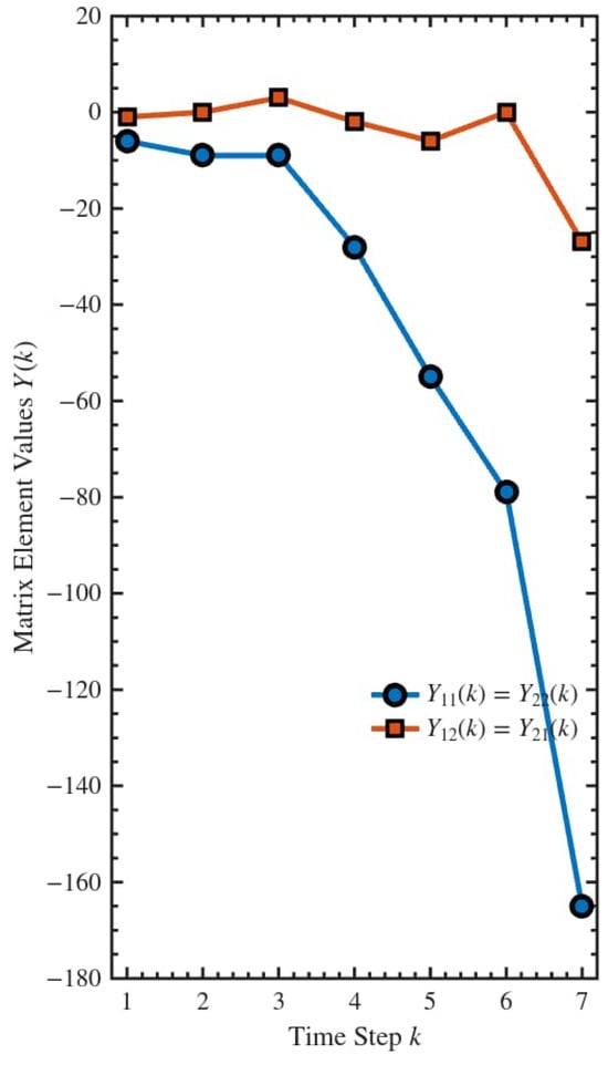
Under the initial conditions, the solution $\mathbb{Y}\left(k\right)=\left(\begin{array}{cc}{Y}_{11}\left(k\right)& Y_{12}\left(k\right)\\ Y_{21}\left(k\right)& Y_{22}\left(k\right)\end{array}\right)$ is graphed in Figure 1, and its corresponding values are listed in

Table 1. The matrix solution $\mathbb{Y}\left(k\right)$, as shown in Figure 1.

k	$\mathbb{Y}\left(\mathit{k}\right)$
1	$\left(\begin{array}{cc}-6& -1\\ -1& -6\end{array}\right)$
2	$\left(\begin{array}{cc}-9& 0\\ 0& -9\end{array}\right)$
3	$\left(\begin{array}{cc}-9& 3\\ 3& -9\end{array}\right)$
4	$\left(\begin{array}{cc}-28& -2\\ -2& -28\end{array}\right)$
5	$\left(\begin{array}{cc}-55& -6\\ -6& -55\end{array}\right)$
6	$\left(\begin{array}{cc}-179& 0\\ 0& -79\end{array}\right)$
7	$\left(\begin{array}{cc}-165& -27\\ -27& -165\end{array}\right)$

. Together, Figure 1 and Table 1 provide complementary perspectives on the behavior of the solution: the figure provides an intuitive visual understanding of the dynamic patterns, while the table provides precise numerical validation. This dual representation comprehensively demonstrates that our proposed multi-delayed discrete-matrix-exponential function successfully captures the essential dynamics of the system. Additionally, from (19), we recover the initial condition $\mathbb{Y}\left(k\right)=\Phi \left(k\right)$ for $k\in {\mathbb{Z}}_{-2}^0$. All computations and visualizations were performed using MATLAB R2023a with double precision arithmetic. The validity of our theoretical results was verified by direct substitution of the calculated solution $\mathbb{Y}\left(k\right)$ into the original Equation (17) for each $k\in {\mathbb{Z}}_1^7$. The perfect agreement between the graphical trends and numerical values confirms the robustness and accuracy of our solution methodology.

5. Conclusions

This paper resolves a significant open problem by generalizing delayed discrete-matrix equations with first-order differences from single to multiple delays. Central to this work is the introduction of a novel multi-delayed discrete-matrix exponential, ${\mathcal{E}}^{\mathbf{S},\mathbf{T}}\left(k\right)$, which extends existing delayed matrix functions. This function proved to be essential for constructing solutions to the considered class of equations. Under specific commutativity conditions, we derived an explicit solution to the initial value problem (2) in Theorem 1, generalizing several important prior results as special cases. The theoretical findings were validated by means of a numerical example, in which the explicit solution was computed and visualized.

The proposed multi-delayed matrix function establishes a foundation for future research, opening new avenues in stability analysis, controllability, and iterative learning control for multi-delayed discrete systems. Furthermore, the methodology is readily extendable to systems with non-commutative matrices, time-varying coefficients, or fractional-order differences, promising to significantly advance the theory of discrete dynamical systems with memory. For systems with non-permutable matrices, the primary challenge lies in the loss of commutative properties that enable our explicit solution’s representation. Future research could explore Baker–Campbell–Hausdorff-type formulas or develop numerical approximation schemes to handle the non-commutative case. The expected contribution would be a unified framework applicable to broader classes of practical systems where matrix commutativity cannot be assumed. Regarding time-varying coefficients, the main difficulty arises from the absence of a semigroup structure. Potential methodologies may include developing a Peano–Baker series representation or employing Magnus expansion techniques adapted for discrete delayed systems. Success in this direction would significantly enhance the model’s applicability to adaptive control and other time-dependent processes. For fractional-order differences, the challenge stems from the non-local nature of fractional operators and their complex interaction with multiple delays. Research could leverage discrete Laplace transforms or develop novel Grünwald–Letnikov-based matrix functions. This extension would bridge our work with fractional calculus, offering new tools for modeling anomalous diffusion and complex memory phenomena. Pursuing these research pathways will not only address fundamental theoretical challenges but also substantially broaden the practical impact of multi-delayed discrete systems across scientific and engineering disciplines. The explicit solution framework established in this work provides a solid foundation for these future investigations.

References

- Chen, Y. Representation of solutions and finite-time stability for fractional delay oscillation difference equations. Math. Methods Appl. Sci. 2024, 47, 3997–4013. [Google Scholar] [CrossRef]
- Huang, L.-L.; Wu, G.-C.; Luo, C. Finite-time stability of discrete fractional uncertain recurrent neural networks. Nonlinear Anal. Model. Control 2025, 30, 838–849. [Google Scholar] [CrossRef]
- Stević, S. Global stability of a max-type difference equation. Appl. Math. Comput. 2010, 216, 354–356. [Google Scholar] [CrossRef]
- Chen, Y.; Wen, C. Iterative Learning Control: Convergence, Robustness and Applications; Springer: London, UK, 1999. [Google Scholar]
- Wang, J.; Chen, D. Relative controllability of linear quaternion discrete system with delay. IEEE Trans. Automat. Control 2025, 1–8. [Google Scholar] [CrossRef]
- Yang, M.; Fečkan, M.; Wang, J. Ulam’s type stability of delayed discrete system with second-order differences. Qual. Theory Dyn. Syst. 2024, 23, 11. [Google Scholar] [CrossRef]
- Diblík, J. Relative and trajectory controllability of linear discrete systems with constant coefficients and a single delay. IEEE Trans. Autom. Control 2019, 64, 2158–2165. [Google Scholar] [CrossRef]
- Pospíšil, M. Relative controllability of delayed difference equations to multiple consecutive states. AIP Conf. Proc. 2017, 1863, 480002. [Google Scholar] [CrossRef]
- Elaydi, S.N.; Cushing, J.M. Discrete Mathematical Models in Population Biology: Ecological, Epidemic, and Evolutionary Dynamics; Springer Nature: Cham, Switzerland, 2025. [Google Scholar]
- Williamson, D. Discrete-Time Signal Processing: An Algebraic Approach; Springer: New York, NY, USA, 2012. [Google Scholar]
- Li, W.; Ren, R.; Shi, M.; Lin, B.; Qin, K. Seeking secure adaptive distributed discrete-time observer for networked agent systems under external cyber attacks. IEEE Trans. Consum. Electron. 2025; in press. [Google Scholar]
- Diblík, J. Representation of solutions to a linear matrix discrete equation with single delay. Appl. Math. Lett. 2025, 168, 109577. [Google Scholar] [CrossRef]
- Diblík, J.; Khusainov, D.Y. Representation of solutions of discrete delayed system x(k + 1) = Ax(k) + Bx(k − ϰ) + f(k) with commutative matrices. J. Math. Anal. Appl. 2006, 318, 63–76. [Google Scholar] [CrossRef]
- Diblík, J.; Khusainov, D.Y. Representation of solutions of linear discrete systems with constant coefficients and pure delay. Adv. Differ. Equ. 2006, 2006, 080825. [Google Scholar] [CrossRef]
- Diblík, J.; Morávková, B. Discrete matrix delayed exponential for two delays and its property. Adv. Differ. Equ. 2013, 2013, 139. [Google Scholar] [CrossRef]
- Diblík, J.; Morávková, B. Representation of the solutions of linear discrete systems with constant coefficients and two delays. Abstr. Appl. Anal. 2014, 2014, 320476. [Google Scholar] [CrossRef]
- Medved’, M.; Pospisil, M. Representation and stability of solutions of systems of difference equations with multiple delays and linear parts defined by pairwise permutable matrices. Commun. Appl. Anal. 2013, 17, 21–45. [Google Scholar]
- Pospisil, M. Representation of solutions of delayed difference equations with linear parts given by pairwise permutable matrices via Z-transform. Appl. Math. Comput. 2017, 294, 180–194. [Google Scholar]
- Jin, X.; Wang, J. Iterative learning control for linear discrete delayed systems with non-permutable matrices. Bull. Iran. Math. Soc. 2022, 48, 1553–1574. [Google Scholar] [CrossRef]
- Mahmudov, N.I. Delayed linear difference equations: The method of Z-transform. Electron. J. Qual. Theory Differ. Equ. 2020, 2020, 53. [Google Scholar] [CrossRef]
- Mahmudov, N.I. Multiple delayed linear difference equations with non-permutable matrix coefficients: The method of Z-transform. Montes Taurus J. Pure Appl. Math. 2024, 6, 138–146. [Google Scholar]
- Diblík, J. Representation of solutions of linear discrete systems with constant coefficients and with delays. Opuscula Math. 2025, 45, 145–177. [Google Scholar] [CrossRef]
- Medved’, M.; Škripková, L. Sufficient conditions for the exponential stability of delay difference equations with linear parts defined by permutable matrices. Electron. J. Qual. Theory Differ. Equ. 2012, 2012, 1–13. [Google Scholar] [CrossRef]
- Du, F.; Lu, J.-G. Exploring a new discrete delayed Mittag-Leffler matrix function to investigate finite-time stability of Riemann-Liouville fractional-order delay difference systems. Math. Methods Appl. Sci. 2022, 45, 9856–9878. [Google Scholar] [CrossRef]
- Liang, C.; Wang, J.; Shen, D. Iterative learning control for linear discrete delay systems via discrete matrix delayed exponential function approach. J. Differ. Equ. Appl. 2018, 24, 1756–1776. [Google Scholar] [CrossRef]
- Luo, H.; Wang, J.; Shen, D. Learning ability analysis for linear discrete delay systems with iteration-varying trial length. Chaos Solitons Fractals 2023, 171, 113428. [Google Scholar] [CrossRef]
- Jin, X.; Fečkan, M.; Wang, J. Relative Controllability of Impulsive Linear Discrete Delay Systems. Qual. Theory Dyn. Syst. 2023, 22, 133. [Google Scholar] [CrossRef]
- Agarwal, R.P. Difference Equations and Inequalities: Theory, Methods, and Applications, 2nd ed.; Marcel Dekker: New York, NY, USA, 2000. [Google Scholar]
Disclaimer/Publisher’s Note: The statements, opinions and data contained in all publications are solely those of the individual author(s) and contributor(s) and not of MDPI and/or the editor(s). MDPI and/or the editor(s) disclaim responsibility for any injury to people or property resulting from any ideas, methods, instructions or products referred to in the content. |
© 2025 by the authors. Licensee MDPI, Basel, Switzerland. This article is an open access article distributed under the terms and conditions of the Creative Commons Attribution (CC BY) license (https://creativecommons.org/licenses/by/4.0/).