Abstract
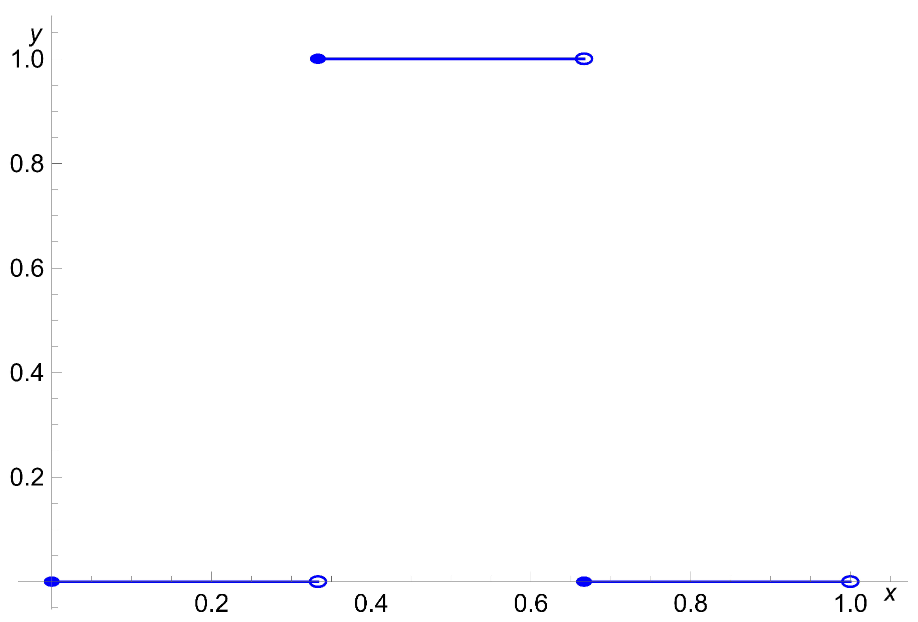
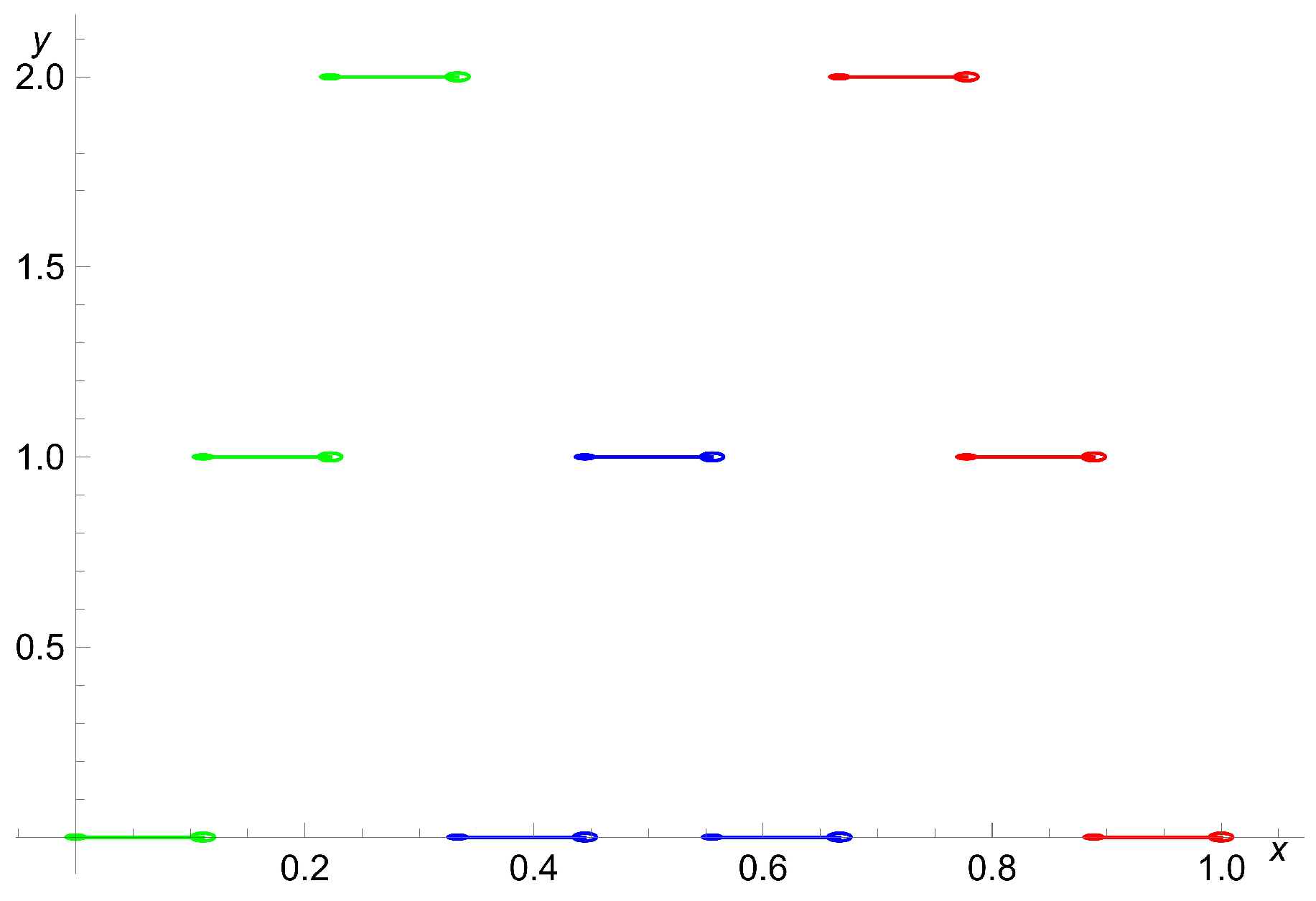
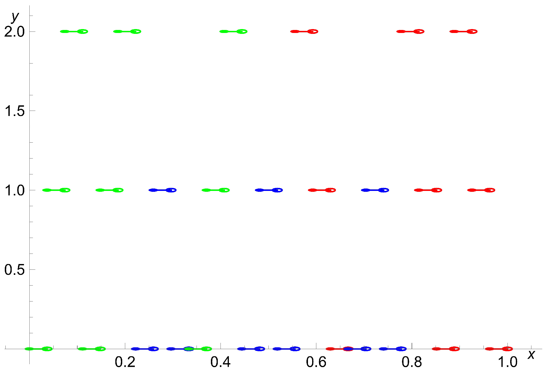
We continue the studies of derivatives of the non-harmonic series . We consider replacing with some step function . The purpose of this paper is to show that is continuous and nowhere differentiable in . All functions , used to construct f, are created from symmetrical blocks of type M: [0,1,0] and blocks of type L: [0,1,2] and R: [2,1,0], located symmetrically with respect to M. The function takes the value zero in the intervals [0,1/3), [2/3,1) and the value one in the interval [1/3,2/3), i.e., it consists of the block of type M: [0,1,0]. Function takes the value two in the intervals [2/9,3/9) and [6/9,7/9); the value one in the intervals [1/9,2/9), [4/9,5/9), and [7/9,8/9); and the value zero in the remaining intervals. This means a composition of blocks of [0,1,2][0,1,0][2,1,0], i.e., LMR blocks. The function is a symmetric composition of blocks, LLMLMRMRR. These blocks are discontinuous analogs of the functions that produces Schoenberg curves.
MSC:
Primary 26A27
1. Introduction
Chaundy and Jolliffe [1] proved the following:
Theorem 1.
If is decreasing to zero, then converges uniformly in x if and only if as .
Theorem 1 has had numerous generalizations. A result due to Žak and Šneider [2] holds for double sine series:
Theorem 2.
If is a monotonically decreasing double sequence, i.e., a sequence of real numbers such that for :
, and ,
then is uniformly regularly convergent in if and only if as .
Theorem 2 was generalized by Kórus [3]. He has defined new classes of double sequences () to obtain those generalizations.
Dyachenko, Mukanov, and Tikhonov [4] proved the Chaundy–Jolliffe theorem for sequences with majorants having the form , where is admissible.
A series
was motivation for the generalization of Theorem 1. Such series were studied by Paley and Wiener, who called them non-harmonic Fourier series. They proved that [5]:
Theorem 3.
If for , then the sequence is closed in and possesses a unique biorthogonal set , such that the series
converges uniformly to zero over interval for any positive δ, and over any such interval, the summability properties of
are uniformly the same as those of the Fourier series of .
One of the results of paper [6] is that for any converges uniformly if and only if .
In paper [7], it was proved that converges uniformly on if and only if . In paper [8], the following theorem was proved:
Theorem 4.
Let such that . If is nonincreasing and , then the series:
can be differentiated term-by-term on . The series
converges uniformly on .
In the recent paper [9], it was proved, among others, that if is a nonincreasing sequence and is convergent at any point , then .
Constructions of continuous but nowhere differentiable functions have been widely explored in the literature, particularly through the concept of fractal functions and iterated function systems. In the paper [10], some continuous interpolation functions were introduced, where I is a real closed interval, which appear ideally suited for the approximation of naturally occurring functions that display some kind of geometrical self-similarity under magnification. The new interpolation functions were referred to as fractal because they can occur such that they are not differentiable.
The paper [11] is devoted to an example of space-filling curves: Schoenberg’s curve. Sagan showed that the proof that Schoenberg’s curve is nowhere differentiable is straightforward and does not utilize any advanced notions and techniques. To produce Schoenberg’s curve, let and let be defined by: , , where is the even continuous function of period 2, which is defined in the interval (0, 1) as follows: for , for , and is linear in . It was proved that the functions are nowhere differentiable by the following lemma: If is differentiable at , then, for any two sequences , with , by necessity, exists.
We will consider a function analogous to p, which is the step function , and we will replace in a sine series considered by Chaundy and Jolliffe. will be defined by assigning values 0, 1, 2 to intervals for We will show that is continuous and nowhere differentiable on . We will be choosing a small directly so that is sufficiently large.
The book [12] is a comprehensive, self-contained compendium of results on continuous nowhere differentiable functions.
2. Main Results
Let be the sequence of functions , defined as follows:
Observe that In view of (1), depending on the value of , the function is determined on in three different ways:
First:
Therefore,
Second:
Therefore,
Third:
Therefore,
Let . Let us define:
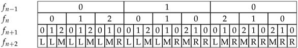
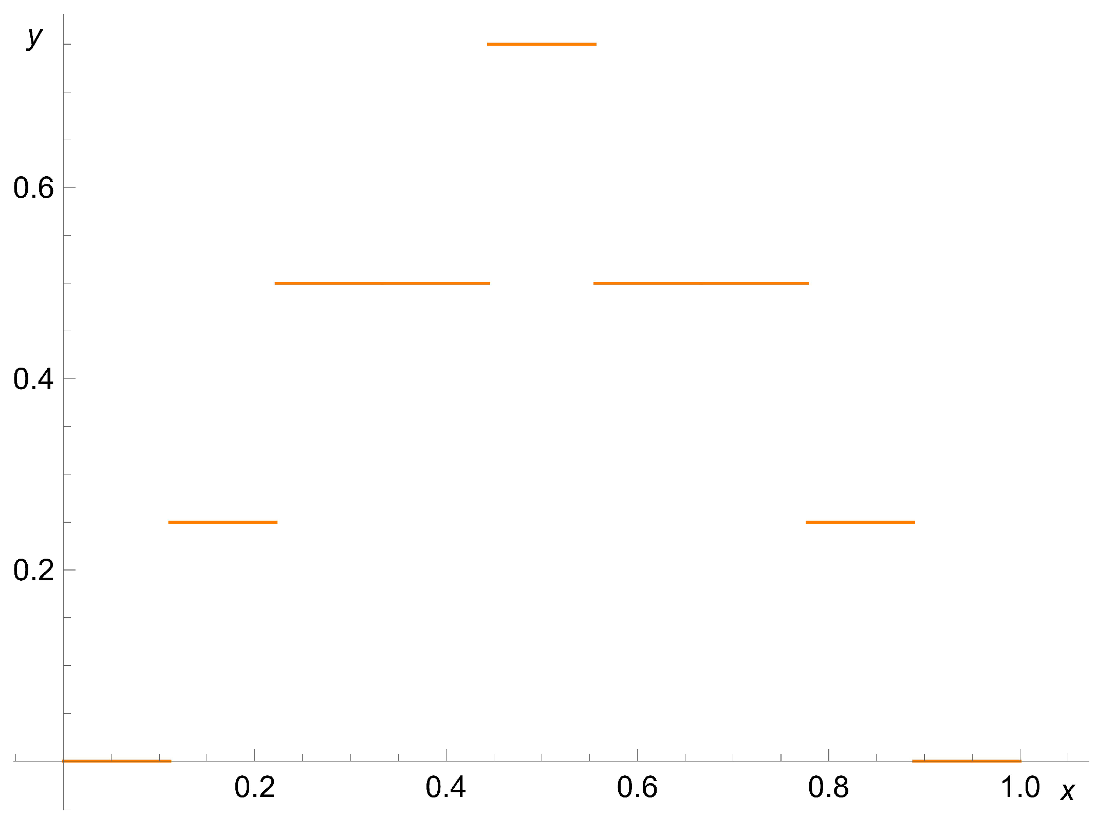
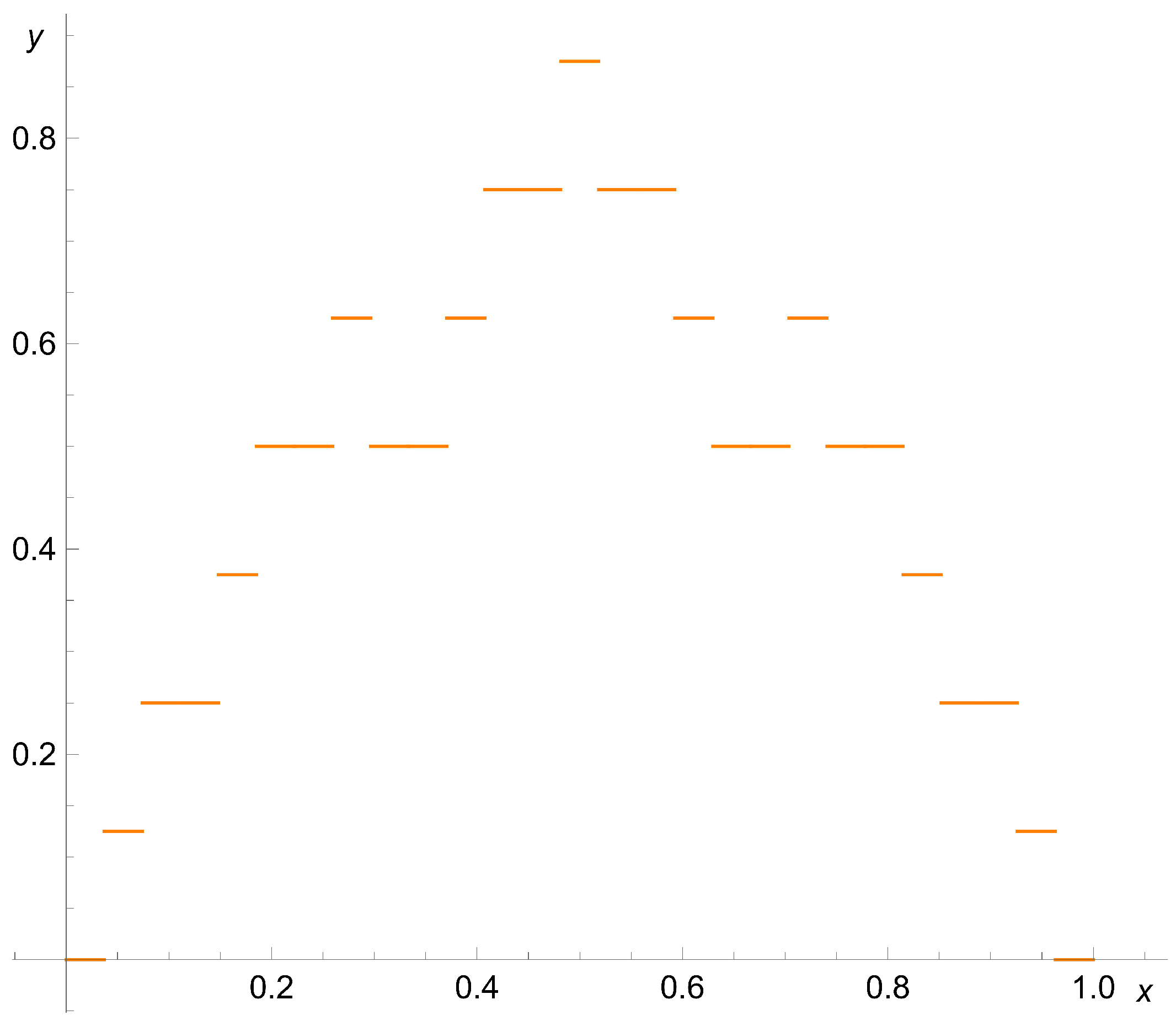
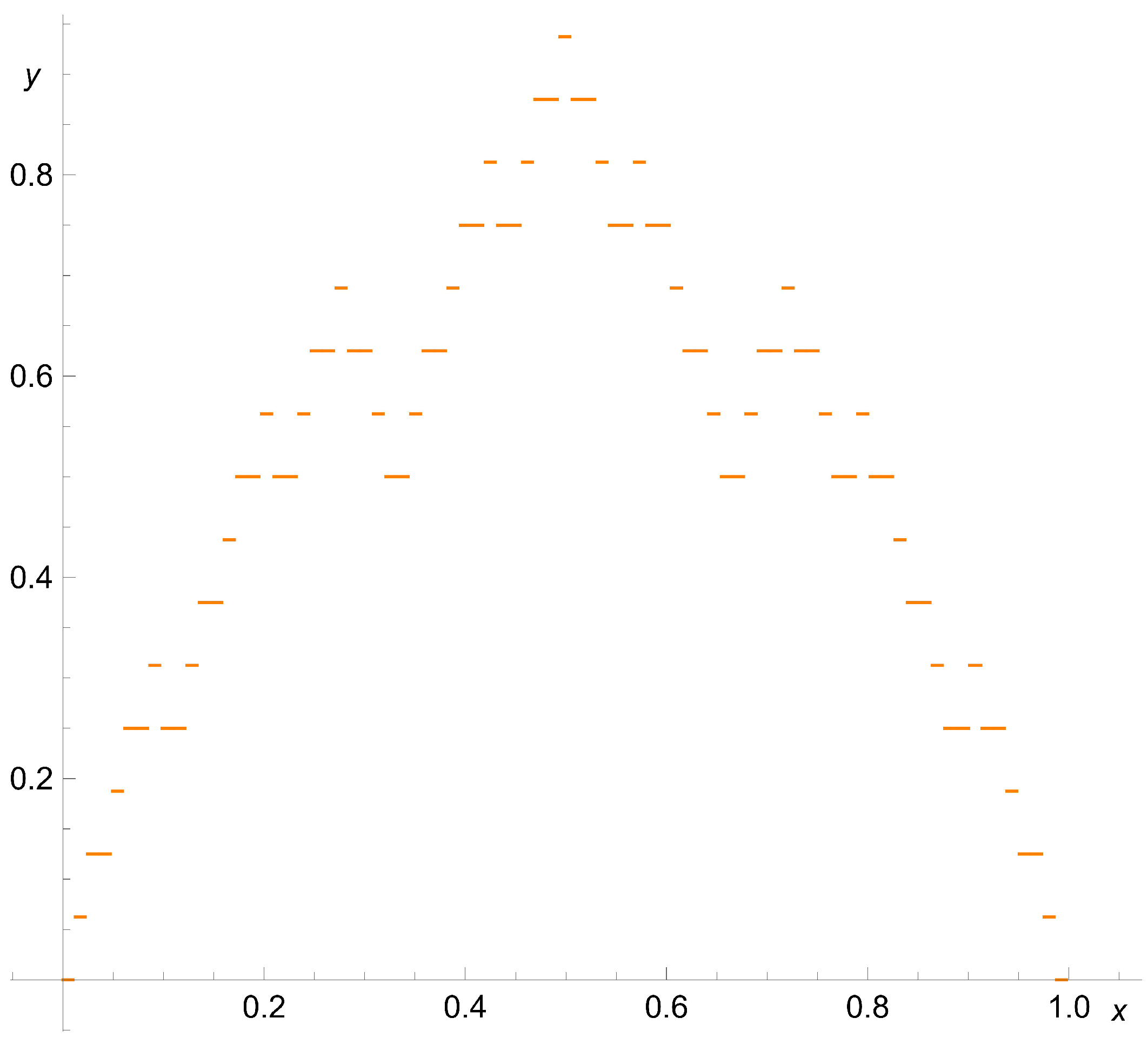
Figure 1, Figure 2 and Figure 3 show graphs of the functions Colors indicate green for L-type functions, blue for M-type functions, and red for R-type functions.
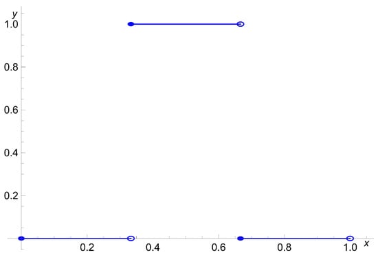
Figure 1.
The function .
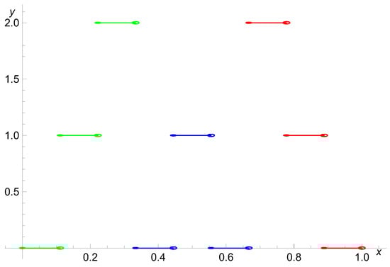
Figure 2.
The function .
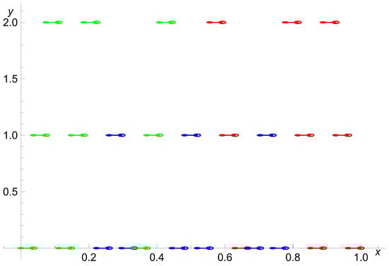
Figure 3.
The function .
Definition 5.
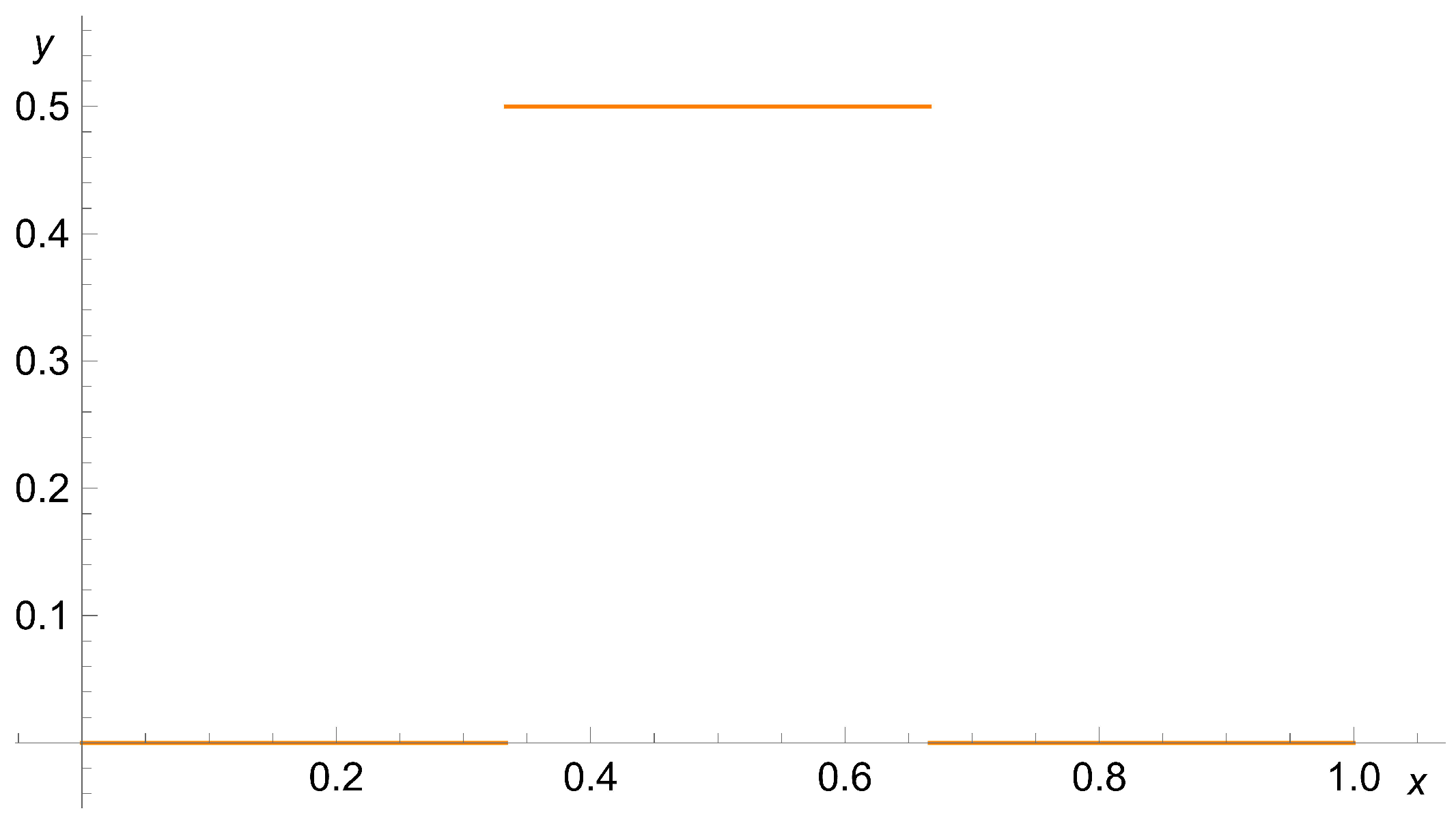
We define the function as:
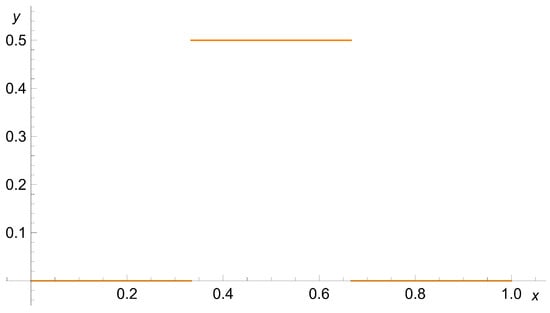
Figure 4.
The function (15) for w = 1.
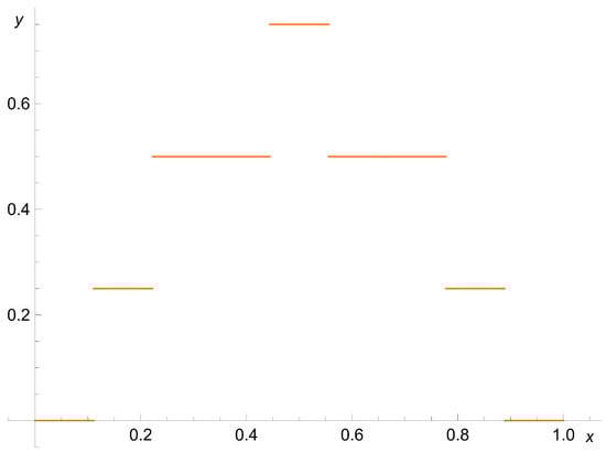
Figure 5.
The function (15) for w = 2.
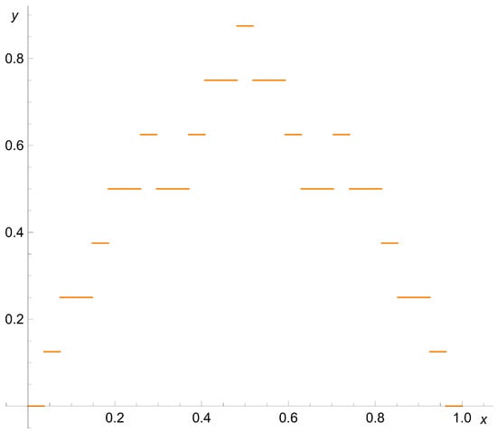
Figure 6.
The function (15) for w = 3.
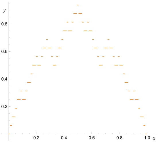
Figure 7.
The function (15) for w = 4.
Theorem 6.
The function (14) is continuous and nowhere differentiable on .
3. Proof
3.1. Continuity of the Function (14)
The series (14) is uniformly convergent. This follows from the Weierstrass M-test. Let us define , Observe that is continuous at . After considering that the series (14) is uniformly convergent, the function f is continuous at .
We consider . Observe that and .
We consider . In view of (1), the functions are continuous at ; therefore:
Moreover, . After considering that the series (14) is uniformly convergent, we obtain:
In view of (1): .
If then .
If then . Therefore:
For cases and , the proof of continuity is similar.
3.2. Non-Differentiability of the Function (14)—Scheme of Proof
Let be fixed. We will look for
so that
in the following way.
In view of (1), the function is defined by either: or or . For the sake of focus, let us assume that .
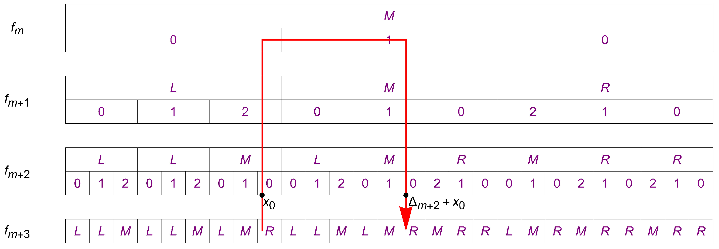
2. We choose so that: for . The way of selection is shown in the Figure 8.

Figure 8.
The way of selection .
After considering , we obtain:
and , , ,…. In the next section, we will determine precisely so that:
. For example, in Figure 8, and .
3.3. Non-Differentiability of the Function (14)—Detailed Proof
Let be a fixed real number. Then:
. Let us define .
Let us assume that the function is determined on according to (2), so that:
Case 1: .
Then, In view of (22):
Note that and
In view of (21):
Note that and
In view of (19):
In view of (20):
Case 2: .
Then, Therefore:
Case 3: .
Then, Therefore:
Case 4: .
Then, Therefore:
Case 5: .
Then, Therefore:
Case 6: .
Then, Therefore:
Case 7: .
Then, Therefore:
Case 8: .
Then, Therefore:
Case 9: .
Then, Therefore:
Case 10: .
Then, Therefore:
Case 11: .
Then, Therefore:
Case 12: .
Then, Therefore:
Case 13: .
Then, Therefore:
Case 14: .
Then, Therefore:
Case 15: .
Then, Therefore:
Case 16: .
Then, Therefore:
Case 17: .
Then, Therefore:
Case 18: .
Then, Therefore:
Case 19: .
Then, Therefore:
Case 20: .
Then, Therefore:
Case 21: .
Then, Therefore:
Case 22: .
Then, Therefore:
Case 23: .
Then, Therefore:
Case 24: .
Then, Therefore:
Case 25: .
Then, Therefore:
Case 26: .
Then, Therefore:
Case 27: .
Then, Therefore:
Let us assume that the function is determined on according to (4), so that:
Case .
Case .
Then, and we obtain:
Case .
Then , and we obtain:
Case .
Then, , and we obtain:
Case .
Then, , and we obtain:
Case .
Then, , and we obtain:
Case .
Then, , and we obtain:
Case .
Then, Therefore:
Case .
Then, Therefore:
Case .
Then, Therefore:
Case .
Then, Therefore:
Let us assume that the function is determined on according to (6), so that:
Then, , but . The proof of the theorem is finished.
4. Conclusions
This paper introduces the construction of continuous and nowhere differentiable functions using step functions. These functions are simple combinations of the three blocks [0,1,0], [0,1,2], and [2,1,0]. This allows us to directly find sufficiently small to obtain sufficiently large values of . This effect can be used in a future paper to construct continuous and nowhere differentiable functions as an infinite series of continuous and nowhere differentiable functions.
Funding
This research received no external funding.
Institutional Review Board Statement
Not applicable.
Informed Consent Statement
Not applicable.
Data Availability Statement
The original contributions presented in this study are included in the article. Further inquiries can be directed to the corresponding author.
Conflicts of Interest
The author declares no conflict of interest.
References
- Chaundy, T.W.; Jolliffe, A.E. The uniform convergence of a certain class of trigonometric series. Proc. Lond. Math. Soc. 1916, 15, 214–216. [Google Scholar]
- Žak, I.E.; Šneider, A.A. Conditions for uniform convergence of double sine series. Izv. Vysš. Učebn. Zaved. Mat. 1996, 4, 44–52. (In Russian) [Google Scholar]
- Kórus, P. On the uniform convergence of double sine series with generalized monotone coefficients. Period. Math. Hungar. 2011, 63, 205–214. [Google Scholar] [CrossRef]
- Dyachenko, M.; Mukanov, A.; Tikhonov, S. Uniform convergence of trigonometric series with general monotone coefficients. Canad. J. Math. 2019, 71, 1445–1463. [Google Scholar] [CrossRef]
- Levinson, N. Gap and Density Theorems; AMS Colloquium Publications: New York, NY, USA, 1940; Volume 26. [Google Scholar]
- Oganesyan, K.A. Uniform convergence criterion for non-harmonic sine series. Sb. Math. 2021, 212, 70. [Google Scholar] [CrossRef]
- Kęska, S. On the uniform convergence of sine series with square root. J. Funct. Spaces 2019, 2009, 1342189. [Google Scholar] [CrossRef]
- Kęska, S. A Note on Derivative of Sine Series with Square Root. Abstr. Appl. Anal. 2021, 2021, 7035776. [Google Scholar] [CrossRef]
- Gabdullin, M. Trigonometric series with noninteger harmonics. J. Math. Anal. Appl. 2022, 508, 125792. [Google Scholar] [CrossRef]
- Barnsley, M.F. Fractal functions and interpolation. Constr. Approx. 1986, 2, 303–329. [Google Scholar] [CrossRef]
- Sagan, H. An elementary proof that Schoenberg’s space-filling curve is nowhere differentiable. Math. Mag. 1992, 65, 125–128. [Google Scholar] [CrossRef]
- Jarnicki, M.; Pflug, P. Continuous Nowhere Differentiable Functions, the Monster of Analysis; Springer: Berlin/Heidelberg, Germany, 2015. [Google Scholar]
Disclaimer/Publisher’s Note: The statements, opinions and data contained in all publications are solely those of the individual author(s) and contributor(s) and not of MDPI and/or the editor(s). MDPI and/or the editor(s) disclaim responsibility for any injury to people or property resulting from any ideas, methods, instructions or products referred to in the content. |
© 2025 by the author. Licensee MDPI, Basel, Switzerland. This article is an open access article distributed under the terms and conditions of the Creative Commons Attribution (CC BY) license (https://creativecommons.org/licenses/by/4.0/).