An Optimal Investment Decision Problem Under the HARA Utility Framework

Abstract

This paper is dedicated to studying the optimal investment proportions of three types of assets with symmetry, namely, risky assets, risk-free assets, and wealth management products, when the stochastic expenditure process follows a jump-diffusion model. The stochastic expenditure process is treated as an exogenous cash flow and is assumed to follow a stochastic differential process with jumps. Under the Cox–Ingersoll–Ross interest rate term structure, it is presumed that the prices of multiple risky assets evolve according to a multi-dimensional geometric Brownian motion. By employing stochastic control theory, the Hamilton–Jacobi–Bellman (HJB) equation for the household portfolio problem is formulated. Considering various risk-preference functions, particularly the Hyperbolic Absolute Risk Aversion (HARA) function, and given the algebraic form of the objective function through the terminal-value maximization condition, an explicit solution for the optimal investment strategy is derived. The findings indicate that when household investment behavior is characterized by random expenditures and symmetry, as the risk-free interest rate rises, the optimal proportion of investment in wealth-management products also increases, whereas the proportion of investment in risky assets continually declines. As the expected future expenditure increases, households will decrease their acquisition of risky assets, and the proportion of risky-asset purchases is sensitive to changes in the expectation of unexpected expenditures.

1. Introduction

In the modern investment management system, asset allocation is a crucial component of the portfolio management optimization problem. How to effectively perform asset allocation in investments is a concern shared by many financial scholars. Lu Xiaomeng et al. [1] have pointed out that in order to develop a portfolio strategy to meet the expectations of investors, the risk and income control is the most important issue in the asset allocation.

In terms of the introduction of stochastic interest rates, in recent years, Liu et al. [2] found the optimal investment strategy under exponential utility and logarithmic utility function on the basis of random volatility of risk assets. Ferland and Watier [3] characterized the risk-free interest rate in the mean-variance model by using the CIR interest rate model, and obtained the explicit solution of the optimal investment strategy by using the stochastic differential equation theory. Chang Hao et al. [4] studied the individual optimal investment and consumption strategy based on the CEV model under the Vasicek interest rate model. Guan and Liang [5] introduced the stochastic interest rate and stochastic volatility model into DC pension management; Chang and Chen [6] selected the HARA utility function to study the investment problem of the pension fund in an environment of stochastic interest rates and stochastic volatility. In the portfolio optimization problem, adding random interest rate and random volatility to the description of assets will make the optimal investment strategy obtained by the model more practical.

When considering appropriate utility functions, the HARA (Hyperbolic Absolute Risk Aversion) utility function can encompass various types of risk preferences. It has a high degree of compatibility with the real-world market and is of great practical significance. In the study of asset allocation of self-financing portfolios and optimal portfolio strategies, Zhao and Rong [7] studied the multi-asset allocation model under the framework of CARA utility function. Chang et al. [8] obtained the optimal portfolio strategy under different utility functions on the portfolio allocation problem with random interest rate and random volatility. Bakkaloglu et al. [9] also studied a portfolio allocation problem based on stochastic interest rates and stochastic volatility. Rong and Fan [10] applied the utility function framework of CRRA and CARA to the optimal investment problem of insurers, and obtained the explicit solution of the optimal strategy under different utility functions in insurance investment. Gu et al. [11] obtained the optimal investment strategy under the framework of CARA and CRRA utility function by proportional optimal reinsurance. Li et al. [12] obtained a more comprehensive and realistic optimal investment strategy considering the portfolio optimization problem under various expected utility functions. Lin and Li [13] regard the entire insurance company’s earnings process as a jump-diffusion process, and obtained the explicit solution of the optimal strategy under the framework of CARA utility function.

In the general dynamic portfolio problem under the framework of time-additive expected utility, scholars have explored the direction of more generalized investor utility. Huang and Milevsky [14] studied the dynamic asset portfolio problem of claims in unexpected situations under the HARA utility framework. Jung and Kim [15] joined the concept of default risk to study the problem of investment and consumption under the HARA utility function. Bo et al. [16] studied the investment consumption problem with default risk under the HARA utility function, and analyzed the specific investment strategies under different parameters. Chang et al. [17] gave an optimal strategy for asset–liability problems with an affine interest rate under the framework of HARA utility. Nie [18] studied the reality of the optimal investment strategy to transfer the claim risk by purchasing proportional reinsurance combined with the CEV process and maximizing the HARA utility. Zhang ang Wang [19] utilized the Legendre dual transformation to study the optimal investment-reinsurance problem of maximizing the Hyperbolic Absolute Risk Aversion (HARA) utility under the Ornstein-Uhlenbeck (O-U) risk model.

We are dedicated to studying the optimal allocation of household assets across risky assets, risk-free assets, and financial products, with the aim of determining the most realistic optimal investment proportions for household assets. Ultimately, by explicitly expressing these optimal proportions, we analyze the dynamic impact mechanisms of various parameters on the strategy, thereby providing a more intuitive theoretical basis for household investment activities.

In the context of household portfolio problems, not only investment risks but also the risks brought about by unexpected expenditures need to be considered. Yuan and Lai [20] hold that household expenditures include consumption expenditures, and such expenditures are also a type of stochastic cash flow. They added stochastic expenditures to the original self-financing portfolio. Consequently, they incorporated stochastic expenditures into the original self-financing portfolio framework. The innovations of this study are as follows: (1) Assuming that the prices of multiple risky assets follow geometric Brownian motion, and taking into account stochastic interest rates and a jump-diffusion-based stochastic expenditure process, this study investigates the optimal asset allocation problem by incorporating the stochastic price process of financial products, which is influenced by the fluctuations of stochastic interest rates. Therefore, this paper extends the work of [6,20]. (2) For the symmetrical allocation of risky assets, risk-free assets, and wealth management products, more realistic optimal investment proportions of family assets are obtained through the application of initial value and terminal value problems [21]. Finally, the explicit expressions of the optimal proportions are used to analyze the dynamic influence mechanism of various parameters on the strategy, so as to provide a more intuitive theoretical basis for family investment activities.

2. Research Methods

We utilize a jump-diffusion model to simulate the dynamics of asset prices. Stochastic control theory is applied to derive the optimal investment strategy.

Firstly, considering the fundamental assumptions, the asset allocation model in continuous time is established in this section. Given a Markov economy defined in $\left[0,T\right]$ continuous time, all uncertainties in the investment period are defined by a complete probability space $\left(\Omega ,F,{\left\{F_t\right\}}_{0\le t\le T},{\rm P}\right)$, where P is a risk neutral probability and $F=\left\{F_t\right\}$ is a right continuous $\sigma$—algebraic space, which represents all available information sets before all t moments. The random process in this paper is applicable to this information basin, and the following hypothesis is given:

(1)

It is assumed that the asset can be split infinitely and can be continuously traded within [0, T];

(2)

It is assumed that there are no transaction costs and tax costs in the financial market;

(3)

Since the article mainly analyzes the influence of random expenditures, the randomness of wage income is not considered for the time being.

It is assumed that the financial market is composed of three types of symmetrical assets, that is, one risk-free asset, multiple risky assets, and one wealth management product. And it is assumed that the financial market is complete and continuously tradable. Given the complexity of the actual investment environment, it is assumed that during an investment cycle, multiple random factors simultaneously affect households. Therefore, during the investment period, the risk-free asset price $S_0\left(t\right)$ at time t satisfies the following stochastic process:

$$d{S}_0\left(t\right)=r\left(t\right)S_0\left(t\right)dt,\begin{array}{cc}& S_0\left(0\right)=1\end{array}$$

(1)

The initial price of the risk-free asset is 1, and $r\left(t\right)$ represents the risk-free interest rate, which follows a stochastic process that models the term structure of interest rates. The Cox–Ingersoll–Ross (CIR) model, proposed by John Cox, Jonathan Ingersoll, and Stephen Ross in 1985, is a mathematical model used to describe the dynamics of interest rates. Since interest rates in a continuous financial investment environment always fluctuate around an average value, the CIR interest rate model is employed here to characterize the risk-free interest rate. The risk-free interest rate at time t is given as follows:

$$dr\left(t\right)=\left(a-br\left(t\right)\right)dt-k\sqrt{r\left(t\right)}d{W}_r\left(t\right),\begin{array}{cc}& r\left(0\right)=r_0\end{array}>0$$

(2)

where a, b, k is the constant greater than 0, 1/b is the mean reversion speed, k is the volatility parameter, and $W_r\left(t\right)$ is the standard Brownian motion defined in the complete probability space $\left(\Omega ,F,P\right)$ in one dimension.

The limitations of the CIR model assumptions include that interest rates are always non-negative and revert linearly to a long-term mean, which may not fully capture real-world scenarios. However, by understanding the practical significance of these parameters and the model’s limitations, the CIR model can be better applied for interest rate analysis and forecasting.

Considering that in real-world investment environments households often choose to invest in more than one type of risky asset, among the risky assets with symmetry, assume that the price of the i-th risky asset at a certain moment during the investment period is $S_i\left(t\right),i=1,2,3,\cdots ,n$, which follows the following stochastic process [22]:

$${\displaystyle \frac{d{S}_i\left(t\right)}{S_i\left(t\right)}}=r\left(t\right)dt+{\displaystyle \sum _{j=1}^n{\sigma }_{ij}\left(d{W}_j\left(t\right)+{\lambda }_{j}dt\right)+{\sigma }_{ir}\sqrt{r\left(t\right)}\left(d{W}_r\left(t\right)+{\lambda }_r\sqrt{r\left(t\right)}dt\right)}$$

(3)

$$S_i\left(0\right)=s_i>0$$

Among them, ${\lambda }_s={\left({\lambda }_1,\cdots ,{\lambda }_j,\cdots ,{\lambda }_n\right)}^{\prime }$ represents the influence coefficient of the price change of risky assets on the return of risky assets. Since a variety of risks exist at the same time and act together, ${\sigma }_s={\left({\sigma }_{ij}\right)}_{n\times n}$ is the volatility matrix generated by the price changes of risky assets. Then, ${\sigma }_r={\left({\sigma }_{1r},{\sigma }_{2r},\cdots ,{\sigma }_{nr}\right)}^{\prime }$ denotes the volatility matrix caused by random interest rate changes, ${\lambda }_r$ denotes the influence coefficient of random interest rate fluctuations on the return of risk assets. $W_s\left(t\right)=\left(W_1\left(t\right),W_2\left(t\right),\cdots ,W_n\left(t\right)\right)$ denotes the n-dimensional independent Brownian motion defined in the complete probability space $\left(\Omega ,F,P\right)$, and $W_s$ and $W_r$ are independent of each other. $s_i\left(0\right)$ denotes the initial price of the i-th risk asset during the investment period.

The other symmetry asset is financial products. After the 19th National Congress of the Communist Party of China, the investment behavior of families in real estate has been reduced, and the participation rate of stocks and equity funds has increased. Therefore, in the traditional model setting link, the key financial assets which are consistent with the actual assets should be added to the decision-making problem of the family investment portfolio, such as the random process of financial products such as funds between risk assets and risk-free assets, so that the optimal strategy of family investment portfolios is more practical.

Assuming that the duration of financial products is $T$, the price at time $t$ during the investment period is denoted as $B\left(t\right)$. Affected by the random interest rate, it becomes a special risk asset that changes with the interest rate. The price change process satisfies the following stochastic differential equation [22]:

$${\displaystyle \frac{dB\left(t\right)}{B\left(t\right)}}=r\left(t\right)dt+{\sigma }_B\left(d{W}_r\left(t\right)+{\lambda }_r\sqrt{r\left(t\right)}dt\right),\begin{array}{cc}& B\left(T\right)\end{array}=1$$

(4)

where ${\sigma }_B=kh\left(t\right)\sqrt{r\left(t\right)}$ is the instantaneous price volatility of financial products and is affected by random interest rates, where

$$h\left(t\right)={\displaystyle \frac{2\left(1-e^{m\left(T-t\right)}\right)}{\sqrt{{\left(b-{\lambda }_{r}k\right)}^2+2k^2}-b+{\lambda }_{r}k+e^{m\left(T-t\right)}\left(m+b-{\lambda }_{r}k\right)}}$$

(5)

And $k$ and $b$ are constants greater than 0, $m$ is the discount factor.

To ensure the smooth operation of household investment activities, it is inevitable that unexpected expenditures may arise during the entire investment period. We model these cumulative unexpected expenditures as a jump-diffusion process (due to the unpredictability of expenditures in actual investment processes, such as imbalances in unexpected insurance revenues and expenses caused by global diseases, incorporating a stochastic expenditure process can better prepare for such events, thereby achieving an optimal investment portfolio strategy). The household expenditure process E(t) at time t satisfies the following stochastic differential equation:

$${\displaystyle \frac{dE\left(t\right)}{E\left(t\right)}}={\mu }_{E}dt+{\sigma }_{E}d{M}_t+d{\displaystyle \sum _{i=1}^{N\left(t\right)}{Y}_i}\begin{array}{cc}& E_0=e_0\end{array}$$

(6)

where $M_t$ is a one-dimensional standard Brownian motion, ${\mu }_E$ is a normal number that represents the instantaneous expected expenditure of the family, ${\sigma }_E$ is a constant that represents the instantaneous volatility of household random expenditure, $N\left(t\right)$ is the number of jumps in expenditure prices, $Y_i$ represents the magnitude of the first jump in expenditure prices, and is a series of independent and identically distributed random variables. assuming that $M_t$ and ${\displaystyle \sum _{i=1}^{N\left(t\right)}{Y}_i}$ are independent, where, $N\left(t\right)$ obeys a Poisson process with degrees of freedom ${\lambda }_E$, ${\lambda }_E{b}_E$ is the expected value of random spending, $\sqrt{{\lambda }_E}{a}_E$ is the instantaneous volatility of household spending. Here, when the fixed income is $C$ and $C\le {\lambda }_E{b}_E$, the household spending risk will cause the initial endowment to reach a negative effect. At this time, there will be a risk of bankruptcy, which will not be discussed here. The subsequent analysis of default assumptions involves $C>{\lambda }_E{b}_E$. Since interest rate changes are an important means of causing household consumption, and the random fluctuations of interest rates in the investment environment have a certain impact on the unexpected expenditure of household wealth, Brownian motion $W_r$ and $M_t$ have a correlation, and the correlation coefficient is $\rho$, which is $d{W}_r\cdot d{M}_t=\rho dt$.

In the jump risk process, obtaining the optimal explicit solution for the classical compound Poisson process is challenging. Therefore, the diffusion approximation method is employed to transform the jump diffusion process (6) into a Brownian motion process:

$$dE\left(t\right)=E\left(t\right){\lambda }_E{b}_{E}dt-E\left(t\right)\sqrt{{\lambda }_E}{a}_{E}d{M}_t$$

(7)

Proof. 

The jump risk process is $E\left(t\right)=ct+{\displaystyle \sum _{i=1}^{N\left(t\right)}{Y}_i}$. At this time, take $E\left(t\right)\to {\displaystyle \frac{E\left(nt\right)}{\sqrt{n}}}$, the limit process $E^{\prime }$ can be obtained, $d{E}^{\prime }={\mu }_{e}dt+{\sigma }_{e}d{M}_t$, where ${\mu }_e=\lambda m_e\begin{array}{cc},& {{\sigma }_e}^2=\lambda \left(m_e+{s_e}^2\right),\end{array}$ $m_e\begin{array}{cc},& {s_e}^2\end{array}$ is the expectation and variance of the i-th family expenditure. Let $b_E=m_e$, ${a_E}^2=m_e+{s_e}^2$. Results (7) are certificated. □

3. Results

3.1. The Family Wealth Process

$V_t$ is the total disposable wealth of the household at the moment $t\in \left[0,T\right]$ of the investment period; household fixed income is $C$. Let the proportion of funds invested in zero-coupon bonds be ${\pi }_B\left(t\right)$, The proportion of capital invested in the i-th risky asset is ${\pi }_i\left(t\right)$, ${{\pi }_i}^{\prime }\left(t\right)={\left({\pi }_1\left(t\right),{\pi }_2\left(t\right),\cdots ,{\pi }_n\left(t\right)\right)}^{\prime }$. Then, the proportion of investment in risk-free assets is ${\pi }_0\left(t\right)=1-{\displaystyle \sum _{i=1}^n{\pi }_i\left(t\right)-{\pi }_B\left(t\right)}$. Then, the differential equation of the family wealth process is

$$d{V}_t={\pi }_0\left(t\right)V_t{\displaystyle \frac{d{S}_0\left(t\right)}{S_0\left(t\right)}}+{\displaystyle \sum _{i=1}^n{\pi }_i\left(t\right)}{V}_t{\displaystyle \frac{d{S}_i\left(t\right)}{S_i\left(t\right)}}+{\pi }_B\left(t\right)V_t{\displaystyle \frac{dB\left(t\right)}{B\left(t\right)}}+Cdt-E\left(t\right)dt$$

(8)

Putting the differential equation into the above formula, we obtain

$$\begin{gathered} d{V}_t=\left[V_t{r}_t+{\pi }_B{V}_t{\sigma }_B{\lambda }_r\sqrt{r\left(t\right)}+V_t{{\pi }_i}^{\prime }\left({\sigma }_s{\lambda }_s+{\sigma }_r{\lambda }_{r}r\left(t\right)\right)-{\lambda }_E{b}_E+C\right]dt+V_t{{\pi }_s}^{\prime }{\sigma }_{s}d{W}_s \\ +\left[V_t{{\pi }_i}^{\prime }{\sigma }_r\sqrt{r\left(t\right)}+{\pi }_B{V}_t{\sigma }_B\right]d{W}_r-a\sqrt{{\lambda }_E}d{M}_t \end{gathered}$$

(9)

3.2. HJB Equation

We will give the general form of $\underset{{\pi }_t\in \Pi }{\max }E\left\{U\left(V_T\right)\right\}$, maximize the expected utility of household wealth at the terminal moment, and give the HJB equation of $\underset{{\pi }_t\in \Pi }{\max }E\left\{U\left(V_T\right)\right\}$ according to the dynamic programming method, where $\Pi$ denotes the set of all admissible policies and $U\left(\cdot \right)$ denotes the utility function. The Hamilton–Jacobi–Bellman (HJB) equation is a core equation in dynamic programming, used to solve optimal control problems. In the context of investment strategies, it helps to determine the optimal decisions under given states (such as wealth level and market conditions). Methods for computing the HJB model mainly include the finite difference method, Monte Carlo simulation, the finite element method, and deep reinforcement learning. Compared to other methods, solving the equation analytically prior to conducting numerical simulations can reduce errors and improve the analyzability of the parameters. In the process of solving the HJB equation, the variables and parameters involved include state variables such as wealth level and interest rate; control variables such as investment proportion; parameters such as the risk aversion coefficient and market parameters; and boundary conditions such as initial wealth and the terminal utility function.

According to the classical stochastic optimal control, the value functions for time $t$, instantaneous interest rate $r$, and household wealth $v$ are defined as follows:

$$H\left(t,r,v\right)=E\left\{U\left(V_T\right)\left|r\left(t\right)=r,V_t=v\right.\right\},\begin{array}{cc}& 0\le t\le T\end{array}$$

(10)

Then, the optimal value function is

$$H\left(t,r,v\right)=\underset{{\pi }_B\in \Pi ,{\pi }_s\in \Pi }{\sup }H\left(t,r,v\right)$$

where the boundary conditions are $H\left(T,r,v\right)=U\left(V_T\right)$. According to the principle of dynamic programming, we obtain the following HJB equation as follows:

$$\begin{gathered} 0=\underset{{\pi }_B\in \Pi ,{\pi }_s\in \Pi }{\sup }\{H_t+\left(a-br\right)H_r+\left(r{v}_t+{\pi }_B{v}_t{\sigma }_B{\lambda }_r\sqrt{r}+{\pi }_s^{\prime }{v}_t\left({\sigma }_s{\lambda }_s+{\sigma }_r{\lambda }_{r}r\right)-{\lambda }_E{b}_E+C\right)H_v \\ +\frac{1}{2}\left[{\left({\pi }_s^{\prime }{v}_t{\sigma }_s\right)}^2+{\left({\pi }_s^{\prime }{v}_t{\sigma }_r\sqrt{r}+{\pi }_B{v}_t{\sigma }_B\right)}^2+a^2{\lambda }_E-\rho a_E\sqrt{{\lambda }_E}\left(v_t{\pi }_s^{\prime }{\sigma }_r\sqrt{r}+{\pi }_B{v}_t{\sigma }_B\right)\right]H_{vv} \\ +\frac{1}{2}{k}^{2}r{H}_{rr}-k\sqrt{r}\left({\pi }_s^{\prime }{v}_t{\sigma }_r\sqrt{r}+{\pi }_B{v}_t{\sigma }_B+\rho a_E\sqrt{{\lambda }_E}k\sqrt{r}\right)H_{rv}\} \end{gathered}$$

(11)

where $H_t,H_r,H_v,H_{rr},H_{rv},H_{vv}$ are the first and second partial derivatives of the value function with respect to time $t$, risk-free rate $r$, and household wealth $v$. Now, according to the first-order condition of the extreme value, the optimal strategies ${\pi }_{\mathrm{B}}^{\ast }$ (the investment ratio of financial products) and ${\pi }_s^{\ast }$(the investment ratio of risk assets) are solved:

$${{\pi }_B}^{\ast }={\displaystyle \frac{k\sqrt{r}}{v{\sigma }_B}}{\displaystyle \frac{H_{rv}}{H_{vv}}}+{\displaystyle \frac{\left({\lambda }_s^{\prime }{\sigma }_s^{-1}{\sigma }_r-{\lambda }_r\right)\sqrt{r}}{v{\sigma }_B}}{\displaystyle \frac{H_v}{H_{vv}}}+{\displaystyle \frac{\rho a_E\sqrt{{\lambda }_E}}{2v{\sigma }_B}}-{\displaystyle \frac{\rho a_E\sqrt{{\lambda }_E}{\sigma }_r^{2}r}{2v{\sigma }_B{\sigma }_s^{\prime }{\left({\sigma }_s^{\prime }\right)}^T}}$$

$${{\pi }_s}^{\ast }=-{\displaystyle \frac{{\lambda }_s}{v}}{\left({\sigma }_s^{\prime }\right)}^{-1}{\displaystyle \frac{H_v}{H_{vv}}}+{\displaystyle \frac{\rho a_E\sqrt{{\lambda }_E}{{\sigma }_r}^3{r}^{\frac{3}{2}}}{2v{\sigma }_s^{\prime }{\left({\sigma }_s^{\prime }\right)}^T\left({{\sigma }_r}^{2}r+{\sigma }_s^{\prime }{\left({\sigma }_s^{\prime }\right)}^T\right)}}$$

(12)

Substitute the above two results into the HJB equation and simplify reasonably to obtain the optimal value function:

$$\begin{gathered} 0=H_t+\left(a-br\right)H_r+\left(rv-{\lambda }_E{b}_E+C\right)H_v+\frac{1}{2}{a}^2{\lambda }_E{H}_{vv}+\frac{1}{2}{k}^{2}r{H}_{rr}-k^{2}r\rho a_E\sqrt{{\lambda }_E}{H}_{rv} \\ +\frac{3}{2}\rho a_E{\lambda }_r\sqrt{{\lambda }_{E}r}{H}_v-{\displaystyle \frac{\rho a_E\sqrt{{\lambda }_E}{r}^{\frac{3}{2}}{\sigma }_r^3{\lambda }_s}{2{\sigma }_s{\sigma }_s^{-1}{\sigma }_s}}{H}_v-\frac{1}{2}\left({‖{\lambda }_s‖}^2+{\lambda }_r^{2}r\right){\displaystyle \frac{H_v^2}{H_{vv}}}+kr{\lambda }_r{\displaystyle \frac{H_v{H}_{rv}}{H_{vv}}}-\frac{1}{2}{k}^{2}r{\displaystyle \frac{H_{rv}^2}{H_{vv}}} \\ +{\displaystyle \frac{{\rho }^2{a}_E^2{\lambda }_E\left({\sigma }_r^6{r}^3{\sigma }_s^2+2{\sigma }_r^8{r}^4-2{\sigma }_s^4{\sigma }_r^4{r}^2+8{\sigma }_r^{2}r{\sigma }_s^6-3{\sigma }_s^8\right)}{8{\sigma }_s^2{\left({\sigma }_r^{2}r+{\sigma }_s^2\right)}^2}}{H}_{vv}-{\displaystyle \frac{k\rho a_E\sqrt{{\lambda }_E}{\sigma }_r^4{r}^{\frac{5}{2}}}{2{\sigma }_s^2\left({\sigma }_r^{2}r+{\sigma }_s^2\right)}}{H}_{rv} \\ -k\rho a_E\sqrt{{\lambda }_{E}r}{H}_{rv}-{\displaystyle \frac{k\rho a_E\sqrt{{\lambda }_E}{\sigma }_r^4{r}^{\frac{5}{2}}}{2{\sigma }_s\left({\sigma }_r^{2}r+{\sigma }_s^2\right)}}{\displaystyle \frac{H_{rv}}{H_{vv}}} \end{gathered}$$

(13)

3.3. Explicit Results Under the HARA Utility Function

In this section, the household investment process is still regarded as a stochastic optimal control problem. The Hamilton–Jacobi–Bellman (HJB) equation is derived under the same value function through the principle of dynamic programming. During the process of interest rate marketization, households aim to obtain the optimal investment strategy and maximize the expected utility corresponding to wealth throughout the entire non-self-financing portfolio investment. This represents the optimal strategy achieved under the general utility function. Now, consider a family with hyperbolic absolute risk aversion (HARA) preferences, which encompasses many common utility functions, namely,

$$U\left(v\right)={\displaystyle \frac{1-x}{xy}}{\left({\displaystyle \frac{y}{1-x}}v+\gamma \right)}^x, y<0,x<1,x\ne 0$$

(14)

(1)

Power utility, when $\gamma =0,y=1-x$, $U\left(v\right)=U_{CBBA}\left(v\right)$;

(2)

Index utility, when $\gamma =1,x\to -\infty$, $U\left(v\right)=U_{CABA}\left(v\right)$;

(3)

Logarithmic utility, when $\gamma =0,x\to 0,y\to 1$, $U\left(v\right)=U_{\log }\left(v\right)$.

According to terminal conditions,

$$H\left(T,r,v\right)=U\left(v\right)$$

(15)

Lemma 1.

We consider the following form of value function:

$$H\left(t,r,v\right)={\displaystyle \frac{1-x}{xy}}{\left({\displaystyle \frac{y}{1-x}}v+\gamma \varphi \left(t,r\right)\right)}^x{f}^{1-x}\left(t,r\right)$$

(16)

And Equation (16) satisfies the terminal conditions:

$$\varphi \left(T,r\right)=1, f\left(T,r\right)=1$$

(17)

Proof. 

The explicit analytical expressions of the final value condition and the value function are given, and then the differentials of the two sides of Equation (16) with respect to $t,r,v$ are calculated. The results are as follows:

$$H_t={\displaystyle \frac{1-x}{y}}{\left({\displaystyle \frac{y}{1-x}}v+\gamma \varphi \right)}^{x-1}\gamma {\varphi }_t{f}^{1-x}+{\displaystyle \frac{{\left(1-x\right)}^2}{xy}}{\left({\displaystyle \frac{y}{1-x}}v+\gamma \varphi \right)}^x{f}_t{f}^{-x}$$

$$H_r={\displaystyle \frac{1-x}{y}}\gamma {\varphi }_r{f}^{1-x}{\left({\displaystyle \frac{y}{1-x}}v+\gamma \varphi \right)}^{x-1}+{\displaystyle \frac{{\left(1-x\right)}^2}{xy}}{f}^{-x}{f}_r{\left({\displaystyle \frac{y}{1-x}}v+\gamma \varphi \right)}^x$$

$$H_v=f^{1-x}{\left({\displaystyle \frac{y}{1-x}}v+\gamma \varphi \right)}^{x-1},\begin{array}{cc}& \end{array}{H}_{vv}=\left(-y\right)f^{1-x}{\left({\displaystyle \frac{y}{1-x}}v+\gamma \varphi \right)}^{x-2}$$

$$\begin{gathered} H_{rr}={\displaystyle \frac{{\left(1-x\right)}^2}{-y}}{\gamma }^2{{\varphi }_r}^2{f}^{1-x}{\left({\displaystyle \frac{y}{1-x}}v+\gamma \varphi \right)}^{x-2}+{\displaystyle \frac{1-x}{y}}\gamma {\left({\displaystyle \frac{y}{1-x}}v+\gamma \varphi \right)}^{x-1}\left[{\varphi }_{rr}{f}^{1-x}+2\left(1-x\right)f^{-x}{f}_r{\varphi }_r\right] \\ +{\displaystyle \frac{{\left(1-x\right)}^2}{xy}}{\left({\displaystyle \frac{y}{1-x}}v+\gamma \varphi \right)}^x\left[f_{rr}{f}^{-x}-x{f}^{-x-1}{f_r}^2\right] \end{gathered}$$

$$H_{rv}=\left(1-x\right)f^{-x}{f}_r{\left({\displaystyle \frac{y}{1-x}}v+\gamma \varphi \right)}^{x-1}+f^{1-x}{\left({\displaystyle \frac{y}{1-x}}v+\gamma \varphi \right)}^{x-2}\left(x-1\right)\gamma {\varphi }_r$$

(18)

Insert Equation (18) into Equation (13), then

$$0={\displaystyle \frac{1-x}{y}}{\left({\displaystyle \frac{y}{1-x}}v+\gamma \varphi \right)}^{x-1}{f}^{1-x}\gamma \left({\varphi }_t+\left(a-br\right){\varphi }_r-r\varphi +{\displaystyle \frac{1}{2}}{k}^{2}r{\varphi }_{rr}+k{\lambda }_{r}r{\varphi }_r\right)+{\displaystyle \frac{{\left(1-x\right)}^2}{xy}}{\left({\displaystyle \frac{y}{1-x}}v+\gamma \varphi \right)}^x$$

$$f^{-x}\left(f_t+\left(a-br\right)f_r+{\displaystyle \frac{1}{2}}{k}^{2}r{f}_{rr}+rf{\displaystyle \frac{x}{1-x}}+{\displaystyle \frac{1}{2}}\left({‖{\lambda }_s‖}^2+{\lambda }_r^{2}r\right)f{\displaystyle \frac{x}{{\left(1-x\right)}^2}}-k{\lambda }_{r}r{\displaystyle \frac{x}{1-x}}{f}_r\right)+f^{1-x}$$

$$\begin{gathered} {\left({\displaystyle \frac{y}{1-x}}v+\gamma \varphi \right)}^{x-1}[C-{\lambda }_E{b}_E+\frac{3}{2}\rho a_E{\lambda }_r\sqrt{{\lambda }_{E}r}-{\displaystyle \frac{\rho a_E\sqrt{{\lambda }_E}{r}^{\frac{3}{2}}{\sigma }_r^3{\lambda }_s}{2{\sigma }_s{\sigma }_s^{-1}{\sigma }_s}}+f^{-1}{f}_r\left(1-x\right)\left(k^{2}r\rho a_E\sqrt{{\lambda }_E}-A\right)] \\ +f^{1-x}{\left({\displaystyle \frac{y}{1-x}}v+\gamma \varphi \right)}^{x-2}\left[-y\left({\displaystyle \frac{1}{2}}{a}^2{\lambda }_E+B\right)+\left(x-1\right)\gamma {\varphi }_r\right] \end{gathered}$$

(19)

This is the value function form about $\varphi \left(t,r\right),f\left(t,r\right)$. Now, in order to eliminate the term containing $\left({\displaystyle \frac{y}{1-x}}v+\gamma \varphi \right)$, the equation is broken down into four parts:

$${\varphi }_t+\left(a-br+k{\lambda }_{r}r\right){\varphi }_r+{\displaystyle \frac{1}{2}}{k}^{2}r{\varphi }_{rr}-r\varphi =0$$

(20)

$$\left(f_t+\left(a-br\right)f_r+{\displaystyle \frac{1}{2}}{k}^{2}r{f}_{rr}+rf{\displaystyle \frac{x}{1-x}}+{\displaystyle \frac{1}{2}}\left({‖{\lambda }_s‖}^2+{{\lambda }_r}^{2}r\right)f{\displaystyle \frac{x}{{\left(1-x\right)}^2}}-k{\lambda }_{r}r{\displaystyle \frac{x}{1-x}}{f}_r\right)=0$$

(21)

$$C-{\lambda }_E{b}_E+\frac{3}{2}\rho a_E{\lambda }_r\sqrt{{\lambda }_{E}r}-{\displaystyle \frac{\rho a_E\sqrt{{\lambda }_E}{r}^{\frac{3}{2}}{\sigma }_r^3{\lambda }_s}{2{\sigma }_s{{\sigma }_s}^{-1}{\sigma }_s}}+f^{-1}{f}_r\left(1-x\right)\left(k^{2}r\rho a_E\sqrt{{\lambda }_E}-A\right)=0$$

(22)

$$\left[-y\left({\displaystyle \frac{1}{2}}{a}^2{\lambda }_E+B\right)+\left(x-1\right)\gamma {\varphi }_r\right]=0$$

(23)

Among them,

$$A=-{\displaystyle \frac{k\rho a_E\sqrt{{\lambda }_E}{\sigma }_r^4{r}^{\frac{5}{2}}}{2{\sigma }_s^2\left({\sigma }_r^{2}r+{\sigma }_s^2\right)}}-k\rho a_E\sqrt{{\lambda }_{E}r}$$

$$B={\displaystyle \frac{{\rho }^2{a}_E^2{\lambda }_E\left({\sigma }_r^6{r}^3{\sigma }_s^2+2{\sigma }_r^8{r}^4-2{\sigma }_s^4{\sigma }_r^4{r}^2+8{\sigma }_r^{2}r{\sigma }_s^6-3{\sigma }_s^8\right)}{8{\sigma }_r^4{\left({\sigma }_r^{2}r+{\sigma }_s^2\right)}^2}}$$

Assuming that in Equations (20) and (21), the solution has the following form:

$$\varphi \left(t,r\right)=e^{D_1\left(t\right)+D_2\left(t\right)r},f\left(t,r\right)=e^{D_3\left(t\right)+D_4\left(t\right)r}$$

(24)

The boundary condition is $D_1\left(T\right)=0,D_2\left(T\right)=0$, the solution Equation (20) can be obtained:

$$D_1\left(t\right)={\displaystyle \frac{2a}{k^2}}(\ln \left(z_1-z_2\right)-\ln \left(z_1-z_2{e}^{-\frac{1}{2}{k}^2\left(T-t\right)\left(z_1-z_2\right)}\right))+a{z}_2\left(T-t\right)$$

(25)

$$D_2\left(t\right)={\displaystyle \frac{z_1{z}_2\left(1-e^{-\frac{1}{2}{k}^2\left(T-t\right)\left(z_1-z_2\right)}\right)}{z_1-z_2{e}^{-\frac{1}{2}{k}^2\left(T-t\right)\left(z_1-z_2\right)}}}$$

(26)

where $z_{1,2}$ is the root of the homogeneous Equation (20) in the following form:

$$z_{1,2}={\displaystyle \frac{b-k{\lambda }_r\pm \sqrt{{\left(b-k{\lambda }_r\right)}^2+2k^2}}{k^2}}$$

Similarly, the boundary condition is $D_3\left(T\right)=0,D_4\left(T\right)=0$, the solution Equation (21) can be obtained:

$$D_3\left(t\right)={\displaystyle \frac{2a}{k^2}}\left(\ln \left(z_3-z_4\right)-\ln \left(z_3-z_4{e}^{-{\displaystyle \frac{1}{2}}{k}^2\left(T-t\right)\left(z_3-z_4\right)}\right)\right)+\left(a{z}_4+{\displaystyle \frac{1}{2}}{‖{\lambda }_s‖}^2{\displaystyle \frac{x}{{\left(1-x\right)}^2}}\right)\left(T-t\right)$$

(27)

$$D_4\left(t\right)={\displaystyle \frac{z_3{z}_4\left(1-e^{-\frac{1}{2}{k}^2\left(T-t\right)\left(z_3-z_4\right)}\right)}{z_3-z_4{e}^{-\frac{1}{2}{k}^2\left(T-t\right)\left(z_3-z_4\right)}}}$$

(28)

where $z_{3,4}$ is the root of the homogeneous Equation (20); its form is

$$z_{3,4}={\displaystyle \frac{b+\frac{x}{1-x}k{\lambda }_r}{k^2}}\pm {\displaystyle \frac{\sqrt{\frac{1}{1-x}\left(b^2-x\left({\left(k{\lambda }_r-b\right)}^2+2k^2\right)\right)}}{k^2}}$$

□

Lemma 2

(confirmatory theorem). The optimal strategy set of the household non-self-financing portfolio optimization problem with exogenous cash flow changes ${\pi }^{\ast }=\left({\pi }_B,{{\pi }_i}^{\prime },{\pi }_0\right)$ is the optimal feedback control of the original problem.

Proof. 

x represents the state of any t time during the investment period, $W\left(x,t\right)$ represents the classical solution of the Hamilton–Jacobi–Bellman (HJB) equation under its terminal value condition.

(1)

For any allowable control $\pi \in \tilde{\Pi }$, there is $W\left(x,t\right)\ge H\left(x,t,\pi \right)$.

(2)

If there is permissible control ${\pi }^{\ast }$, then $H_t+L^{\pi }H+f\left(x,{\pi }^{\ast },t\right)=H_t+\underset{\pi \in \tilde{\Pi }}{\sup }\left[L^{\pi }H+f\left(x,\pi ,t\right)\right]$, then ${\pi }^{\ast }=\left({\pi }_B,{\pi }_s^{\prime },{\pi }_0\right)$ is called the optimal feedback control, which ensures that the solution of the HJB equation is the solution of the original random control problem. □

Inference 1.

In family surplus process with the stochastic expenditure process, $\varphi \left(t,r\right)=e^{D_1\left(t\right)+D_2\left(t\right)r},f\left(t,r\right)=e^{D_3\left(t\right)+D_4\left(t\right)r}$ are also the following special forms:

$$D_1=-{\displaystyle \frac{yr\left(\frac{1}{2}{a}^2{\lambda }_E+B\right)}{\gamma \left(x-1\right)}},\begin{array}{c}\hspace{1em}{D}_2={\displaystyle \frac{y\left(\frac{1}{2}{a}^2{\lambda }_E+B\right)}{\gamma \left(x-1\right)}}\end{array}$$

(29)

$$D_3=[\left(a{\displaystyle \frac{C+C_1-{\lambda }_E{b}_E}{\left(1-x\right)\left(k^{2}r\rho a_E\sqrt{{\lambda }_E}-A\right)}}\right)-{\displaystyle \frac{1}{2}}{‖{\lambda }_s‖}^2{\displaystyle \frac{x}{{\left(1-x\right)}^2}}]\left(T-t\right)$$

$$D_4=\left({\displaystyle \frac{C+C_1-{\lambda }_E{b}_E}{\left(1-x\right)\left(k^{2}r\rho a_E\sqrt{{\lambda }_E}-A\right)}}\right)$$

(30)

Among them,

$$A=-{\displaystyle \frac{k\rho a_E\sqrt{{\lambda }_E}{\sigma }_r^4{r}^{\frac{5}{2}}}{2{\sigma }_s^2\left({\sigma }_r^{2}r+{\sigma }_s^2\right)}}-k\rho a_E\sqrt{{\lambda }_{E}r}B={\displaystyle \frac{{\rho }^2{a}_E^2{\lambda }_E\left({\sigma }_r^6{r}^3{\sigma }_s^2+2{\sigma }_r^8{r}^4-2{\sigma }_s^4{\sigma }_r^4{r}^2+8{\sigma }_r^{2}r{\sigma }_s^6-3{\sigma }_s^8\right)}{8{\sigma }_s^4{\left({\sigma }_r^{2}r+{\sigma }_s^2\right)}^2}}$$

$$C_1=\frac{3}{2}\rho a_E{\lambda }_r\sqrt{{\lambda }_{E}r}-{\displaystyle \frac{\rho a_E\sqrt{{\lambda }_E}{r}^{\frac{3}{2}}{{\sigma }_r}^3{\lambda }_s}{2{\sigma }_s{\sigma }_s^{-1}{\sigma }_s}}$$

Proof. 

According to Equation (23), it can be obtained by substitution:

$${\varphi }_r=D_2\left(t\right)e^{D_1\left(t\right)+D_2\left(t\right)r}={\displaystyle \frac{y\left(\frac{1}{2}{a}^2{\lambda }_E+B\right)}{\gamma \left(x-1\right)}}$$

(31)

Let

$$\left\{\begin{array}{c}{D}_1\left(t\right)+D_2\left(t\right)r=0\\ D_2\left(t\right)={\displaystyle \frac{y\left(\frac{1}{2}{a}^2{\lambda }_E+B\right)}{\gamma \left(x-1\right)}},\end{array}\right.$$

(32)

Equation (32) is solved to obtain Equation (29).

According to the Equation (22), bring $f^{-1}{f}_r$ into and simplify:

$$C-{\lambda }_E{b}_E+C_1+D_4\left(t\right)\left(1-x\right)\left(k^{2}r\rho a_E\sqrt{{\lambda }_E}-A\right)=0$$

(33)

The above equation can be obtained, and then by solving the homogeneous Equation (21), the original problem is proved. □

Theorem 1.

Under the HARA utility framework, considering the jump-diffusion household random spending, the optimal household investment portfolio strategy   ${\pi }^{\ast }$ satisfies the following:

$$\begin{gathered} {\pi }_B^{\ast }={\displaystyle \frac{k\left(x-1\right)\sqrt{r}}{yv{\sigma }_B}}\left[D_4\left(t\right)\left({\displaystyle \frac{y}{1-x}}v+\gamma \varphi \right)+\gamma {\varphi }_r\right]-{\displaystyle \frac{\left({\lambda }_s^{\prime }{\sigma }_s^{-1}{\sigma }_r-{\lambda }_r\right)\sqrt{r}}{yv{\sigma }_B}}\left({\displaystyle \frac{y}{1-x}}v+\gamma \varphi \right) \\ +{\displaystyle \frac{\rho a_E\sqrt{{\lambda }_E}}{2v{\sigma }_B}}-{\displaystyle \frac{\rho a_E\sqrt{{\lambda }_E}{\sigma }_r^{2}r}{2v{\sigma }_B{\sigma }_s^{\prime }{\left({\sigma }_s^{\prime }\right)}^T}} \end{gathered}$$

$${\pi }_s^{\ast }={\displaystyle \frac{{\lambda }_s}{vy}}{\left({\sigma }_s^{\prime }\right)}^{-1}\left({\displaystyle \frac{y}{1-x}}v+\gamma \varphi \right)-{\displaystyle \frac{\rho a_E\sqrt{{\lambda }_E}{\sigma }_r^3{r}^{\frac{1}{2}}}{2v{\sigma }_s^{\prime }{\left({\sigma }_s^{\prime }\right)}^T\left({{\sigma }_r}^{2}r+{\sigma }_s^{\prime }{\left({\sigma }_s^{\prime }\right)}^T\right)}}$$

(34)

where $\varphi \left(t,r\right)=e^{D_1\left(t\right)+D_2\left(t\right)r},\begin{array}{cc}& {\varphi }_r\end{array}=D_2\left(t\right)e^{D_1\left(t\right)+D_2\left(t\right)r}$.

Proof. 

From Equations (24) and (28), we obtain

$${\displaystyle \frac{H_v}{H_{vv}}}=-{\displaystyle \frac{1}{y}}\left({\displaystyle \frac{y}{1-x}}v+\gamma \varphi \right)$$

$${\displaystyle \frac{H_{rv}}{H_{vv}}}={\displaystyle \frac{x-1}{y}}\left[D_4\left(t\right)\left({\displaystyle \frac{y}{1-x}}v+\gamma \varphi \right)+\gamma {\varphi }_r\right]$$

(35)

Substitute (35) into (12) to obtain (34), and the original title is proved. □

According to Inference 1, the original closed solution (34) of the optimal investment strategy is transformed into an explicit analytical solution, and Equation (34) is expressed by the parameters in the introduced random expenditure process, thus providing convenience for the numerical case that follows.

4. Discussion

4.1. Discussion of Theoretical Results

The work above presents optimal investment strategies, taking into account household jump-diffusion stochastic expenditures, and derives an explicit solution for the optimal strategy within the HARA utility framework. This section elucidates the optimal decision problem of a non-self-financing portfolio after incorporating a utility function and stochastic exogenous cash flows through typical strategies under specific parameters.

The optimal investment strategies for three assets with symmetry derived in this paper, which account for household stochastic expenditures, are general in nature. Certain results from the existing literature are replicated when specific parameters are selected.

(1)

When $a_E=0$, the fluctuation term of Equation (7) equals zero, indicating that when the stochastic expenditure risk is a fixed expenditure process, the resulting optimal investment strategy (34) is such that the contribution of expenditure to the optimal strategy is zero, and the contribution term is

$${\Omega }_1={\displaystyle \frac{\rho a_E\sqrt{{\lambda }_E}}{2v{\sigma }_B}}-{\displaystyle \frac{\rho a_E\sqrt{{\lambda }_E}{\sigma }_r^{2}r}{2v{\sigma }_B{\sigma }_s^{\prime }{\left({\sigma }_s^{\prime }\right)}^T}}, {\Omega }_2={\displaystyle \frac{\rho a_E\sqrt{{\lambda }_E}{\sigma }_r^3{r}^{\frac{1}{2}}}{2v{\sigma }_s^{\prime }{\left({\sigma }_s^{\prime }\right)}^T\left({\sigma }_r^{2}r+{\sigma }_s^{\prime }{\left({\sigma }_s^{\prime }\right)}^T\right)}}$$

(36)

where ${\Omega }_1$ is the contribution term of expenditure to the optimal strategy in the optimal ratio of zero-coupon bonds and ${\Omega }_2$ is the contribution term of expenditure to the optimal ratio in the optimal ratio of purchasing multiple risky assets, which indicates that expenditure has no effect on the optimal investment strategy when household consumption expenditure is fixed $\left({\Omega }_1={\Omega }_2=0\right)$.

(2)

When ${\lambda }_E=0$, the drift term in Equation (7) is zero, the contribution term in the optimal strategy (34) obtained when the household’s expectation of future expenditures is zero, or arguably when expenditures are not considered, is also all zero, and the optimal decision outcome is unaffected by expenditures, consistent with the results stated in (1).

In summary, when the stochastic expenditure process is not considered (fixed expenditure or no expenditure), the optimal investment strategy results obtained in $a_E=0$ ${\lambda }_E=0$ are

$${\pi }_B^{\ast }={\displaystyle \frac{k\left(x-1\right)\sqrt{r}}{yv{\sigma }_B}}\left[D_4\left(t\right)\left({\displaystyle \frac{y}{1-x}}v+\gamma \varphi \right)+\gamma {\varphi }_r\right]-{\displaystyle \frac{\left({\lambda }_s^{\prime }{\sigma }_s^{-1}{\sigma }_r-{\lambda }_r\right)\sqrt{r}}{yv{\sigma }_B}}\left({\displaystyle \frac{y}{1-x}}v+\gamma \varphi \right)$$

$${\pi }_s^{\ast }={\displaystyle \frac{{\lambda }_s}{vy}}{\left({\sigma }_s^{\prime }\right)}^{-1}\left({\displaystyle \frac{y}{1-x}}v+\gamma \varphi \right)$$

(37)

This is exactly the optimal investment strategy obtained by Xue yan Li [6] without considering the stochastic expenditure process.

Inference 2.

When $\gamma =1,x\to -\infty$, HARA utility function degenerates to an an exponential utility function, and the optimal investment strategy considering stochastic household expenditure satisfies

$${\pi }_B^{\ast }={\displaystyle \frac{kx\sqrt{r}}{yv{\sigma }_B}}\left[D_4\left(t\right)\varphi +{\varphi }_r\right]-{\displaystyle \frac{\left({\lambda }_s^{\prime }{\sigma }_s^{-1}{\sigma }_r-{\lambda }_r\right)\varphi \sqrt{r}}{yv{\sigma }_B}}+{\displaystyle \frac{\rho a_E\sqrt{{\lambda }_E}}{2v{\sigma }_B}}-{\displaystyle \frac{\rho a_E\sqrt{{\lambda }_E}{\sigma }_r^{2}r}{2v{\sigma }_B{\sigma }_s^{\prime }{\left({\sigma }_s^{\prime }\right)}^T}}$$

$${\pi }_s^{\ast }={\displaystyle \frac{{\lambda }_s\varphi }{vy}}{\left({\sigma }_s^{\prime }\right)}^{-1}-{\displaystyle \frac{\rho a_E\sqrt{{\lambda }_E}{\sigma }_r^3{r}^{\frac{1}{2}}}{2v{\sigma }_s^{\prime }{\left({\sigma }_s^{\prime }\right)}^T\left({{\sigma }_r}^{2}r+{\sigma }_s^{\prime }{\left({\sigma }_s^{\prime }\right)}^T\right)}}$$

(38)

Inference 3.

When $\gamma =0,x\to 0,y\to 1$, the HARA utility function degenerates to a logarithmic utility function and the optimal investment strategy considering stochastic household expenditure satisfies

$${\pi }_B^{\ast }=-{\displaystyle \frac{kv\sqrt{r}{D}_4\left(t\right)}{v{\sigma }_B}}-{\displaystyle \frac{\left({\lambda }_s^{\prime }{\sigma }_s^{-1}{\sigma }_r-{\lambda }_r\right)\sqrt{r}}{{\sigma }_B}}+{\displaystyle \frac{\rho a_E\sqrt{{\lambda }_E}}{2v{\sigma }_B}}-{\displaystyle \frac{\rho a_E\sqrt{{\lambda }_E}{\sigma }_r^{2}r}{2v{\sigma }_B{\sigma }_s^{\prime }{\left({\sigma }_s^{\prime }\right)}^T}}$$

$${\pi }_s^{\ast }={\lambda }_s{\left({\sigma }_s^{\prime }\right)}^{-1}-{\displaystyle \frac{\rho a_E\sqrt{{\lambda }_E}{\sigma }_r^3{r}^{\frac{1}{2}}}{2v{\sigma }_s^{\prime }{\left({\sigma }_s^{\prime }\right)}^T\left({{\sigma }_r}^{2}r+{\sigma }_s^{\prime }{\left({\sigma }_s^{\prime }\right)}^T\right)}}$$

(39)

4.2. Discussion of Simulation Examples

In the household investment process that considers stochastic household expenditures with a jump diffusion process, it is not easy to describe the impact on the optimal investment ratio by applying the first-order partial derivatives of each parameter under stochastic interest rate and multi-dimensional geometric Brownian motion stochastic volatility, so Monte Carlo simulation is used here to describe the change law by plotting the sample trajectory of the optimal strategy of the household portfolio under different parameters over time, and here we refer to previous research results [6,20] and set the values of some symmetry parameters as follows: $a_E=0.3$, $b_E=0.053$, ${\lambda }_E=0.1$, $T=10$, $\rho =1$, ${\sigma }_B=0.05$, ${\sigma }_r=0.0058$, ${\sigma }_s=0.2$, $k=0.065$, $v_0=100$, ${\lambda }_r=0.2$, ${\lambda }_s=0.5$, $r_0=0.03$, $C=50$, $\gamma =0$, $x=0$, $y=1$, where some of the specific parameter values are changed in the particular analysis, and by 5000 Monte Carlo simulations, Figure 1 is plotted.

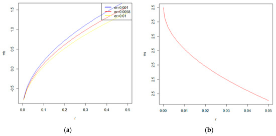
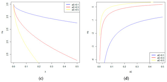
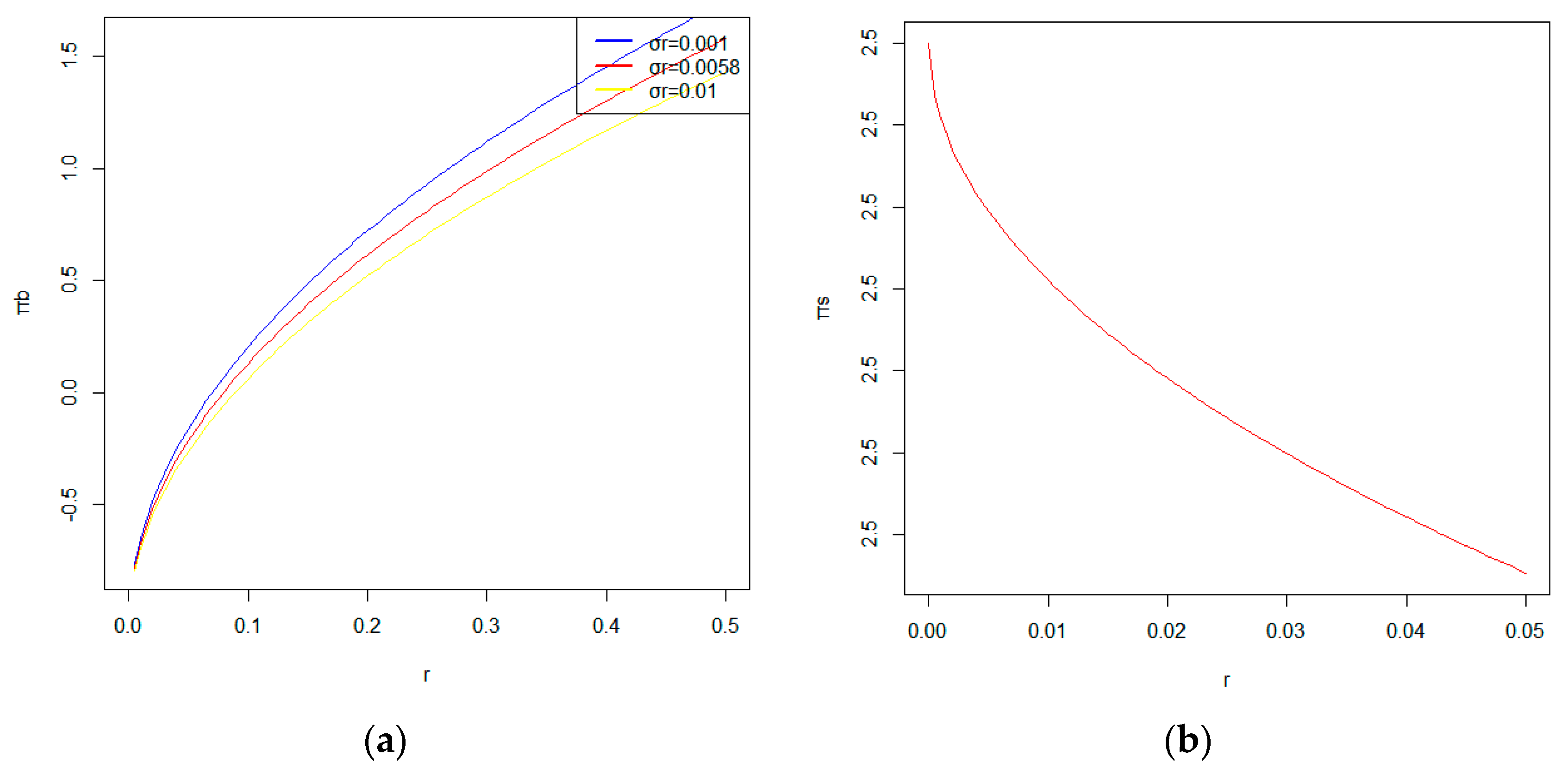
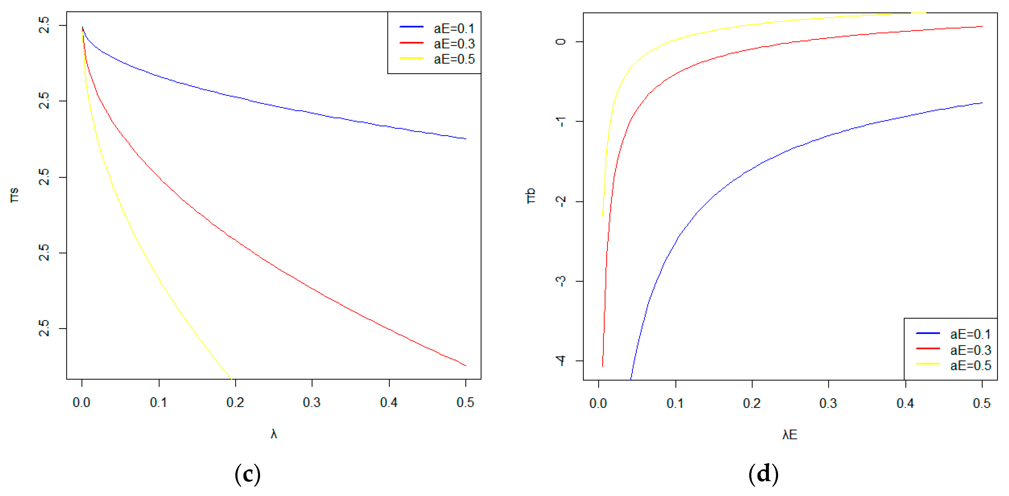
Figure 1a illustrates the changes in the optimal investment proportion of financial products under different volatilities of the risk-free interest rate. Keeping other conditions constant, as the risk-free interest rate increases, the optimal proportion invested in financial products also increases. With the rise in the risk-free interest rate, people are more willing to allocate more funds to purchase financial products driven by stochastic interest rates, expecting higher returns than those from risk-free assets. However, when the volatility of the stochastic interest rate increases, due to the heightened uncertainty in interest rate fluctuations, people tend to reduce their investment in interest rate-driven financial products, thereby mitigating the investment risks caused by interest rate volatility. This aligns with real-world observations. Additionally, we observe that the curve exhibits a diminishing marginal utility trend. As the interest rate continues to rise, the optimal proportion invested in financial products shows a marginal decline due to the increasing proportion allocated to risk-free assets. This is because, as the risk-free interest rate increases, these interest rate-driven financial products tend to resemble risk-free assets. When the risk-free interest rate reaches a certain level, the financial products become more akin to conservative income-generating financial instruments.

Figure 1b describes the changing trend of the optimal investment proportion of risk assets with interest rates. From the figure, we can directly observe that when the risk-free interest rate increases, the proportion of investment in risky assets continuously decreases. That is, people are more inclined to invest more assets in risk-free assets and wealth management products to obtain risk-free returns, which is consistent with reality. Secondly, when the interest rate volatility changes, we find that all the curves overlap, indicating that the impact of interest rate fluctuations on the optimal investment proportion in risky assets is very small. It also shows that after adding interest-rate-driven wealth management products, the fluctuations in the interest rate will more significantly affect the investment proportion between risk-free assets and wealth management products, which also corroborates the conclusion obtained from Figure 1a.

Figure 1c shows the variation of the optimal investment proportion in risky assets with changes in expected unexpected expenses. From the figure, we can see that as the expected future expenses increase, households face increasing risks of unexpected expenses and investment risks during the investment period. Firstly, to ensure that there will be sufficient funds to cope with unexpected expenses in the future, the purchase of risky assets will be reduced. That is, the purchase proportion of risky assets is sensitive to changes in the expectation of unexpected expenses, which is consistent with the research results of Yuan and Lai [20]. Secondly, as the volatility of random expenses increases, the sensitivity of the decline in the purchase proportion of risky assets also increases. That is, as the maximum unexpected expenses brought about by future uncertainties increase, people are reluctant to bear investment risks and are more willing to purchase risk-free assets.

Figure 1d depicts the variation of the optimal investment proportion in wealth management products under different degrees of random expenditure volatility. As the expected expenditure increases, from the analysis of the results in Figure 1c, we know that people will reduce their investment in risky assets. And this part of the endowment will be invested in wealth management products and risk-free assets to reduce investment risks and obtain risk-free returns. When the expected expenditure reaches a certain level, the optimal proportion of investment in wealth management products tends to a certain fixed value, which also indicates that an increase in expected expenditure may lead to the possibility of family investment bankruptcy.

The discussions above, concerning the alterations in strategies due to parameter shifts, have deepened our comprehension of how modifications in key parameters influence real-world decision making, specifically the adjustments in the optimal investment ratio and investors’ decision making [23].

5. Conclusions

In the family portfolio planning problem, there is one risk-free asset, multiple risky assets, and one wealth-management product in the financial market. Assume that the interest rate of the risk-free asset is set as a stochastic interest rate, the risky assets follow a multi-dimensional geometric Brownian motion process, and each family faces an uncontrollable stochastic expenditure risk process with jump-diffusion characteristics. A target function for maximizing the terminal value is established. Through the dynamic programming method, the HJB equation is derived. By using the Legendre transformation and the dual transformation, under the HARA utility function, an explicit solution for an optimal investment strategy is obtained. Finally, a numerical example is used to analyze the impact of various parameters on the optimal strategy. The results show that changes in the stochastic interest rate can affect the optimal investment proportion. As the risk-free interest rate increases, the optimal proportion of investment in wealth-management products also increases, while the proportion of investment in risky assets continuously decreases. As the expected future expenditure increases, families will reduce the purchase of risky assets, and the purchase proportion of risky assets is sensitive to changes in the expectation of unexpected expenditures. Moreover, during the investment period, families not only face investment risks but also expenditure risks brought by exogenous cash flows. The different correlations between the two can lead to changes in the family’s optimal investment strategy, thus achieving risk hedging. These conclusions have certain guiding and practical significance in practice.

In this paper, we compare our findings with the previous literature on the portfolio optimization problem, particularly when considering stochastic interest rates. We demonstrate that different initial interest rates affect the optimal investment ratio, and that this impact follows a trend and logic consistent with real-world scenarios. Furthermore, in the context of investing in risky assets with stochastic volatility, we explain how changes in the volatility of these assets influence the optimal investment ratio. When stochastic expenditure risk is taken into account, the paper also elaborates on how the optimal allocation decisions of households shift due to varying expectations of future expenditure risk. These optimal investment ratios are more reflective of actual household investment behaviors. Future research will persist in refining the problem of optimal household investment strategies under stochastic expenditure, enhancing the depiction of financial markets, incorporating a life-cycle theory framework, and more comprehensively analyzing the wealth change processes at different life stages to continuously enhance this area of research.

References

- Lu, X.; Li, Y.; Gan, L.; Wang, X. Risks in Chinese household financial portfolios—Too conservative or too aggressive? Manag. World 2017, 12, 92–108. [Google Scholar]
- Liu, Y.; Zhang, W.; Zhang, P. A multi-period portfolio selection optimization model by using interval analysis. Econ. Model. 2013, 33, 113–119. [Google Scholar] [CrossRef]
- Ferland, R.; Watier, F. Mean-variance efficiency with extended CIR interest rates. Appl. Stoch. Models Bus. Ind. 2010, 26, 71–84. [Google Scholar] [CrossRef]
- Chang, H.; Rong, X.; Zhao, H. Asset—Liability management model based on quadratic utility maximization under CEV model. J. Eng. Math. 2014, 31, 112–124. [Google Scholar]
- Guan, G.; Liang, Z. Optimal-management of DC pension plan in a stochastic interest rate and stochastic volatility framework. Insur. Math. Econ. 2014, 57, 58–60. [Google Scholar] [CrossRef]
- Chang, H.; Chen, X. Defined Contribution Pension Planning with the Return of Premiums Clauses and HARA Preference in Stochastic Environments. Acta Math. Appl. Sin. 2023, 39, 396–423. [Google Scholar] [CrossRef]
- Zhao, H.; Rong, X. Portfolio selection problem with multiple risky assets under the constant elasticity of variance model. Insur. Math. Econ. 2012, 50, 179–190. [Google Scholar] [CrossRef]
- Chang, H.; Rong, X.M.; Zhao, H.; Zhang, C.B. Optimal investment and consumption decisions under the constant elasticity of variance model. Math. Probl. Eng. 2013, 2013, 974098. [Google Scholar] [CrossRef]
- Bakkaloglu, A.; Aziz, T.; Fatima, A.; Mahomed, F.M.; Khalique, C.M. Invariant approach to optimal investment-consumption problem: The constant elasticity of variance(CEV) model. Math. Methods Appl. Sci. 2017, 40, 1382–1395. [Google Scholar] [CrossRef]
- Rong, X.; Fan, L. Optimal Investment Strategy of Insurers under Long Elastic Variance Model. Syst. Eng. Theory Pract. 2012, 32, 2619–2628. [Google Scholar]
- Gu, M.; Yang, Y.; Li, S.; Zhang, J. Constant elasticity of variance model for proportional reinsurance and investment strategies. Insur. Math. Econ. 2010, 46, 580–587. [Google Scholar] [CrossRef]
- Li, Q.; Gu, M.; Liang, Z. Optimal excess-of-loss reinsurance and investment polices under the CEV model. Ann. Oper. Res. 2014, 223, 273–290. [Google Scholar] [CrossRef]
- Lin, X.; Li, Y. Optimal reinsurance and investment for a jump diffusion risk process under the CEV model. N. Am. Actuar. J. 2011, 15, 417–431. [Google Scholar] [CrossRef]
- Huang, H.; Milevsky, M.A. Portfolio choice and mortality-contingent claims: The general HARA case. J. Bank. Financ. 2008, 32, 2444–2452. [Google Scholar] [CrossRef]
- Jung, E.; Kim, J. Optimal investment strategies for the HARAutility under the constant elasticity of variance model. Insur. Math. Econ. 2012, 51, 667–673. [Google Scholar] [CrossRef]
- Bo, L.; Li, X.; Wang, Y.; Yang, X. Optimal Investment and Consumption with Default Risk: HARA Utility. Asia-Pac. Finan Mark. 2013, 20, 261–281. [Google Scholar] [CrossRef]
- Chang, H.; Chang, K.; Lu, J. Portfolio Selection with Liability and Affine Interest Rate in the HARA Utility Framework. Abstr. Appl. Anal. 2014, 2014, 312640. [Google Scholar] [CrossRef]
- Nie, G. Optimal reinsurance and investment strategy to maximize HARA utility under CEV model. Math. Pract. Underst. 2019, 49, 249–255. [Google Scholar]
- Zhang, Y.; Wang, Z. Optimal Investment-Reinsurance Strategy Problems Based on the HARA Utility Function under the Ornstein-Uhlenbeck (O-U) Model. Chin. J. Eng. Math. 2024, 41, 915–930. [Google Scholar]
- Yuan, W.; Lai, S. Family optimal investment strategy for a random household expenditure under the CEV model. J. Comput. Appl. Math. 2019, 354, 1–14. [Google Scholar] [CrossRef]
- Mirkov, N.; Fabiano, N.; Nikezić, D.; Stojiljković, V.; Ilić, M. Symmetries of Bernstein Polynomial Differentiation Matrices and Applications to Initial Value Problems. Symmetry 2024, 17, 47. [Google Scholar] [CrossRef]
- Jane, K.; Shreve, S. Asymptotic analysis for optimal investment and consumptioncosts. Financ. Stoch. 2004, 8, 181–206. [Google Scholar]
- Xiao, G.; Hayat, K.; Yang, X. Evaluation and its derived classification in a Server-to-Client architecture based on the fuzzy relation inequality. Fuzzy Optim. Decis. Mak. 2023, 22, 213–245. [Google Scholar] [CrossRef]
Disclaimer/Publisher’s Note: The statements, opinions and data contained in all publications are solely those of the individual author(s) and contributor(s) and not of MDPI and/or the editor(s). MDPI and/or the editor(s) disclaim responsibility for any injury to people or property resulting from any ideas, methods, instructions or products referred to in the content. |
© 2025 by the authors. Licensee MDPI, Basel, Switzerland. This article is an open access article distributed under the terms and conditions of the Creative Commons Attribution (CC BY) license (https://creativecommons.org/licenses/by/4.0/).