Predicting the Distribution of Ailanthus altissima Using Deep Learning-Based Analysis of Satellite Imagery

Abstract

Invasive species negatively affect ecosystems, economies, and human health by outcompeting native species and altering habitats. Ailanthus altissima, also known as the tree of heaven, an invasive species native to China that has spread to North America and Europe. Commonly found in urban areas and forestland, these invasive plants cause ecological and economic damage to local ecosystems; they are also the preferred host of other invasive species. Ecological stability refers to the balance and harmony in species populations. Invasive species like A. altissima disrupt this stability by outcompeting native species, leading to imbalances, and there was a lack of research and data on the tree of heaven. To address this issue, this study leveraged deep learning and satellite imagery recognition to generate reliable and comprehensive prediction maps in the USA. Four deep learning models were trained to recognize satellite images obtained from Google Earth, with A. altissima data obtained from the Life Alta Murgia project, LIFE12 BIO/IT/000213. The best performing fine-tuned model using binary classification achieved an AUC score of 90%. This model was saved locally and used to predict the density and probability of A. altissima in the USA. Additionally, multi-class classification methods corroborated the findings, demonstrating similar observational outcomes. The production of these predictive distribution maps is a novel method which offers an innovative and cost-effective alternative for extensive field surveys, providing reliable data for concurrent and future research on the environmental impact of A. altissima.

1. Introduction

When an invasive species is introduced, the non-native organism, whether an insect, parasite, plant, or animal, begins to spread and reproduce from the site of its introduction [1]. This dissemination can lead to deleterious effects on the well-being of the environment, resulting in ecological and economic damage and threats to the health of native species [2,3]. The impact of an invasive species can disrupt the balance of the native ecosystem and its biodiversity. Native species that are killed or outcompeted may lead to potential extinctions across the ecosystem [2]. Indeed, invasive species have contributed to at least 42% of the decline in the endangered species population worldwide [4]. In the USA, these deleterious invasive species are widespread across various ecosystems. The consequences include severe issues, such as a reduction in crop production, the obstruction of waterways and drains, disease transmission among animals and even humans, and an increased risk of extreme climates [5]. In urban areas, invasive plants even have the potential to affect the environment and public health [3]. In general, invasive species tend to disrupt ecological stability and creating imbalances in biodiversity. A disruption like such upsets the harmony of the ecosystems.

A variety of management methods have been used on invasive species, particularly invasive plants [6,7]. Researchers and forestland owners typically adhere to established protocols for handling invasive species, which include evaluating the steps in determining the effect of human intervention on the environment, with methods ranging from biological to chemical. Additionally, protocols entail surveying for the exact locations of the invasive plant [8]. Federal agencies reported spending more than half a billion dollars per year in the early 2000. And approximately half those expenses were spent on preventions. Several states also spent a significant amount of resources on managing non-native species [9]. A 2021 study estimated that the problems of invasive species cost North America USD 2 billion per year in the early 1960s to over USD 26 billion per year since 2010 [10]. And globally, invasive species have caused a loss of USD 1.288 trillion over the past 50 years [11]. Traditionally, the detection of invasive plants has been based on in-field surveys and manual inspections. However, these practices present challenges: forestland owners must navigate management strategies that could even potentially increase the invasiveness of the species. Simultaneously, the demanding nature of regular monitoring may discourage engaging in invasive plant surveying or removal due to the intensity of work required by regular monitoring [6]. The consequent data obtained could be burdened by certain limits such as workload, area accessibility, and the efficiency of invasive plant detection. Consequently, conducting in-field surveys can be unproductive and costly [7]. All these factors call attention to the complex challenges in managing invasive plant species, emphasizing the need for efficient, cost-effective, and less labor-intensive methods for detection and management.

One such method of facilitated monitoring is using artificial intelligence and remote sensing along with satellite images. Using artificial intelligence and remote sensing, researchers can efficiently provide valuable information for further research [12], as shown in the study of Bibault et al. [13], in which cancer prevalence data from more populated areas (such as cities) were obtained and utilized alongside satellite images for deep learning feature extraction and prediction. The primary objective of their study was to provide a comprehensive prediction map of cancer prevalence in less populated areas where cancer data were inaccessible. The predicted outcome maps were illustrated for seven of the most populated cities to validate their model. Other similar studies further demonstrate that the application of remote sensing and satellite imagery is beneficial for reducing survey costs and increasing survey efficiency [12,14,15]. In addition to lowering survey costs, remote sensing techniques can allow researchers to obtain surveys of dangerous study areas, such as tiger reserve studies [15]. Studies have also demonstrated the use of remote sensing and satellite imagery to detect invasive species [7,14,15,16,17,18]. By utilizing methods such as deep learning, the resulting maps show patterns that can be interpreted as the “spatial symmetry” of its distribution [19]. The density maps generated represent a form of mathematical symmetry, as they map regions where the species thrives, helping to quantify and monitor ecological changes in a structured and predictable way. An example of such symmetry in studying the spread of an invasive species would be when an invasive plant species is introduced to a perfectly flat and homogeneous grassland; the seeds of the plant would begin to spread evenly in all directions due to uniform wind patterns and equal soil conditions. The spatial symmetry here lies in the even, radial distribution of the plant across the landscape. Our approach involves a novel, state-of-the-art methodology that combines advanced computer vison techniques (i.e., convolutional neural networks and vision transformers) to create remote sensing prediction maps.

Ailanthus altissima (Mill.) Swingle, commonly known as the “Tree of Heaven”, is a notable example of an invasive species. Native to China and Northern Vietnam, this species has extended its invasive reach to Europe, North America, and all continents besides Antarctica [20]. A. altissima is most commonly found in urban settings and along roadsides [21], but can also thrive in various other habitats, including forest edges and grassy fields [4]. A. altissima has a wide tolerance to different soil conditions and pollution, in addition to being resistant to drought and dry areas, making it highly suitable for urban environments [20,22]. Moreover, A. altissima produces chemical compounds that make it resistant to herbivorous predators and pathogenic diseases. Its allelopathic properties enable it to release toxic chemicals into the soil, thereby killing or damaging native plant species [5]. The combination of resistance to weather and the surrounding environment, along with defensive mechanisms, allow A. altissima to attain reproductive success and become highly invasive [20]. In addition to causing ecological damage, A. altissima also serves as a host plant for numerous pests and insects, including the spotted lanternfly, adding to its negative impact on invaded ecosystems [23]. Therefore, the invasive A. altissima yields deleterious environmental and economic effects. The challenge posed by the invasiveness of A. altissima necessitates concerted efforts in management and control. Various strategies have been employed to combat the invasion of A. altissima, including physical removal, chemical treatments, and the introduction of biological control agents. However, the effectiveness of these methods can be inconsistent and often requires ongoing monitoring and intervention. As a result, remote sensing techniques and satellite images have been employed to detect A. altissima. Both methods have been used for A. altissima geospatial predictions [14]. A semantic segmentation approach using older deep learning models was utilized to study the Alta Murgia National Park region in Italy [14]. Previous studies have demonstrated the effectiveness of machine learning and remote sensing to monitor invasive plants [24,25]. Other studies, such as those by Tarantino and Rebbeck [14,18] have shown interest in monitoring invasive A. altissima. Other studies [26] have also demonstrated the use of satellite imagery, remote sensing and CNN models for prediction. The combination of public and accessible satellite images with traditional machine learning has been shown to be an effective method for plant- and geospatial-related data management, which could be applied to study A. altissima. The combination of public and accessible satellite images with traditional machine learning has been shown to be an effective method for plant- and geospatial-related data management, which could be applied to study A. altissima. Our study differs from previous studies in the comprehensiveness and novelty of A. altissima prediction as we utilized four different supervised learning models, as well as two different classification methods, incorporating the method of inference testing in the United States. As opposed to previous studies using only a convolutional neural network (CNN) and a simple CNN framework to conduct remote sensing, our study incorporated a comparison of multiple CNN models, as well as a state-of-the-art vision transformer model [17]. Compared with the new state-of-the-art transformer models, the CNN frameworks have served as the backbone of the computer vision tasks. Transformers, originally designed for NLP (natural language processing) tasks, have shown promising and competitive results for CNNs in those computer vision tasks, such as the ViT (vision transformer) [27]. Compared to previous studies only utilizing datasets from one area, our study combined satellite images and surveys from different regions to comprehensively generate prediction results. Our study also employed novel methods to validate our results, including the use of multi-class classification and population density graphs along with tree cover graphs. Our method is novel due to the implementation of the remote sensing method on invasive species prediction and comparing a variety of models together for a comprehensive prediction on the spread of the tree of heaven.

Considering the invasive nature of A. altissima and the notable gap in predictive research within the U.S., our study focuses on the application of remote sensing techniques to track this species’ spread across American landscapes. Owing to the deleterious effects of A. altissima, coupled with a lack of comprehensive data and public surveys, the need for an accurate prediction model remains. Our objective is to develop an innovative method using convolutional neural networks (CNNs) to predict and monitor the spread of A. altissima, aiming to create a detailed prediction map. This approach is expected to minimize the costs and efforts involved in traditional surveying and management practices if not eliminated. In this study, we hypothesized three predictions: (1) using multi-class classification will yield similar mapping results as the binary classification method due to utilizing the same models and datasets, (2) the A. altissima distribution in the USA would closely follow the distribution of roads or forest land visible on satellite images because the distribution of the invasive plant follows that of human activities, and (3) the CNN will yield the most accurate results compared with the vision transformer due to the fundamental structural difference between the two. To test these hypotheses, we utilized data and information from Alta Murgia National Park and satellite imagery. The outcomes of this study could provide guidance for future research on invasive species, generate detailed and accurate indices for urban green space planning, and improve urban development.

2. Materials and Methods

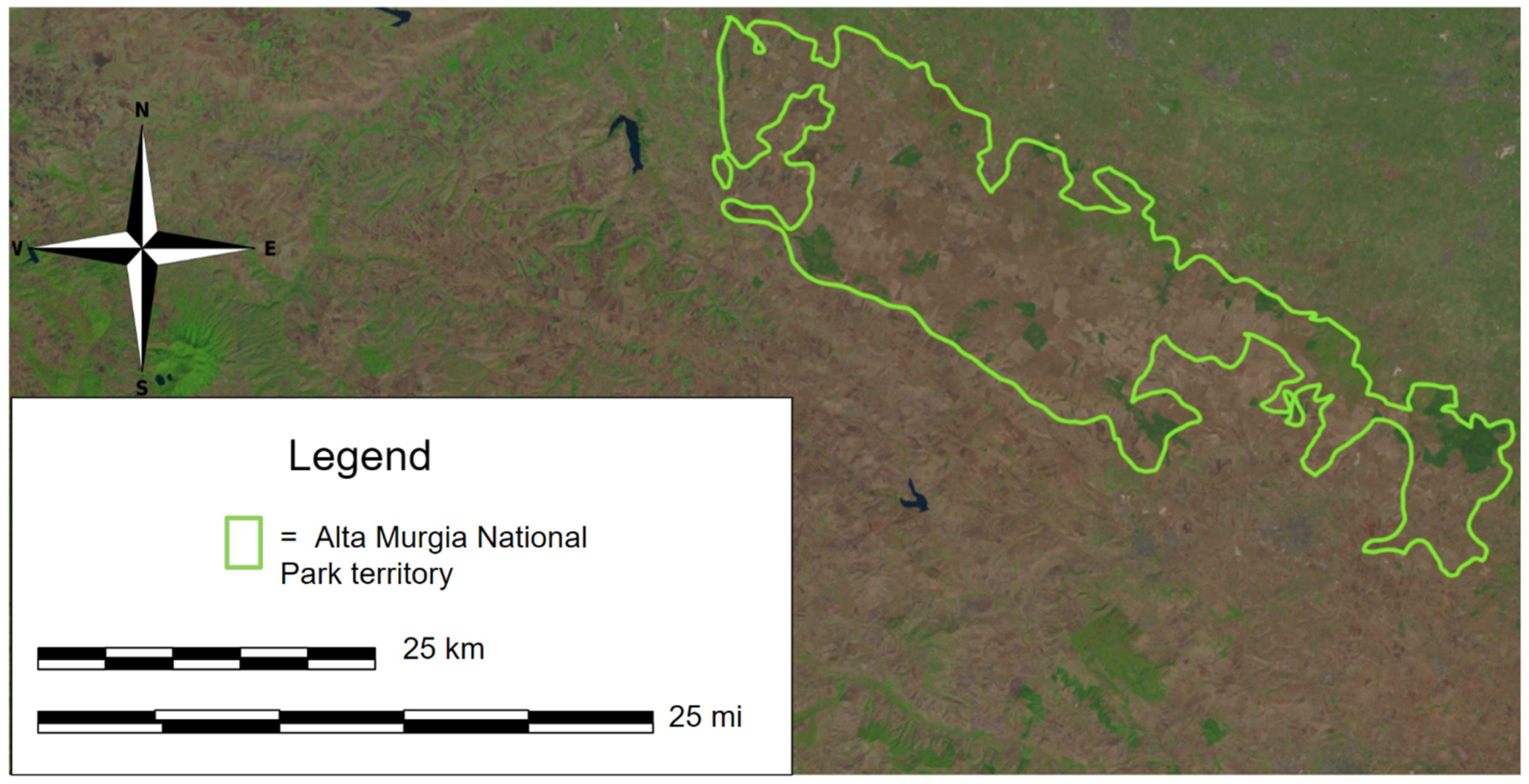
Section 2 is divided into four sub-sections: study area, data source, model frameworks, and the experimental procedure. Section 2.1 provides a detailed description of the target area, Alta Murgia National Park, as well as the state of New Jersey, and the importance of both areas in the scope of this study. Section 2.2 provides a summary of the data used in this study. Section 2.3 presents the framework of the models selected in our experiment. Lastly, Section 2.4 provides a detailed framework for the procedure of our experiment.

2.1. Study Area

In this study, ground truth data were obtained from an area located in Alta Murgia within the Apulia region of Southern Italy. Protected sites from the European Natura 2000 network include sites for endangered and rare species, supporting crucial habitat types, such as natural dry grasslands [14]. National parks support the conservation of birds, priority species, and wildfires. With the proliferation of A. altissima, national parks are prone to greater pressures and the danger of destruction [28]. Owing to the lack of data in the USA, we used professional mapping conducted in Alta Murgia National Park as the ground truth. Figure 1 illustrates satellite imagery of the target area of Alta Murgia National Park.

For the data inferencing procedure, we chose the state of New Jersey for the prediction. New Jersey is infested with A. altissima, as well as other invasive plants and insects. Satellite images were obtained for both Alta Murgia National Park and New Jersey. Training, testing, and validation using a CNN were performed on tiled satellite images with the exact coordinates of the surveyed locations of A. altissima. Geospatial maps were created based on the results of data inference in New Jersey.

2.2. Data Source

Two types of data were obtained: the exact coordinates of A. altissima in Alta Murgia National Park region and Google Earth satellite images. The sources of both types of data are described below.

The exact coordinates of A. altissima were obtained from Alta Murgia National Park, reported, and mapped, as surveyed by the Life Alta Murgia Project [29]. With more than 400 reported sightings in this area, we downloaded the corresponding satellite images captured before 2012 (the year the survey was conducted) and performed data processing before using CNNs. The original EDDMaps.org dataset and other datasets were used to demonstrate a statistical correlation with the SLF distribution [30,31]. A previous attempt to use data downloaded from EDDMaps.org for ground truth included reported sightings appearing to be extremely “noisy” and unsystematic. Many of the data documented spanned from different timelines, some with over a decade’s interval from each other. And if we were to incorporate the data assuming each marking occurred in the same period, it would have resulted in an inaccuracy in the prediction of our models.

The second type of data (Google Earth Satellite images) was obtained from publicly available Google Earth satellite images of Alta Murgia National Park and the state of New Jersey. Each region was tiled into smaller images and saved locally with 400 × 400 pixels at the 18th resolution (1:4513). Each image had a standard conversion of 0.90 m/pixel [32]. Distribution and prediction maps of other data sources in the United States were also used for final validation, such as tree canopy cover and population density maps [33,34].

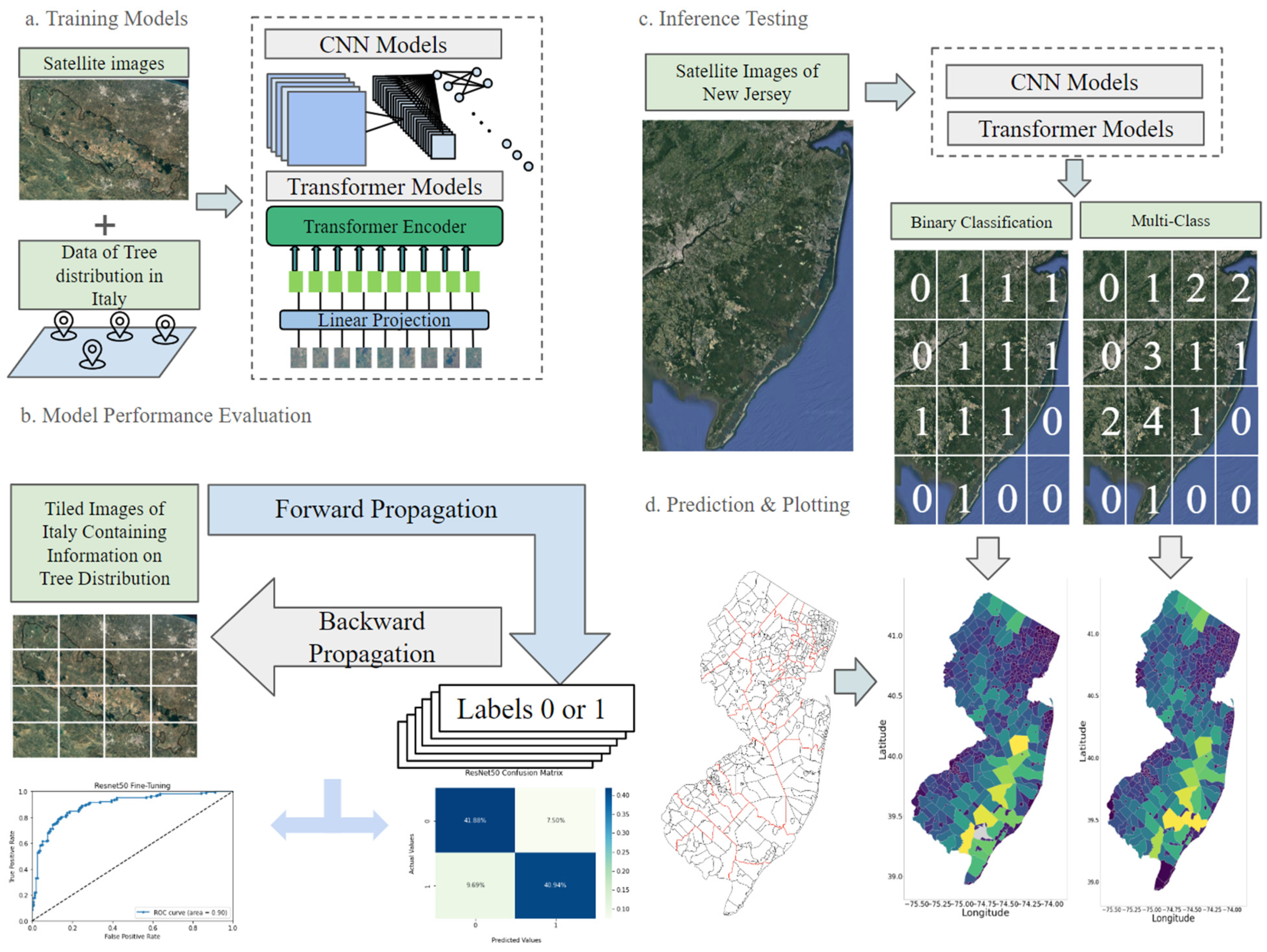
2.3. Model Frameworks

In this study, three convolutional neural network models were utilized along with one vision transformer model with weights pre-trained on the benchmark dataset ImageNet. The models used were ResNet50, EfficientNetv2, VGG16, and the vision transformer (ViT). Three out of the four models convolutional neural networks. We selected ResNet50 due to the residual neural networks, commonly known as ResNets neural networks, that apply “identity mapping”; the input of some layers is passed directly to other layers [35]. The benefits of using ResNet50 are its ability to be trained with thousands of layers with ease without raising the training error percentage and the ability to solve the vanishing gradient problem using “identity mapping”. As Gao mentioned in their research on determining critical lung cancer subtypes from gigapixel multi-scale whole slide H&E-stained image, ResNet50 had the highest overall performance with an area under curve (AUC) score of 1.000 and an accuracy score of 0.998.

Aside from conventional convolutional neural networks, we selected EfficientNetv2 for its state-of-the-art training speed and parameter efficiency. A relatively new model, EfficientNetv2, is aimed at optimizing training speeds and including new convolutional blocks, such as Fused-MBConv; it is up to 6.8x faster than previous models [36,37].

We also selected vision transformers, or ViTs, as an alternative to using CNNs for binary/multi-class predictions. Originally designed to help language translations, vision transformers enable modeling between input sequence elements. Vision transformers apply self-attention modules, a type of attention mechanism complementary to convolutions, and assist with multi-level dependencies across image regions [38]. ViTs and CNNs differ in their underlying structures and how they process input data. One noted drawback of using the ViT is its slow processing time [39].

Table 1. Summarization of the strengths and weaknesses of CNNs vs. ViTs.

Aspects	CNN	ViT
Architecture	Uses convolutional layers for local feature extraction.	Uses self-attention for global context and relationships.
Strengths	Efficient at capturing spatial hierarchies; faster training.	Handles global dependencies effectively.
Limitations	Struggles with global context without deep architectures.	Slower processing and higher computational demand.
Training	Relatively faster with optimized architectures.	Requires larger datasets and more resources.
Application	Satellite imagery classification (e.g., ResNet50, EfficientNet).	Alternative for classification with attention mechanisms.

summarizes the strengths and weaknesses of CNNs vs. ViTs.

The last model we selected was VGG16, the second-best performing model from Gao’s study on lung cancer binary classification [40], with AUC scores of 1.000 and 0.997 accuracy. A model developed in 2014 consists of a few basic layer types, which makes it easy to modify and adapt for fine-tuning different tasks [41]. The architecture has many parameters, which can be computationally challenging to train.

We established that between the two deep learning approaches of fine-tuning and representation learning [41], the benefits of using the fine-tuning methodology lie in its high accuracy because each models’ weights are continuously updated to fit the data, with the disadvantages of having an extremely high demand for computational power and being time-consuming. In contrast, using the feature extraction method along with a classifier, such as “logistic regression” or Support Vector Machines, for prediction demonstrated a significantly lower prediction accuracy, but a faster and more efficient computation time. For this experiment, we identified that accuracy outweighs the importance of more efficient computation ability. Thus, we used a fine-tuning approach for our binary classification labeling. After investigating the density predictions, we utilized feature extraction and fine-tuning for density-correlated predictions.

2.4. Experimental Procedures

The procedure of this experiment was as follows: First, image tiling and augmentation were performed in preparation for the training stage. Second, the training stage involved using four models to perform binary classification on the Alta Murgia dataset. Third, the data inferencing stage was applied in the trained models to satellite images of the USA. Lastly, owing to the lack of comparable studies conducted in the USA, we used multi-class prediction to validate our prediction results. Figure 2 demonstrates the workflow of this experiment.

2.4.1. Image Tilting and Augmentation

For our CNNs to successfully predict the images, each satellite image from an area must be downloaded at a high resolution and split into multiple grids with sizes of 400 × 400 pixels, along with a geotagging file in the “.kml” format. As our ground truth dataset consisted of satellite images from Alta Murgia, image tiling resulted in 25,000 images. Each image was subsequently tagged with a label of either “1” or “0” in reference to whether a data plot of the Alta Murgia tree exists within a tiled image. This was completed using simple iterations to test whether the coordinates (lat, long) were within the range of the corresponding geotagging file.

Data augmentation was performed after image tilting. Owing to the area limitation of the region, only 436 of the 25,000 images were marked as 1 (A. altissima present). The data imbalance present in the processed dataset can cause a severe imbalance in terms of testing, with one potential result being an altered value of false-negative percentages. As a result, approximately 400 random images from 21,000 data augmentations were performed; 400 more label 1 images were added to the dataset to increase the performance and accuracy of the data points. Studies have shown that data augmentation increases the ability of model generalization [42,43]. Some data augmentation techniques include altering the shape, orientation, and even colors of existing data to expand the variety of data collection fields [42]. Here, data augmentation focused on the quantity, rather than the quality, of the data, as the required classification performance was limited to satellite images. As the graphs below demonstrate, Figure 3a shows the AUC score before data augmentation, and Figure 3b shows the AUC score immediately after data augmentation. The results show that the prediction can be more accurate by utilizing this data approach.

2.4.2. Ground Truth and Binary Classification

The Alta Murgia plot data were utilized, along with satellite images, to train the three CNN models (pre-trained with ImageNet): ResNet50, EfficientNet, VGG16, and the ViT [35,36,37,38,44,45]. The following stages of this step involved binary classification and labeling each ground truth image from Alta Murgia National Park with either “1” or “0. Using the Life Alta Murgia, which contains approximately 400 coordinate plots, along with the corresponding satellite images, we created an HDF5 file with each satellite image resized to 224 × 224 × 3 and its corresponding label of either “0” or “1”; here, “0” signifies that no tree is present within that image and “1” indicates that the tree of heaven is present. Using a binary classification approach, we can guarantee a higher accuracy and achieve data granularity to a certain degree. HDF5, which stands for Hierarchical Data Format, stores the large amounts of data used for training, validation, and testing. Italian (Alta Murgia) data used as the ground truth underwent training, validation, and testing stages; the results of the testing stages indicated the performance of our models.

2.4.3. Inference Testing in USA

“Inferencing” in machine learning utilizes the knowledge it has learned from a neural network model with trained weights and uses it to infer a result [46]. In our case, as the existing data for A. altissima plotting in the USA are scarce and noisy, we used the state of New Jersey (which is known for the spread of spotted lanternflies) for prediction. Models trained using Alta Murgia National Park can be used to infer distributions in the USA. The best performing model (ResNet50) from the ground truth testing dataset was selected for inference testing in the USA.

Satellite images of New Jersey were stitched and downloaded from Google Earth at a resolution of 18 × (1:4513). Each image was tiled into sizes of 400 × 400, mirroring the sizes of the Alta Murgia images in the training and validation stages. The purpose of this process was to assign a corresponding binary label of “1” or “0”, indicating the presence or absence of the tree in each image and aggregating all the images that belong in a region (such as a county or municipality). A simple iteration was performed such that all available trees were tallied in each region, and the number was reported in a separate column for Python geospatial data plotting. Data inferencing was performed on each image with the methodology to obtain a series of prediction labels of either “0” or “1”, signifying the presence or absence of trees. Owing to the small size of each image, county-level predictions can equate each image’s prediction as representative of each area. The total number of trees present in each area represented the density of A. altissima across the state. The georeferencing files of all satellite images indicated the exact locations of each 400 × 400 image; thus, we could aggregate and calculate the average probability that the image contained the target. The numbers are represented on a geospatial map using the GeoPandas library. A shapefile of the state of New Jersey was obtained, and the county-level probability was calculated.

2.4.4. Multi-Class Classification Validation

Due to the lack of comparable datasets in the USA, we used a different validation method. Rather than using binary classification, we used multi-class classification to retrain our best-performing model (ResNet50) on the ground truth dataset and performed inference testing again using satellite images from New Jersey. If an observable similarity was observed between the two methods, the methodology could be validated. To do so, we started by following the same procedure as the probability prediction maps by aggregating and counting all the images labeled with “1”. Unlike the probability prediction, no averages were obtained. Instead, the summation of the number of trees was documented and used to plot the geospatial data. Instead of binary (0 and 1), the classes represented the four classes defined by the number of trees, where 0 represents no trees, 1 represents 1–4 trees, 2 represents 4–8 trees, and 3 represents >8 trees. After evaluation, the four-class (multi-class) model underwent the same inference testing procedure as before.

2.5. Tools Utilized

This study was conducted on a device with Intel Core i7 12th Gen, 32 GB Ram, and NVIDIA GeForce RTX 3060 Ti. We utilized Jupyter Notebook to perform machine learning on the datasets, of which we used Python3.0 primarily for our study. We utilized libraries such as Matplotlib, Pandas, PyTorch, and GeoPandas, among others.

3. Results

Following the methods and procedures listed above, we obtained the following results: ground truth training and testing based on Alta Murgia, inference testing in New Jersey (resulting in prediction maps), and validation with multi-class prediction.

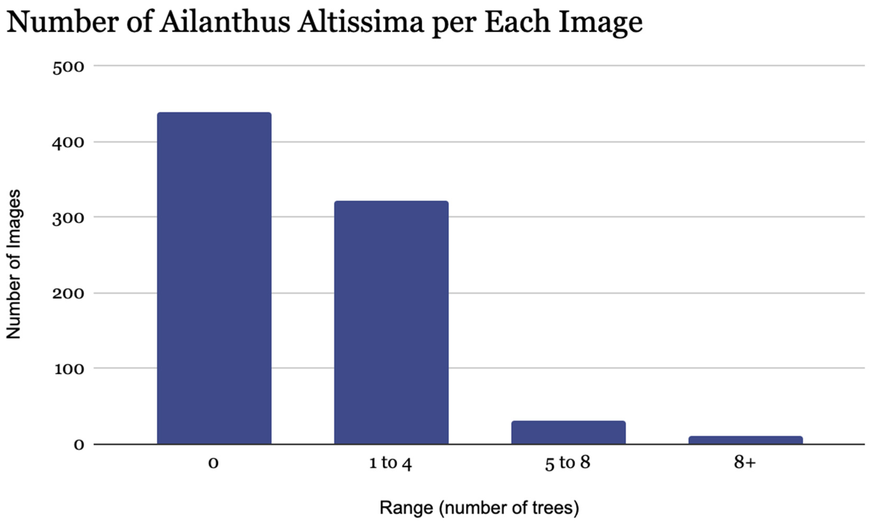
3.1. Ground Truth Result

After running eight batches at once for training, owing to computational limitations, we ran 100 epochs with a learning rate of 0.01 for each of the three models: ResNet50, EfficientNetv2, VGG16, and the ViT. After each iteration, the best performing models were saved locally for testing and later for inference testing in the USA.

Table 2. Performance of the four models.

Model Name	AUC Score	Accuracy	F1 Score
ResNet50	0.900	0.822	0.824
EfficientNetv2	0.880	0.793	0.778
ViT	0.868	0.781	0.780
VGG16	0.880	0.784	0.786

presents the AUC, accuracy, and F1 scores of each of the four models. The best performing model was ResNet50 with an AUC score of 0.900, whereas the worst performing model was the ViT with an AUC score of 0.868. Figure 4 provides a visual representation of the receiver operating characteristic (ROC) curves and the confusion matrix for each model, obtained using the fine-tuning approach, with the area under the curve (AUC) values displayed at the bottom right. All four curves closely approach the top-left corners of their respective graphs, consistently indicating that our models are effective in classifying satellite images into subcategories.

The two classes, 0 and 1, illustrate the first stage of the training procedure, in which the primary focus is to distinguish whether a tree exists in an image. Figure 4 and Figure 5 also illustrates the confusion matrices of all four with consistent and relatively low false negatives and false positives. This indicates that the datasets of our models were balanced, avoiding potential prediction inaccuracies. Out of the four models, the results of the three CNNs were significantly better than those of the ViT and feature extraction accompanied by logistic regression. ResNet50 performed the best out of the four models, with an AUC score of 0.900 and an accuracy score of 0.822. The ViT demonstrated the worst performance out of the four models, with an AUC score of 0.860 and an accuracy score of 0.784.

3.2. Inference Testing Result

We selected ResNet50, our best performing model, to perform inference testing on data from the USA. After careful validation, we chose to infer the state of the New Jersey density predictions using the models we previously built and saved. Next, we created multiple-density prediction maps, owing to the lack of validation of our inference testing. Following the procedure listed previously, Figure 5 shows the obtained results. Dark blue regions are low-tree-density areas while light yellow and green regions are high-tree-density areas. Both prediction maps illustrate a non-randomized distribution of the predicted A. altissima.

Compared with the county-level aggregation, the municipality-level prediction map illustrated a finer distribution of A. altissima. Fewer A. altissima were found in the top-right corner of the state, while the greatest number of A. altissima was found in the middle region. In contrast to the ground truth results, the inference testing results were qualitative and inferred from the observations of visual correlation.

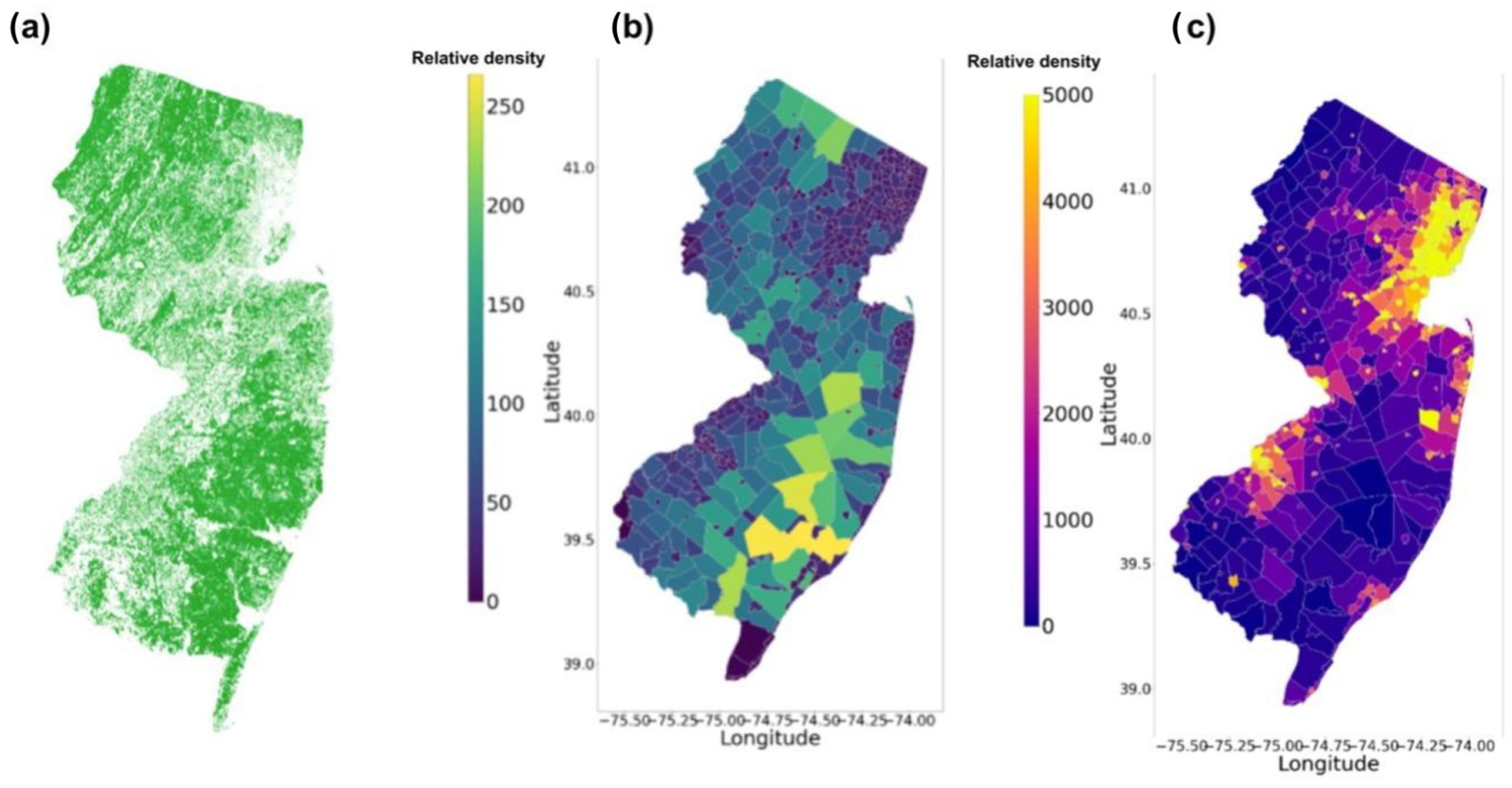
3.3. Feature Extraction Result

In addition to a binary classification approach, we also performed feature extraction along with logistic regression for multi-class prediction to evaluate the density of the Alta Murgia area. The previous image size was increased so that more trees were present in each image, as opposed to only 1 or 0. Each image size was enlarged such that each image had more land coverage, which in turn led to more A. altissima coverage. As a result, we could label each image not in a binary fashion, but more accurately in density. The presence of more trees in each image can contribute to an increase in the aggregation of each image and, therefore, more class predictions. As shown in Figure 6 the number of trees assigned to each image ranged from 0 to 10 depending on the distribution of the Alta Murgia tree survey coordinates. As previously mentioned, we summarized the trees into ranges of either 0, 1–4, 5–8, or >8 trees to increase the amount of data for each class. Feature extraction was performed using a pre-trained ResNet50 model, for which we achieved an accuracy of 0.73. The relatively low accuracy, compared with other contemporary works (such as Bibault’s prediction of cancer prevalence), could likely be attributed to the lack of data points and data imbalance in each class (in this case, the range of trees).

4. Analysis and Discussion

4.1. Validation of Inference Testing

As publicly available data for predictions are unavailable, we used our multi-class prediction models on New Jersey satellite images for prediction. By utilizing a different method for prediction (i.e., multiclass prediction), we compared the resulting graphs qualitatively to our previous testing results. If significant plotting overlaps could be observed, it could then be inferred that our predictions were validated.

In comparison with the binary classification method, we retained the characteristics of “classification” portion, as in we are still inputting different kinds of data for model classification. However, rather than labeling the results as either 0 or 1, we have multiple classes: 0 trees, 1–4 trees, 5–8 trees, and 8+ trees. We have also modified the range of our images such that a greater area will be covered with each image. We then summed up all the total trees within a certain area to calculate the density. The multiclass offers an additional method of verifying our methods of finding the density of the spread of the trees.

Both methods yielded similar results, and density mapping compensated for the lack of validation. A comparison of the result of the binary classification mapping to the multi-class classification mapping showed very similar shading and density results. Although the exact number of predicted densities varied, the results were still remarkably similar. This is likely attributable to the fact that in our binary classification approach, each image was aggregated with a smaller image size compared to multi-class classification. Although the exact density index on the index bar displayed a different range of numbers, the shading remained similar between the two methods, demonstrating that our models accurately represent the density between the regions.

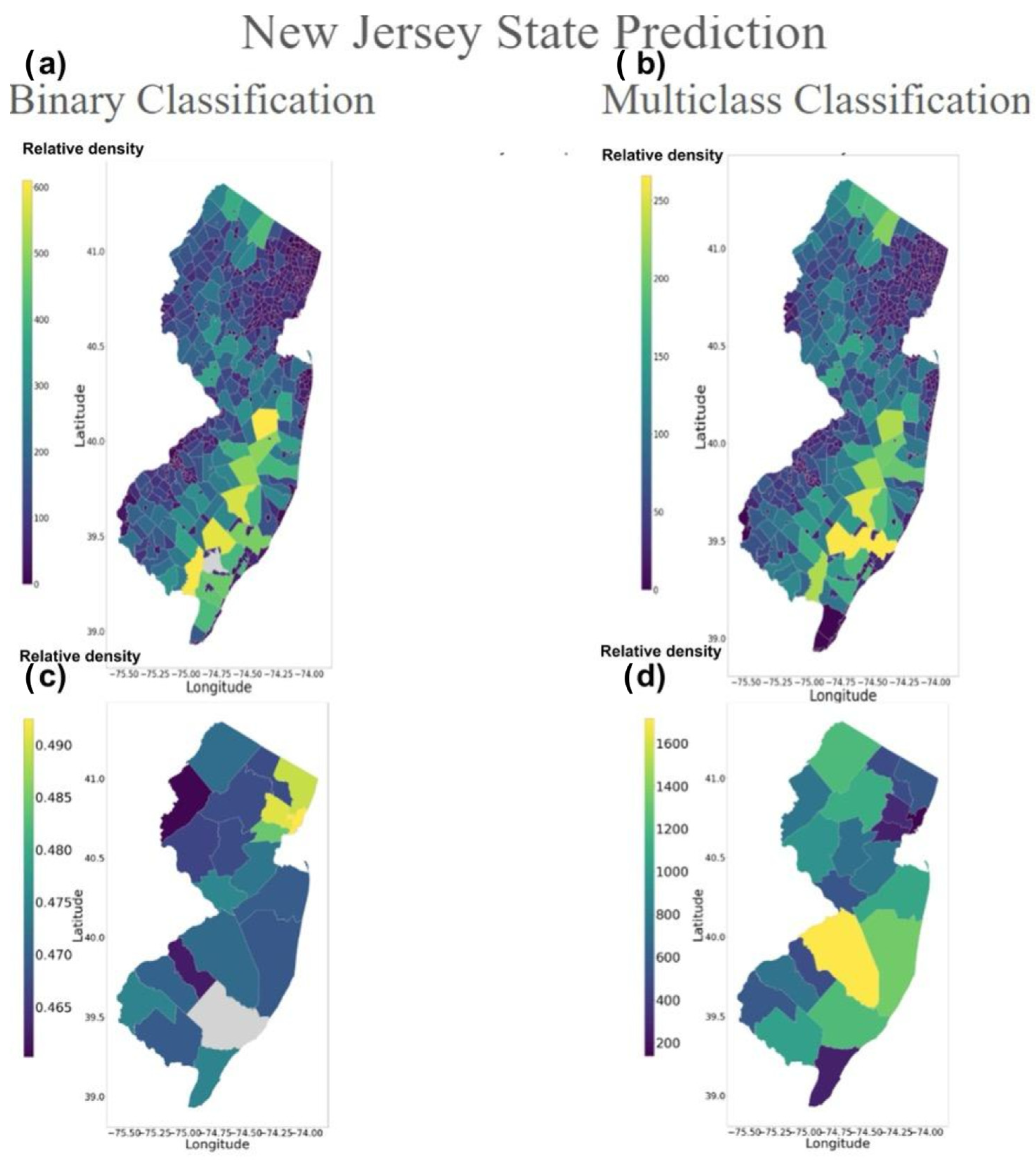
4.2. Analysis of Tree Distribution on New Jersey Prediction Map

The results of the experiment demonstrated the use of different image-processing models, from CNNs to vision transformers and from fine-tuning approaches to feature extraction. Although no validation of A. altissima in New Jersey is available, we could compare its density distribution with other density maps for New Jersey. For instance, our prediction maps showed some overlap with the forest land distribution and an inverse relationship with the population density of New Jersey. Our study aimed to determine a direct correlation between the spread of spotted lanternflies and that of A. altissima. Likewise, the spread of A. altissima could also be attributed to environmental factors, such as forest distribution or population locations.

Figure 7 shows the distribution of forest land in the state of New Jersey, with dark green areas as forests, sand-colored areas as non-forest, blue as water, and red-outlined regions as the Pinelands boundary. The map source was obtained as an overview of forest resources in New Jersey; it is based on an inventory by the USDA Forest Service, Forest Inventory and Analysis program, and Northern Research Station. The forest land distribution in the state of New Jersey could reflect the distribution of green tree crowns on the satellite images. Figure 6b illustrates our mapping of the A. altissima in the state of New Jersey using satellite images. We juxtaposed our data results against two other maps: the New Jersey forest land distribution (Figure 6a) and the New Jersey population density map (Figure 6c). Figure 6c illustrates the population density map of the state of New Jersey as a heatmap, where the warmer the hue is, the more populated the area. Likewise, the cooler the hue is, the less populated the area. Figure 6a was used to develop comparisons with our mapping results, exploring potential or existing correlations. Collectively, these three images show an observable correlation.

The less dense areas of A. altissima were mostly in urban areas, whereas the denser predicted areas of A. altissima were in forest regions. This could also potentially indicate that A. altissima has a high affinity for other forested vegetation types. Large forest land distribution is possibly scarce around more inhabited regions; such a correlation was reflected qualitatively and quantitatively in our prediction maps. Figure 8a indicates the spread of the forest land mapping in New Jersey, which inversely mirrors the distribution of the density population in New Jersey Figure 8c. Figure 8b illustrate our prediction of the spread of the Tree of Heaven. We have also performed a correlation analysis using the spearman method, which resulted in a −0.547 as a correlation value. This indicates that the population density and the tree of heaven density is inversely correlated. However, a contradiction was observed in A. altissima. In addition to woodland areas, these trees also inhabit urban areas, specifically roadsides, railways, and fences. However, our prediction indicated little to no A. altissima in populated areas. This could be attributed to the similarity of the crown of A. altissima to that of other common trees. In our model, which focuses on regional detection and summarization, the exact location can be missed during the training stages.

Furthermore, A. altissima growing in urban areas, specifically along crevices, is extremely small compared to the typical height of 60–80 feet. As a result, our models may have trouble locating invasive trees in satellite images of urban areas. One method to potentially overcome this issue is the use of semantic segmentation. Using semantic segmentation could potentially bridge some of the performance gap in our study, as semantic segmentation allows for better distinction between the A. Altissima and regular trees. By splitting the image into different segments and pixels, with some tree crowns labeled as A. altissima and others labeled as common trees, the prediction results could become even more accurate.

4.3. Analysis in Reference to Previous Studies

Similarly to Bibault’s study, our study focused on the primary objective of providing a sufficient and comprehensive model for predicting both the probability and density of A. altissima. Although the overall framework of our study was modeled after that of Bibault et al., the exact methodology was altered; a fine-tuning approach was utilized in this study as opposed to feature extraction and classification. A coordinate-level approach was implemented as opposed to county-level aggregation.

Our results, compared with similar studies using CNNs and satellite images for plants or invasive plant species, demonstrated a similar workflow but a difference in their application. Studies, such as those by Tarantino et al. and Lake et al. [14,16], have also shown an extra procedure of using semantic segmentation to help CNN models better pinpoint locations of A. altissima. Their models demonstrated a prediction accuracy of 96–80%. Without semantic segmentation, our models achieved accuracy scores between 78 and 82%. If we modified our framework and added more procedures, our accuracy score would most likely have increased by a margin.

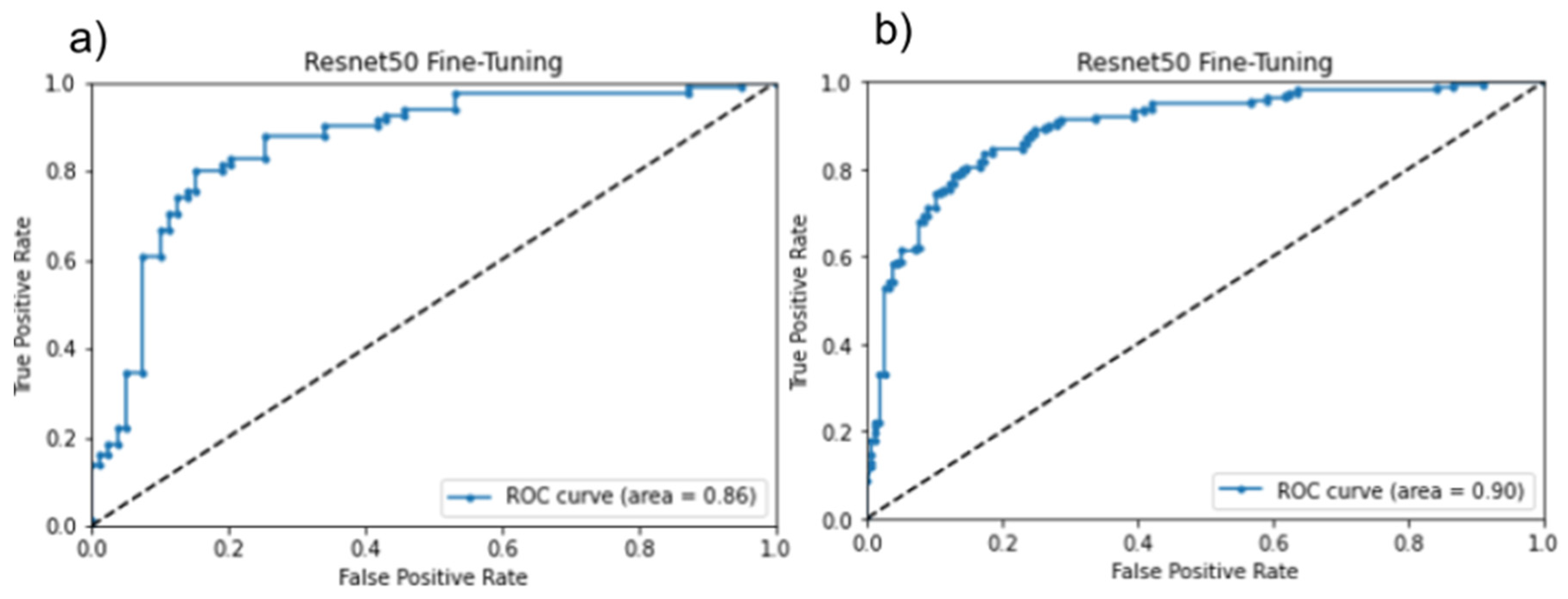
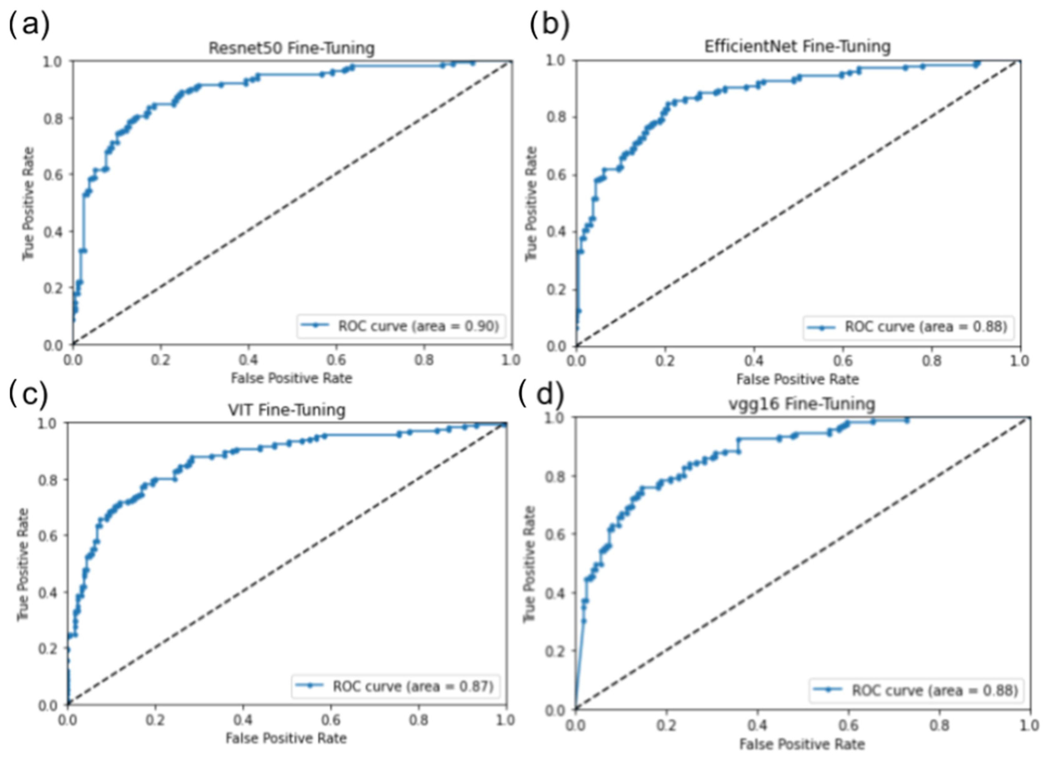
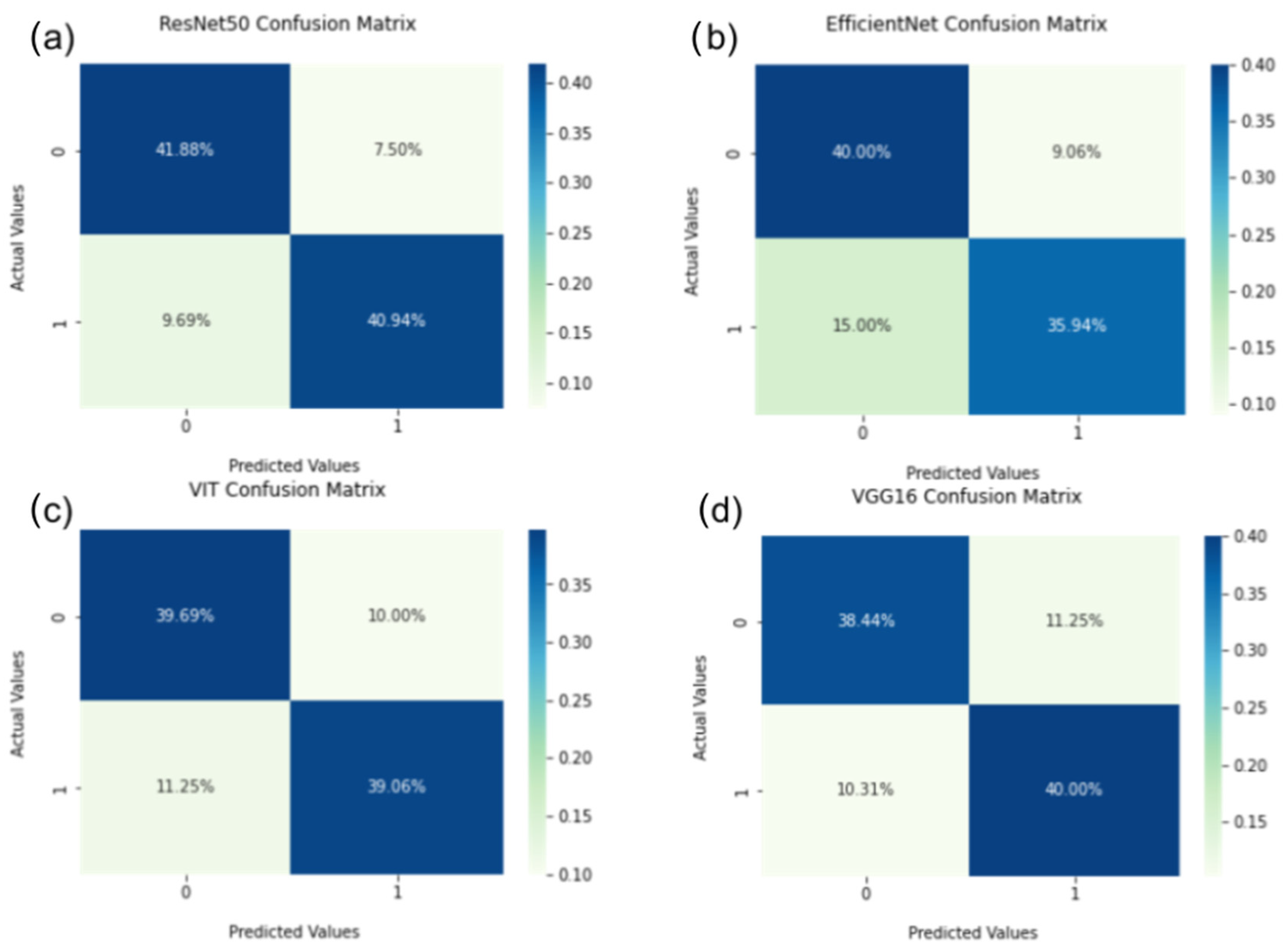
4.4. Machine Learning Performance Result Analysis

In our analysis, the three CNN models performed better than the ViT on all metrics (accuracy, F1 score, and AUC score). One of the goals of this study was to provide insights into the different models and state-of-the-art methods used in image analysis and classification.

Transformers were originally designed to assist in language translation because they enable the modeling of long dependencies and support parallel processing. Unlike CNNs, transformers utilize the concept of the attention mechanism because they enhance the important sections of the input data, whereas CNNs do not encode the relative positions of the features [39]. The vision transformer is an approach designed to replace CNN models. However, ViT training requires significantly more data than CNNs because CNNs encode knowledge about images, such as transitional equivariance, whereas the ViT must learn these properties from the provided data [47]. In our study, owing to the limited data obtained and provided, the ViT performance was better than that of the CNN.

Compared to Gao’s study on lung cancer binary classification using similar models and the same methods [40], the accuracy of the fine-tuning models showed a significant decline, while the feature extraction method remained at the same level of performance. This is likely attributable to the lack of data; we only had approximately 400 images for each binary class prediction, as opposed to Gao’s study, where 25,000 images were present for each binary class. The significant reduction in data size could lead to inaccuracy and higher precision and recall rates.

The data size limit also applies to the performance differences between binary/multi-class classification and feature extraction coupled with logistic regression. In Gao’s study, a relatively small data size led to a significantly higher accuracy (98–99% in binary classification and approximately 70% for the feature extraction method) in the binary classification methods, given that the models remained the same for both methods [40]. The same finding was also discovered in Gupta’s study on a comparison of using a pre-trained model versus the fine-tuning methodology [48]. Fine-tuning was significantly more accurate.

4.5. Limitations and Future Studies

This study was conducted on a personal computer with 32 GB of RAM; some machine learning functions, such as regression, could not be run locally. Computational limitations may have restricted data processing. Another limitation was the data imbalance. This issue was present during the beginning stages of our experiment: an imbalanced dataset can cause a severe imbalance during the testing stage, such as skewed false-negative percentages. Through data augmentation, the issue of data imbalance was resolved. In addition to the aforementioned limitations, we were hindered by the lack of available public data/surveys presenting the locations of A. altissima. Without validation from an external source, we used a different method to validate the inference-testing results.

In addition to harmful ecological damage, A. altissima is also a host plant for many pests and insects, one of which is the spotted lanternfly (SLF) species. Lycorma delicatula was first found in Pennsylvania, USA, in 2014. Native to China, these invasive plant hoppers use host plants, such as A. altissima, to lay larvae and nymphs [49]. Currently, 14 states and hundreds of counties are affected by SLF infestations. Although the exact ecological damage is unknown, the SLF is known to cause economic damage to vineyards, as well as local and state governments. The current solution proposed by the New Jersey state government is for citizens to kill as many flies as possible [50]. Consequently, there is an urgent need for accurate data. Our study provides a methodology consistent with the goal of reducing survey costs and provides future studies with a reliable source of information. Prediction maps of A. altissima could be used to predict the spread of the insect, as states in the vicinity, such as Massachusetts, New York, and Connecticut, have reported sightings of these insects [51,52,53].

5. Conclusions

By following the procedure and predicting the spread of A. altissima in the USA using satellite imagery, we verified our first hypothesis, i.e., multi-class prediction results in a prediction pattern similar to that of binary classification. Using the same dataset but a different method, we verified the consistency of our models. Although the distribution ranges were different, the correlated densities of the two maps were nearly identical. The predicted relative density can aid environmental scientists in studying the distribution of A. altissima in the context of its surroundings and ecosystems. We could also verify our second hypothesis that the predicted distribution of the invasive plant closely resembles the forest lands displayed on satellite imagery. One potential problem raised by this finding is that our models were perhaps unable to distinguish between regular forest ground satellite imagery and the regions of A. altissima. Nonetheless, this finding demonstrates that our models can associate features unique to each satellite image with the absence or presence of trees. However, although our prediction maps showed observable overlaps with the distribution of forest land in New Jersey, we discovered some portions of the regions showing a lack of forest land cover but a higher predicted A. altissima density. The lack of prediction maps and data complicates the validation process. Finally, as predicted, the CNN models performed significantly better than both the vision transformers and feature extraction (along with logistic regression) method. Our decision to use a range of models and methods validates the consistency of our results.

The fine-tuning methodology is highly accurate because each model’s weights are continuously updated to fit the data, with the disadvantages of an extremely high demand for computational power and time consumption. In contrast, using the feature extraction method, along with a classifier such as “logistic regression” or Support Vector Machines, for prediction demonstrated a significantly lower prediction accuracy, but a faster and more efficient computation time. In this experiment, we identified that accuracy outweighs the importance of more efficient computation ability.

References

1. Pyšek, P.; Richardson, D.M. Invasive Species, Environmental Change and Management, and Health. Annu. Rev. Environ. Resour. 2010, 35, 25–55. [Google Scholar] [CrossRef]
2. What Is an Invasive Species and Why Are They a Problem? U.S. Geological Survey. Available online: https://www.usgs.gov/faqs/what-invasive-species-and-why-are-they-problem (accessed on 27 July 2023).
3. Kumar Rai, P.; Singh, J.S. Invasive Alien Plant Species: Their Impact on Environment, Ecosystem Services and Human Health. Ecol. Indic. 2020, 111, 106020. [Google Scholar] [CrossRef] [PubMed]
4. Tree of Heaven (Ailanthus altissima): Invasive Species ID. Available online: https://www.nature.org/en-us/about-us/where-we-work/united-states/indiana/stories-in-indiana/journey-with-nature--tree-of-heaven/ (accessed on 27 July 2023).
5. Tree of Heaven; Invasive Species Centre: Marie, ON, Canada. Available online: https://www.invasivespeciescentre.ca/invasive-species/meet-the-species/invasive-plants/tree-of-heaven/ (accessed on 27 July 2023).
6. Wolde, B.; Lal, P. Invasive-Plant-Removal Frequency—Its Impact on Species Spread and Implications for Further Integration of Forest-Management Practices. Forests 2018, 9, 502. [Google Scholar] [CrossRef]
7. Sitzia, T.; Campagnaro, T.; Kowarik, I.; Trentanovi, G. Using Forest Management to Control Invasive Alien Species: Helping Implement the New European Regulation on Invasive Alien Species. Biol. Invasions 2016, 18, 1–7. [Google Scholar] [CrossRef]
8. Martin, P.A.; Shackelford, G.E.; Bullock, J.M.; Gallardo, B.; Aldridge, D.C.; Sutherland, W.J. Management of UK Priority Invasive Alien Plants: A Systematic Review Protocol. Environ. Evid. 2020, 9, 1. [Google Scholar] [CrossRef]
9. Warzinaick, T.; Haight, R.G.; Yemshanov, D.; Apriesnig, J.L.; Holmes, T.P.; Countryman, A.M.; Rothlisberger, J.D.; Haberland, C. Economics of Invasive Species. In Invasive Species in Forests and Rangelands of the United States; Springer: Cham, Switzerland, 2021. [Google Scholar] [CrossRef]
10. Crystal-Ornelas, R.; Hudgins, E.J.; Cuthbert, R.N.; Haubrock, P.J.; Fantle-Lepczyk, J.; Angulo, E.; Kramer, A.M.; Ballesteros-Mejia, L.; Leroy, B.; Leung, B.; et al. Economic Costs of Biological Invasions within North America. NeoBiota 2021, 67, 485–510. [Google Scholar] [CrossRef]
11. Zenni, R.D.; Essl, F.; García-Berthou, E.; McDermott, S.M. The Economic Costs of Biological Invasions around the World. NeoBiota 2021, 67, 1–9. [Google Scholar] [CrossRef]
12. Zhao, J.; Liu, X.; Kuang, Y.; Chen, Y.V.; Yang, B. Deep CNN-Based Methods to Evaluate Neighborhood-Scale Urban Valuation Through Street Scenes Perception. In Proceedings of the 2018 IEEE Third International Conference on Data Science in Cyberspace (DSC), Guangzhou, China, 8–21 June 2018; pp. 20–27. [Google Scholar] [CrossRef]
13. Bibault, J.-E.; Bassenne, M.; Ren, H.; Xing, L. Deep Learning Prediction of Cancer Prevalence from Satellite Imagery. Cancers 2020, 12, 3844. [Google Scholar] [CrossRef] [PubMed]
14. Tarantino, C.; Casella, F.; Adamo, M.; Lucas, R.; Beierkuhnlein, C.; Blonda, P. Ailanthus Altissima Mapping from Multi-Temporal Very High Resolution Satellite Images. ISPRS J. Photogramm. Remote Sens. 2019, 147, 90–103. [Google Scholar] [CrossRef]
15. Niphadkar, M.; Nagendra, H.; Tarantino, C.; Adamo, M.; Blonda, P. Comparing Pixel and Object-Based Approaches to Map an Understorey Invasive Shrub in Tropical Mixed Forests. Front. Plant Sci. 2017, 8, 892. [Google Scholar] [CrossRef]
16. Lake, T.A.; Briscoe Runquist, R.D.; Moeller, D.A. Deep Learning Detects Invasive Plant Species across Complex Landscapes Using Worldview-2 and Planetscope Satellite Imagery. Remote Sens. Ecol. Conserv. 2022, 8, 875–889. [Google Scholar] [CrossRef]
17. Gonçalves, C.; Santana, P.; Brandão, T.; Guedes, M. Automatic Detection of Acacia Longifolia Invasive Species Based on UAV-Acquired Aerial Imagery. Inf. Process. Agric. 2022, 9, 276–287. [Google Scholar] [CrossRef]
18. Rebbeck, J.; Kloss, A.; Bowden, M.; Coon, C.; Hutchinson, T.F.; Iverson, L.; Guess, G. Aerial Detection of Seed-Bearing Female Ailanthus altissima: A Cost-Effective Method to Map an Invasive Tree in Forested Landscapes. For. Sci. 2015, 61, 1068–1078. [Google Scholar] [CrossRef]
19. Zhao, J.; Liu, X.; Guo, C.; Qian, Z.C.; Chen, Y.V. Phoenixmap: An Abstract Approach to Visualize 2D Spatial Distributions. IEEE Trans. Vis. Comput. Graph. 2021, 27, 2000–2014. [Google Scholar] [CrossRef] [PubMed]
20. Kowarik, I.; Säumel, I. Biological Flora of Central Europe: Ailanthus altissima (Mill.) Swingle. Perspect. Plant Ecol. Evol. Syst. 2007, 8, 207–237. [Google Scholar] [CrossRef]
21. Tree-of-Heaven. Available online: https://extension.psu.edu/tree-of-heaven (accessed on 4 August 2023).
22. Almeida, M.T.; Mouga, T.; Barracosa, P. The Weathering Ability of Higher Plants. The Case of Ailanthus altissima (Miller) Swingle. Int. Biodeterior. Biodegrad. 1994, 33, 333–343. [Google Scholar] [CrossRef]
23. MDAR Invasive Pest Dashboard. Available online: https://experience.arcgis.com/experience/a25afa4466a54313b21dd45abc34b62d/page/Page-2/?views=Spotted-Lanternfly (accessed on 27 July 2023).
24. Sánchez Valdivia, A.; De Stefano, L.G.; Ferraro, G.; Gianello, D.; Ferral, A.; Dogliotti, A.I.; Reissig, M.; Gerea, M.; Queimaliños, C.; Pérez, G.L. Characterizing Chromophoric Dissolved Organic Matter Spatio-Temporal Variability in North Andean Patagonian Lakes Using Remote Sensing Information and Environmental Analysis. Remote Sens. 2024, 16, 4063. [Google Scholar] [CrossRef]
25. Genzano, N.; Pergola, N.; Marchese, F. A Google Earth Engine Tool to Investigate, Map and Monitor Volcanic Thermal Anomalies at Global Scale by Means of Mid-High Spatial Resolution Satellite Data. Remote Sens. 2020, 12, 3232. [Google Scholar] [CrossRef]
26. Rashidian, V.; Baise, L.G.; Koch, M.; Moaveni, B. Detecting Demolished Buildings after a Natural Hazard Using High Resolution RGB Satellite Imagery and Modified U-Net Convolutional Neural Networks. Remote Sens. 2021, 13, 2176. [Google Scholar] [CrossRef]
27. Alom, M.Z.; Taha, T.M.; Yakopcic, C.; Westberg, S.; Sidike, P.; Nasrin, M.S.; Hasan, M.; Van Essen, B.C.; Awwal, A.A.S.; Asari, V.K. A State-of-the-Art Survey on Deep Learning Theory and Architectures. Electronics 2019, 8, 292. [Google Scholar] [CrossRef]
28. Using Spatial Simulations of Habitat Modification for Adaptive Management of Protected Areas: Mediterranean Grassland Modification by Woody Plant Encroachment. Environmental Conservation. Cambridge Core. Available online: https://www.cambridge.org/core/journals/environmental-conservation/article/abs/using-spatial-simulations-of-habitat-modification-for-adaptive-management-of-protected-areas-mediterranean-grassland-modification-by-woody-plant-encroachment/0EDCEADF910352D9370FEE463C795B0A (accessed on 27 July 2023).
29. LIFE 3.0—LIFE Project Public Page. Available online: https://webgate.ec.europa.eu/life/publicWebsite/index.cfm?fuseaction=search.dspPage&n_proj_id=4566#administrative-data (accessed on 27 July 2023).
30. Tree-of-Heaven (Ailanthus altissima)—EDDMapS Distribution—EDDMapS. Available online: https://www.eddmaps.org/distribution/uscounty.cfm?sub=3003&map=distribution (accessed on 27 July 2023).
31. Spotted Lanternfly (Lycorma delicatula)—EDDMapS Distribution—EDDMapS. Available online: https://www.eddmaps.org/distribution/uscounty.cfm?sub=77293 (accessed on 27 July 2023).
32. Google Earth. Available online: https://earth.google.com/web/ (accessed on 27 July 2023).
33. NLCD 2021 USFS Tree Canopy Cover (CONUS). NLCD 2021 USFS Tree Canopy Cover (CONUS)|Multi-Resolution Land Characteristics (MRLC) Consortium. (n.d.). Available online: https://www.mrlc.gov/data/nlcd-2021-usfs-tree-canopy-cover-conus (accessed on 27 July 2023).
34. Municipal Boundaries of New Jersey, Web Mercator. Available online: https://undefined.maps.arcgis.com/sharing/rest/content/items/a1b13541f0484415b06cf9c8969bfd6c/info/metadata/metadata.xml?format=default&output=html (accessed on 30 October 2023).
35. He, K.; Zhang, X.; Ren, S.; Sun, J. Deep Residual Learning for Image Recognition. arXiv 2015, arXiv:1512.03385. [Google Scholar]
36. Tan, M.; Le, Q.V. EfficientNetV2: Smaller Models and Faster Training. arXiv 2021, arXiv:2104.00298. [Google Scholar]
37. Sarkar, A. EfficientNetV2—Faster, Smaller, and Higher Accuracy than Vision Transformers. Available online: https://medium.com/towards-data-science/efficientnetv2-faster-smaller-and-higher-accuracy-than-vision-transformers-98e23587bf04 (accessed on 27 July 2023).
38. Khan, S.; Naseer, M.; Hayat, M.; Zamir, S.W.; Khan, F.S.; Shah, M. Transformers in Vision: A Survey. ACM Comput. Surv. 2022, 54, 1–41. [Google Scholar] [CrossRef]
39. Radhakrishnan, P. Why Transformers Are Slowly Replacing CNNs in Computer Vision? Available online: https://becominghuman.ai/transformers-in-vision-e2e87b739feb (accessed on 27 July 2023).
40. Gao, R. Determining Critical Lung Cancer Subtypes from Gigapixel Multi-Scale Whole Slide H&E Stains Images. In Proceedings of the 2022 5th International Conference on Data Science and Information Technology (DSIT), Shanghai, China, 22–24 July 2022; pp. 1–10. [Google Scholar]
41. Zhao, J.; Liu, X.; Tang, H.P.; Wang, X.Y.; Yang, S.; Liu, D.F.; Chen, Y.J.; Chen, Y.V. Mesoscopic structure graphs for interpreting uncertainty in non-linear embeddings. Comput. Biol. Med. 2024, 182, 109105. [Google Scholar] [CrossRef] [PubMed]
42. Hernández-García, A.; König, P. Further Advantages of Data Augmentation on Convolutional Neural Networks. In Artificial Neural Networks and Machine Learning—ICANN 2018; Kůrková, V., Manolopoulos, Y., Hammer, B., Iliadis, L., Maglogiannis, I., Eds.; Springer International Publishing: Cham, Switzerland, 2018; pp. 95–103. [Google Scholar]
43. Mikołajczyk, A.; Grochowski, M. Data Augmentation for Improving Deep Learning in Image Classification Problem. In Proceedings of the 2018 International Interdisciplinary PhD Workshop (IIPhDW), Swinoujscie, Poland, 9–12 May 2018; pp. 117–122. [Google Scholar]
44. Simonyan, K.; Zisserman, A. Very deep convolutional networks for large-scale image recognition. arXiv 2015, arXiv:1409.1556. [Google Scholar]
45. ImageNet. Available online: https://www.image-net.org/update-mar-11-2021.php (accessed on 27 July 2023).
46. (PDF) Deep Learning on Private Data. Available online: https://www.researchgate.net/publication/330842645_Deep_Learning_on_Private_Data (accessed on 27 July 2023).
47. Maurício, J.; Domingues, I.; Bernardino, J. Comparing Vision Transformers and Convolutional Neural Networks for Image Classification: A Literature Review. Appl. Sci. 2023, 13, 5521. [Google Scholar] [CrossRef]
48. Gupta, N. A Pre-Trained Vs Fine-Tuning Methodology in Transfer Learning. J. Phys. Conf. Ser. 2021, 1947, 012028. [Google Scholar] [CrossRef]
49. USDA APHIS. Spotted Lanternfly. Available online: https://www.aphis.usda.gov/plant-pests-diseases/slf (accessed on 27 July 2023).
50. Homeowner Resources. Available online: https://www.nj.gov/agriculture/divisions/pi/prog/pests-diseases/spotted-lanternfly/homeowner-resources/ (accessed on 27 July 2023).
51. Raza, A.; Uddin, J.; Almuhaimeed, A.; Akbar, S.; Zou, Q.; Ahmad, A. AIPs-SnTCN: Predicting Anti-Inflammatory Peptides Using fastText and Transformer Encoder-Based Hybrid Word Embedding with Self-Normalized Temporal Convolutional Networks. J. Chem. Inf. Model. 2023, 63, 6537–6554. [Google Scholar] [CrossRef]
52. Akbar, S.; Raza, A.; Zou, Q. Deepstacked-AVPs: Predicting Antiviral Peptides Using Tri-Segment Evolutionary Profile and Word Embedding Based Multi-Perspective Features with Deep Stacking Model. BMC Bioinform. 2024, 25, 102. [Google Scholar] [CrossRef] [PubMed]
53. Akbar, S.; Zou, Q.; Raza, A.; Alarfaj, F.K. iAFPs-Mv-BiTCN: Predicting Antifungal Peptides Using Self-Attention Transformer Embedding and Transform Evolutionary Based Multi-View Features with Bidirectional Temporal Convolutional Networks. Artif. Intell. Med. 2024, 151, 102860. [Google Scholar] [CrossRef] [PubMed]
Figure 1. Study area and location of the ground truth data, located in Alta Murgia National Park, Italy. Alta Murgia National Park hosts a diverse array of wildlife.
Symmetry 17 00324 g001
Figure 2. Experimental workflow. Our framework involves training CNN models with satellite images and data from Italy, evaluating the results based on ROC curves and confusion matrices, and then performing transfer learning on satellite images in New Jersey in order to generate prediction maps of the spread of the invasive species.
Symmetry 17 00324 g002
Figure 3. (a) Performance of ResNet50 before data augmentation; (b) performance of ResNet50 after data augmentation.
Symmetry 17 00324 g003
Figure 4. (a) Performance of the four models. ROC curve of the ResNet50 (b) ROC curve of the EfficientNet; (c) ROC curve of the ViT and (d) ROC curve of the VGG16. From these evaluation metrics, we are able to select the model with the best performance (i.e., the highest accuracy and how accurate the model is at predicting true positives and true negatives).
Symmetry 17 00324 g004
Figure 5. (a) The confusion matrix of ResNet50; (b) The confusion matrix of the EfficientNet; (c) The confusion matrix of ViT; and (d) The confusion matrix of VGG16. From these evaluation metrics, we are able to select the model with the best performance (i.e., the highest accuracy and how accurate the model is at predicting true positives and true negatives).
Symmetry 17 00324 g005
Figure 6. Utilizing binary and multiclass classification to map the Ailanthus altissima distribution at the county level. Applying binary and multiclass classification to map the Ailanthus altissima distribution at the municipality level. Darker blue indicates a lower density of trees while the lighter yellow indicates a higher density of trees. (a) indicates the relative density of New Jersey using binary classification specific to the municipality; (b) indicates the relative density of New Jersey using multiclass classification specific to each municipality as well; (c) indicates the relative density of New Jersey based on each sub county using binary classification, and (d) indicates the relative density of New Jersey based on multiclass classification.
Symmetry 17 00324 g006
Figure 7. Range of the numbers of A. altissima in each image. This is essential to our study because due to the data imbalance in the number of trees per image, we were able to pinpoint the cause behind the relatively low accuracy of the multiclass prediction.
Symmetry 17 00324 g007
Figure 8. (a) Forest land distribution in New Jersey [33]. (b) Predicted mapping of A. altissima in New Jersey. (c) Population density of New Jersey [34]. The purpose of this juxtaposition is to validation of our results. Our result (b) shows visible correlation with the other two graphs on the population and vegetation distribution.
Symmetry 17 00324 g008