Symmetry Breaking in Fractional Difference Chaotic Equations and Their Control

Abstract

This manuscript presents new fractional difference equations; we investigate their behaviors in-depth in commensurate and incommensurate order cases. The work exploits a range of numerical approaches involving bifurcation, the Maximum Lyapunov exponent (LEm), and the visualization of phase portraits and also uses the $C_0$ complexity algorithm and the approximation entropy ApEn to evaluate the intricacy and verify the chaotic features. Thus, the outcomes indicate that the suggested fractional-order map can display a variety of hidden attractors and symmetry breaking if it has no fixed points. Additionally, nonlinear controllers are offered to stabilize the fractional difference equations. As a result, the study highlights how the map’s sensitivity to the fractional derivative parameters produces different dynamics. Lastly, simulations using MATLAB R2024b are run to validate the results.

1. Introduction

Fractional calculus has proven its efficacy as a tool for mathematical modeling several unresolved problems in various fields [1,2]. Moreover, using discrete fractional calculus, some chaotic maps have been stretched to the fractional form. Recently, the focus of scientists has shifted to chaotic maps using non-integer orders and their implementation in neural networks and encryption [3,4,5]. According to published articles, fractional-order maps respond to variations in initial conditions and factors; however, they exhibit sensitivity to variations in the fractional order. In view of this, research in this area provides commensurate and incommensurate fractional orders models with unique characteristics and benefits. Generally, the fractional-order map contains a variety of complex dynamics, such as chaos and hidden attractors [6,7]. For instance, in [6], Ouannas et al. revealed a 3D fractional iterated system, where they discovered that the introduced fractional system contained hidden attractors. A new chaotic circuit with hidden attractors, extreme events, and multistability was developed in [7]. Although [8] showed that the discrete fractional memristor system exhibits chaos, various chaotic fractional maps were stabilized through the use of several control techniques in [9].

In recent years, sigmoidal functions have played a crucial role in the analysis of discrete chaotic models, and their multiple applications enhance the complexity of these systems [10]. This function transforms linear inputs into nonlinear outputs, allowing the representation of complex relationships that cannot be modeled using linear transformations alone [11]. Moreover, multiple sigmoidal functions provide a variety of nonlinear transformations, enabling the system to model complex relationships [12]. This complements the memory property of memristives, where sigma transformations can be used to control dynamic changes in memory and their effect on the overall behavior of the model. This enhances the map’s ability to adapt to environmental changes and changing conditions. The smooth transition between two asymptotic values that it can achieve makes it practical in a range of domains. Multiple sigmoid functions can be applied to various components of the system, increasing the ability to control and predict the system’s overall behavior. As a result, several sigmoidal function models have attracted the interest of researchers, including those in artificial neural network development [13] and machine learning research [14]. Furthermore, the sigmoidal function acts as a nonlinear term, producing chaotic models. Adding them even changes their fixed points and symmetric nature [15].

Hidden chaotic theory is significant in many disciplines. Since normal chaos is evident in models that show instability and unpredictability, hidden chaotic theory refers to a state of instability or erratic behavior that is not always obvious but can become noticeable under certain conditions. It can appear when certain disruptions occur in a system [16,17]. For example, in [16], the hidden asymmetric attractors of the memristive map under incommensurate non-integer orders were explored, whereas the characteristics of a fractional-order hidden chaotic map were examined by Khennaoui et al. [17]. The stability of a system under particular transformations is referred to as symmetry [18,19]. Symmetry and asymmetry are key ideas in chaos theory that influence the dynamics and progression of chaotic models. Understanding the interplay between symmetry and non-symmetry in chaos is essential to understanding the transition from orderly to chaotic states. By understanding how symmetry breaking can lead to chaos, chaotic behavior can be predicted and even controlled [20].

Studies of discrete-time fractional commensurate and incommensurate chaos based on multi-sigmoidal maps with the Caputo discrete difference operator are insufficient in the literature. Establishing appropriate criteria for such dynamical systems is, therefore, necessary and complicated. Prompted by the previous discussion, this work aims to analyze and evaluate the behavior of a recently proposed fractional map in both commensurate and incommensurate scenarios. The document is structured as follows: the novel fractional multi-sigmoidal map and the fundamental notions are shown in Section 2. The fractional orders and bifurcation parameters are varied numerically via maximum Lyapunov estimation, chaotic attractor, bifurcation diagrams, the $C_0$ measure, and ApEn algorithm to explore the hidden chaotic attractors and the symmetry-breaking bifurcation when parameters or fractional orders are varied in the novel fractional-order map in commensurate and incommensurate orders, as shown in Section 3 and Section 4. We suggest an active control strategy for novel fractional multiple sigmoidal maps to stabilize its states in Section 5. Ultimately, Section 6 presents the perspectives and conclusions.

2. Description of the Model

Adding multiple sigmoidal functions can increase the complexity of the discrete system, allowing for more accurate and complex behaviors to be modeled. This is important in chaotic systems, where a single sigmoidal function may be insufficient to represent all the diverse dynamics. Combining models with sigmoidal functions has recently enabled the design of systems capable of generating chaos and their control. In this research, a novel fractional multiple sigmoidal map is introduced, grounded in [21,22] by the difference operator ${}^c\Delta _{\alpha }^{\omega }$, as follows:

$$\left\{\begin{array}{c}{}^c\Delta _{\alpha }^{\omega }{z}_1\left(m\right)={\displaystyle \frac{{\rho }_1}{1+e^{-\sigma z_1\left(\vartheta \right)}}}+{\rho }_2{z}_1\left(\vartheta \right)({\left(z_2\left(\vartheta \right)\right)}^2-1)+{\displaystyle \frac{{\rho }_3}{1+e^{-\sigma z_3\left(\vartheta \right)}}}-z_1\left(\vartheta \right),\hfill \\ {}^c\Delta _{\alpha }^{\omega }{z}_2\left(m\right)=z_1\left(\vartheta \right),\hfill \\ {}^c\Delta _{\alpha }^{\omega }{z}_3\left(m\right)={\rho }_{4}sin\left(z_3\left(\vartheta \right)\right)+{\displaystyle \frac{{\rho }_5}{1+e^{-\sigma z_1\left(\vartheta \right)}}}-z_3\left(\vartheta \right),\hfill \end{array}\right..$$

(1)

where $\vartheta =m-1+\omega$ and ${\rho }_1,$ ${\rho }_2,$ ${\rho }_3,$ $\sigma$, ${\rho }_4$, and ${\rho }_5$ are parameters that influence the system. Since this chaotic map is more sensitive to initial conditions, Caputo discrete difference operator is handy. This property is crucial for determining the long-term behavior of fractional chaotic multi-sigmoidal maps and their complexity about their integer-order counterparts. In particular, this operator offers a more realistic depiction of memory effects and nonlocal behavior in fractional maps (1) than conventional discrete difference formulations. The $\omega$-th Caputo discrete difference operator [23] for $\chi \left(m\right)$ is expressed as

$$\begin{array}{cc}\hfill {}^c\Delta _{\alpha }^{\omega }\chi \left(m\right)& ={\Delta }_{\alpha }^{-(r-\omega )}{\Delta }^n\chi \left(m\right)\hfill \\ \hfill & ={\displaystyle \frac{1}{\Gamma \left(r-\omega \right)}}\sum _{r=\alpha }^{m-\left(r-\omega \right)}{\left(m-1-\nu \right)}^{\left(r-\omega -1\right)}{\Delta }^r\chi \left(\nu \right),\hfill \end{array}$$

(2)

for $r=⌈\omega ⌉+1$ and $m\in {\mathbb{N}}_{\alpha +r-\omega }$. The $\omega$-th discrete fractional sum ${\Delta }_{\alpha }^{-\omega }$ for $\chi \left(m\right)$ is defined as follows [24]:

$${\Delta }_{\alpha }^{-\omega }\chi \left(m\right)={\displaystyle \frac{1}{\Gamma \left(\omega \right)}}\sum _{\nu =\alpha }^{m-\omega }{\left(m-1-\nu \right)}^{\left(\omega -1\right)}\chi \left(\nu \right),m\in {\mathbb{N}}_{\alpha +\omega },\omega >0.$$

(3)

The equilibrium points $(z_1^{*},z_2^{*},z_3^{*})$ of the fractional multi-sigmoidal map (1) can be determined by computing the following equation system:

$$\left\{\begin{array}{c}{\displaystyle \frac{{\rho }_1}{1+e^{-\sigma z_1^{*}}}}+{\rho }_2{z}_1^{*}({\left(z_2^{*}\right)}^2-1)+{\displaystyle \frac{{\rho }_3}{1+e^{-\sigma z_3^{*}}}}-z_1^{*}=0,\hfill \\ z_1^{*}=0,\hfill \\ {\rho }_{4}sin\left(z_3^{*}\right)+{\displaystyle \frac{{\rho }_5}{1+e^{-\sigma z_1^{*}}}}-z_3^{*}=0.\hfill \end{array}\right.$$

(4)

From Equation.2 of (4), $z_1^{*}=0$, we can replace $z_1^{*}$ in Equation.1 and Equation.3 of (4). Observably if ${\rho }_5=0$, $z_3^{*}=0$ or if ${\rho }_1\ne 0$, ${\rho }_3\ne 0$ it is evident that there is no solution to the equation system (4). Thus, if ${\rho }_1\ne 0$, ${\rho }_3\ne 0$, the fractional multi-sigmoidal map (1) can generate hidden chaotic attractors and exhibits asymmetry show as in Figure 1.

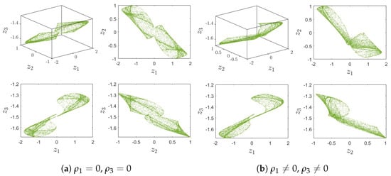
Figure 1. (a) Symmetry for ${\rho }_2=1.78$, $\sigma =0.5$, ${\rho }_4=1$, and ${\rho }_5=-1$. (b) Asymmetry for ${\rho }_1=0.1$, ${\rho }_3=0.1$, ${\rho }_2=1.78$, $\sigma =0.5$, ${\rho }_4=1$, and ${\rho }_5=-1$.

Subsequently, the following theorem is introduced for the discrete system with fractional orders to find the numerical formula.

Theorem 1

([25]). The solution of the fractional difference problem

$$\left\{\begin{array}{c}{}^c\Delta _{\alpha }^{\omega }\chi \left(m\right)=f(m+\omega -1,\chi (m-1+\omega )),\hfill \\ {\Delta }^{\kappa }\chi \left(\alpha \right)={\chi }_{\kappa },r=\lceil \omega \rceil +1\hfill \end{array}\right.$$

(5)

can be indicated as

$$\chi \left(m\right)={\chi }_0\left(\alpha \right)+{\displaystyle \frac{1}{\Gamma \left(\omega \right)}}\sum _{\nu =\alpha +r-\omega }^{m-\gamma }{(m-\nu +1)}^{(\omega -1)}f(\omega -1+\nu ,\chi (\omega -1+\nu )),$$

(6)

where

$${\chi }_0\left(\alpha \right)=\sum _{\kappa =0}^{r-1}{\displaystyle \frac{{(m-\alpha )}^{\kappa }}{\Gamma (\kappa +1)}}{\Delta }^{\kappa }\chi \left(\alpha \right).$$

3. Dynamical Properties of Commensurate Map

The emphasis of this section is on the chaotic behavior of the fractional multi-sigmoidal map (1) with commensurate order.

3.1. Chaotic Analysis

In this subsection, the influence of system factors and fractional order on the dynamics of the map (1) are outlined extensively. The following description of Theorem 1 serves as the basis for the numerical formula of (1) as follows:

$$\left\{\begin{array}{c}{z}_1\left(m\right)=z_1\left(0\right)+{\displaystyle \frac{1}{\Gamma \left(\omega \right)}}{\displaystyle \sum _{\mathsf{ȷ}=0}^m}{\displaystyle \frac{\Gamma (m-1+\omega -\mathsf{ȷ})}{\Gamma (m-\mathsf{ȷ})}}\left({\displaystyle \frac{{\rho }_1}{1+e^{-\sigma z_1(\mathsf{ȷ})}}}+{\rho }_2{z}_1(\mathsf{ȷ})({\left(z_2(\mathsf{ȷ})\right)}^2-1)+{\displaystyle \frac{{\rho }_3}{1+e^{-\sigma z_3(\mathsf{ȷ})}}}-z_1(\mathsf{ȷ})\right),\hfill \\ z_2\left(m\right)=z_2\left(0\right)+{\displaystyle \frac{1}{\Gamma \left(\omega \right)}}{\displaystyle \sum _{\mathsf{ȷ}=0}^m}{\displaystyle \frac{\Gamma (m-1+\omega -\mathsf{ȷ})}{\Gamma (m-\mathsf{ȷ})}}\left(z_1(\mathsf{ȷ})\right),\hfill \\ z_3\left(m\right)=z_3\left(0\right)+{\displaystyle \frac{1}{\Gamma \left(\omega \right)}}{\displaystyle \sum _{\mathsf{ȷ}=0}^m}{\displaystyle \frac{\Gamma (m-1+\omega -\mathsf{ȷ})}{\Gamma (m-\mathsf{ȷ})}}\left({\rho }_{4}sin\left(z_3(\mathsf{ȷ})\right)+{\displaystyle \frac{{\rho }_5}{1+e^{-\sigma z_1(\mathsf{ȷ})}}}-z_3(\mathsf{ȷ})\right).m=1, 2, 3,\cdots \hfill \end{array}\right.$$

(7)

Now, let us use the Jacobian matrix approach to determine the maximum Lyapunov exponents $L{E}_m$ [26] to understand the dynamics of the chaotic area in the fractional map. The tangent map $J_b$ is defined by

$$J_b=\left(\begin{array}{ccc}{S}_1\left(b\right)& S_2\left(b\right)& S_3\left(b\right)\\ R_1\left(b\right)& R_2\left(b\right)& R_3\left(b\right)\\ Q_1\left(b\right)& Q_2\left(b\right)& Q_3\left(b\right)\end{array}\right),$$

(8)

where

$$\left\{\begin{array}{cc}{S}_i\left(b\right)=\hfill & S_i\left(0\right)+{\displaystyle \frac{1}{\Gamma \left(\omega \right)}}{\displaystyle \sum _{\mathsf{ȷ}=0}^{b-1}}{\displaystyle \frac{\Gamma (\omega +b-\mathsf{ȷ}-1)}{\Gamma (b-\mathsf{ȷ})}}({\displaystyle \frac{\sigma {\rho }_1{e}^{-\sigma z_1(\mathsf{ȷ})}}{{(1+e^{-\sigma z_1(\mathsf{ȷ})})}^2}}{S}_i(\mathsf{ȷ})+{\rho }_2({\left(z_2(\mathsf{ȷ})\right)}^2-1)S_i(\mathsf{ȷ})+\hfill \\ \hfill & 2z_2(\mathsf{ȷ}){\rho }_2{z}_1(\mathsf{ȷ})P_i(\mathsf{ȷ})+{\displaystyle \frac{\sigma {\rho }_3{e}^{-\sigma z_3(\mathsf{ȷ})}}{{(1+e^{-\sigma z_3(\mathsf{ȷ})})}^2}}{Q}_i(\mathsf{ȷ})-S_i(\mathsf{ȷ})),\hfill \\ R_i\left(b\right)=\hfill & R_i\left(0\right)+{\displaystyle \frac{1}{\Gamma \left(\omega \right)}}{\displaystyle \sum _{\mathsf{ȷ}=0}^{b-1}}{\displaystyle \frac{\Gamma (\omega +b-\mathsf{ȷ}-1)}{\Gamma (b-\mathsf{ȷ})}}\left(S_i(\mathsf{ȷ})\right),i=1, 2, 3,\hfill \\ Q_i\left(b\right)=\hfill & Q_i\left(0\right)+{\displaystyle \frac{1}{\Gamma \left(\omega \right)}}{\displaystyle \sum _{\mathsf{ȷ}=0}^{b-1}}{\displaystyle \frac{\Gamma (\omega +b-\mathsf{ȷ}-1)}{\Gamma (b-\mathsf{ȷ})}}\left({\rho }_{4}cos\left(z_3(\mathsf{ȷ})\right)Q_i(\mathsf{ȷ})+{\displaystyle \frac{\sigma {\rho }_5{e}^{-\sigma z_1(\mathsf{ȷ})}}{{(1+e^{-\sigma z_1(\mathsf{ȷ})})}^2}}{S}_i(\mathsf{ȷ})-Q_i(\mathsf{ȷ})\right),\hfill \end{array}\right.$$

(9)

Then, $L{E}_{\alpha }$ can be given by

$$L{E}_{\alpha }=\underset{b\to \infty }{lim}{\displaystyle \frac{1}{b}}ln\left|{\lambda }_{\alpha }^{\left(b\right)}\right|,\mathrm{for}\alpha =1,2,3,$$

(10)

where ${\lambda }_{\alpha }^{\left(b\right)}$ are the eigenvalues of $J_b$.

Assign ${\rho }_1=0.1$, ${\rho }_2=1.78,$${\rho }_3=0.1,$$\sigma =0.5$, ${\rho }_4=-1,$${\rho }_5=1$, and $(z_1\left(0\right),z_2\left(0\right),z_3\left(0\right))=(0.06,0.06,-0.3)$ (IC). We experiment with commensurate orders $\omega$, like expanding the chaotic area, to gain a better understanding of how commensurate orders affect the behaviors of the novel fractional multi-sigmoidal map (1). We plot bifurcation charts and related plots $L{E}_m$ in Figure 2 with relation to $\omega \in [0.7,1]$, where the $LEm$ are positive; we can observe that the states turn completely chaotic.

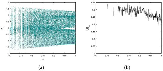
Figure 2. (a) Bifurcation of (1) for $\omega \in [0.7,1]$. (b) The corresponding $LEm$.

Figure 3 displays the bifurcation charts for the $\omega =0.92$ order. Specifically, when ${\rho }_1$ and ${\rho }_3$ are in $[0,0.3]$, the states of the map (1) are shown to be completely chaotic. Moreover, the behaviors of the map transition from stable to period-doubling bifurcation when ${\rho }_2$ is within $[1.5,1.9]$. The trajectories are periodic windows with four-period orbits when ${\rho }_2$ is within $[1.5,1.625]$, whereas the system becomes a period-doubling bifurcation when $1.625<{\rho }_2<1.88$. Furthermore, when ${\rho }_2$ increases, the model exhibits a divergence toward infinity. Additionally, when ${\rho }_4$ is within $[-3,3]$, the trajectories of the system become chaotic. We can observe that when ${\rho }_4$ in $[-3,-1]$, the map indicates period-doubling bifurcation. It is apparent that the behaviors of a novel fractional multi-sigmoidal map (1) are affected by all aspects of the model and changes in the commensurate derivative $\omega$ affect the rich behaviors of a commensurate multiple sigmoidal map (1). It suggests that the bifurcation point is influenced by the order in this instance. It is also possible to see the usual symmetry-breaking bifurcation.

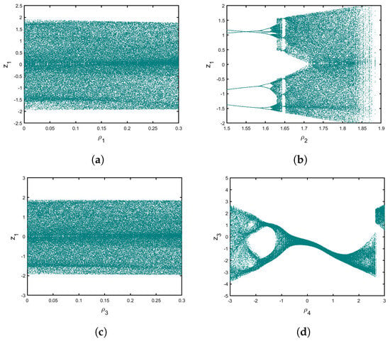
Figure 3. Bifurcation of (1) for $\omega =0.95$ versus (a) ${\rho }_1\in [0,0.3]$, (b) ${\rho }_2\in [1.5,1.9]$, (c) ${\rho }_3\in [0,0.3]$, and (d) ${\rho }_4\in [-3,3]$.

For completeness, the commensurate multiple sigmoidal map’s evolution states for $\omega =0.92$ are depicted in Figure 4. Furthermore, the asymmetry chaotic attractors without fixed points for different commensurate orders $\omega$ are revealed, as illustrated in Figure 5, indicating that the symmetric-breaking attractor remains unaffected by the increase in order. Consequently, these results indicate that the structure of the hidden attractors of the fractional system is established by commensurate orders (1).

Figure 4. Numerical evolution of the commensurate multi-sigmoidal map (1) for $\omega =0.92$.

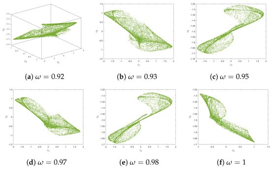
Figure 5. Hidden asymmetry attractors of (1) for various $\omega$ orders.

3.2. Entropy Test

The complexity of the novel commensurate multi-sigmoidal map (1) is statistical using the approximate entropy algorithm [27], where higher $ApEn$ indicates more chaotic behavior. The $ApEn$ algorithm is defined theoretically as follows for $t=0.2std\left(Z\right)$ and the embedding dimension $m=2$:

$$ApEn={\mathrm{Y}}^m\left(t\right)-{\mathrm{Y}}^{m+1}\left(t\right),$$

(11)

where ${\mathrm{Y}}^m\left(t\right)$ is identified as

$${\mathrm{Y}}^m\left(t\right)={\displaystyle \frac{1}{n-m+1}}\sum _{\iota =1}^{n-m+1}log{C}_{\iota }^m\left(t\right).$$

(12)

Table 1 displays the $ApEn$ calculation of the commensurate multi-sigmoidal map (1) for a range of $\omega$ values of fractional commensurate order. It is clear that for $\omega =0.92,0.95$, higher values in the ApEn results signify a higher degree of map complexity, while Figure 6 illustrates the $ApEn$ plots for versus the $\omega \in [0.7,1]$ order with the ${\rho }_2\in [1.5,1.9]$ parameter, the highest $ApEn$ values are obtained when the fractional map is chaotic. Therefore, this result validates the occurrence of chaos in the fractional multi-sigmoidal map (1) and agrees with the previous findings.

Table 1. ApEn of (1) for different commensurate fractional orders $\omega$.

${\mathit{\omega }}_1$	${\mathit{\omega }}_2$	${\mathit{\omega }}_3$	$\mathit{ApEn}$
0.92	0.92	0.92	0.4103
0.95	0.95	0.95	0.4583
0.9	0.9	0.9	0.2629
1	1	1	0.3885

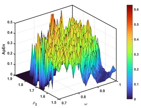
Figure 6. The $ApEn$ of commensurate map (1) depends on the system parameter ${\rho }_2$ and the fractional order $\omega$.

4. Dynamical Properties of Incommensurate Map

Here, we utilize bifurcation and the associated $\left(L{E}_m\right)$ to look into the effects of the incommensurate fractional values $({\omega }_1,{\omega }_2,{\omega }_3)$ and the system factors on the dynamics of the suggested novel multi-sigmoidal map. The incommensurate order formula of the multiple sigmoidal map is displayed as follows:

$$\left\{\begin{array}{cc}\hfill {}^c\Delta _{\alpha }^{{\omega }_1}{z}_1\left(m\right)& ={\displaystyle \frac{{\rho }_1}{1+e^{-\sigma z_1\left({\vartheta }_1\right)}}}+{\rho }_2{z}_1\left({\vartheta }_1\right)({\left(z_2\left({\vartheta }_1\right)\right)}^2-1)+\hfill \\ \hfill & {\displaystyle \frac{{\rho }_3}{1+e^{-\sigma z_3\left({\vartheta }_1\right)}}}-z_1\left({\vartheta }_1\right),\hfill \\ \hfill {}^c\Delta _{\alpha }^{{\omega }_2}{z}_2\left(m\right)& =z_1\left({\vartheta }_2\right),\hfill \\ \hfill {}^c\Delta _{\alpha }^{{\omega }_3}{z}_3\left(m\right)& ={\rho }_{4}sin\left(z_3\left({\vartheta }_3\right)\right)+{\displaystyle \frac{{\rho }_5}{1+e^{-\sigma z_1\left({\vartheta }_3\right)}}}-z_3\left({\vartheta }_3\right),\hfill \end{array}\right.$$

(13)

where ${\vartheta }_1=m-1+{\omega }_1$, ${\vartheta }_2=m-1+{\omega }_2$, and ${\vartheta }_3=m-1+{\omega }_3$.

4.1. Chaotic Dynamics

In this subsection, we represent the numerical formula of (13) as follows:

$$\left\{\begin{array}{c}{z}_1\left(m\right)=z_1\left(0\right)+{\displaystyle \frac{1}{\Gamma \left({\omega }_1\right)}}{\displaystyle \sum _{\mathsf{ȷ}=0}^m}{\displaystyle \frac{\Gamma (m-1+{\omega }_1-\mathsf{ȷ})}{\Gamma (m-\mathsf{ȷ})}}\left({\displaystyle \frac{{\rho }_1}{1+e^{-\sigma z_1(\mathsf{ȷ})}}}+{\rho }_2{z}_1(\mathsf{ȷ})({\left(z_2(\mathsf{ȷ})\right)}^2-1)+{\displaystyle \frac{{\rho }_3}{1+e^{-\sigma z_3(\mathsf{ȷ})}}}-z_1(\mathsf{ȷ})\right),\hfill \\ z_2\left(m\right)=z_2\left(0\right)+{\displaystyle \frac{1}{\Gamma \left({\omega }_2\right)}}{\displaystyle \sum _{\mathsf{ȷ}=0}^m}{\displaystyle \frac{\Gamma (m-1+{\omega }_2-\mathsf{ȷ})}{\Gamma (m-\mathsf{ȷ})}}\left(z_1(\mathsf{ȷ})\right),\hfill \\ z_3\left(m\right)=z_3\left(0\right)+{\displaystyle \frac{1}{\Gamma \left({\omega }_3\right)}}{\displaystyle \sum _{\mathsf{ȷ}=0}^m}{\displaystyle \frac{\Gamma (m-1+{\omega }_3-\mathsf{ȷ})}{\Gamma (m-\mathsf{ȷ})}}\left({\rho }_{4}sin\left(z_3(\mathsf{ȷ})\right)+{\displaystyle \frac{{\rho }_5}{1+e^{-\sigma z_1(\mathsf{ȷ})}}}-z_3(\mathsf{ȷ})\right).m=1, 2, 3,\cdots \hfill \end{array}\right.$$

(14)

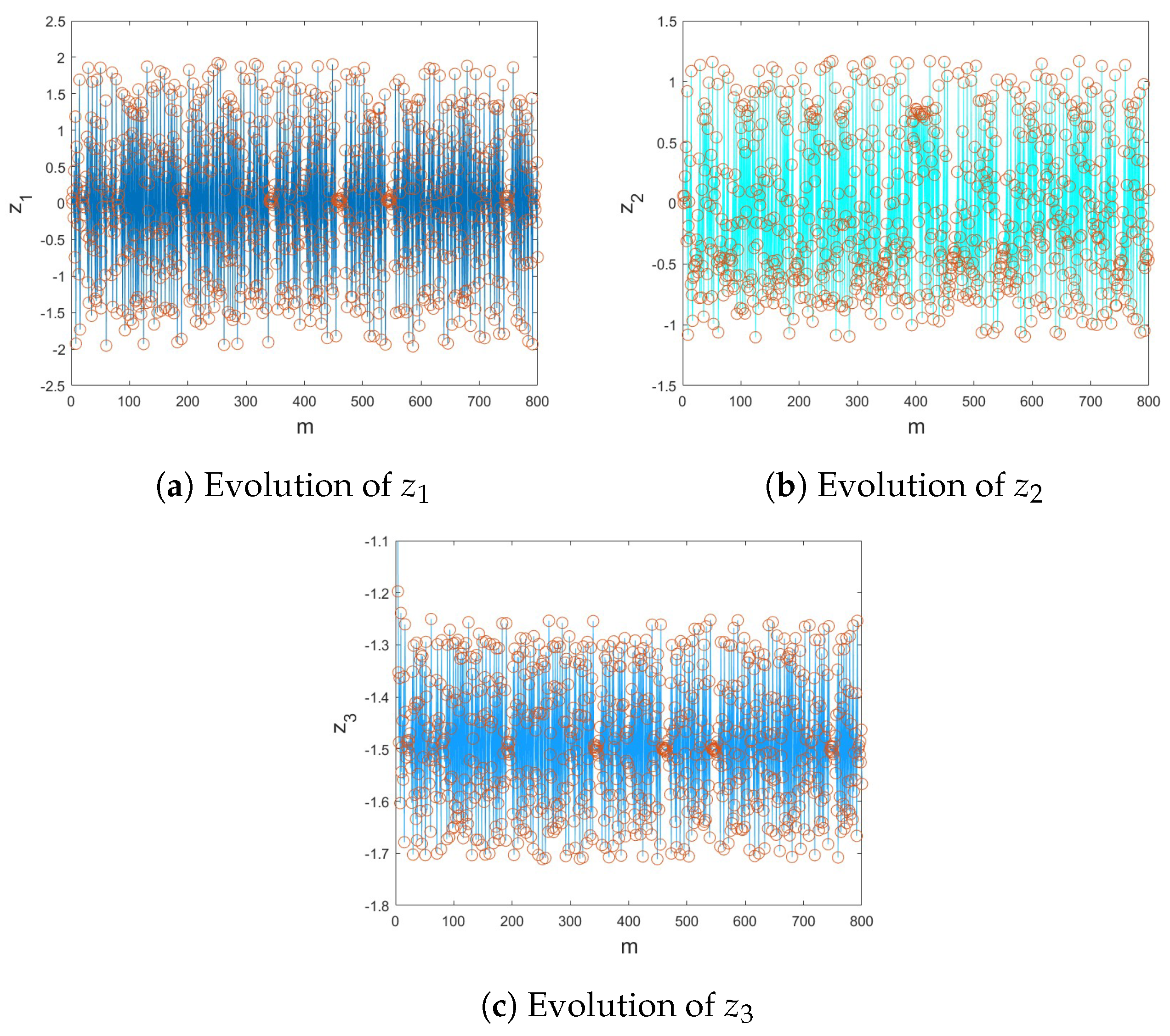
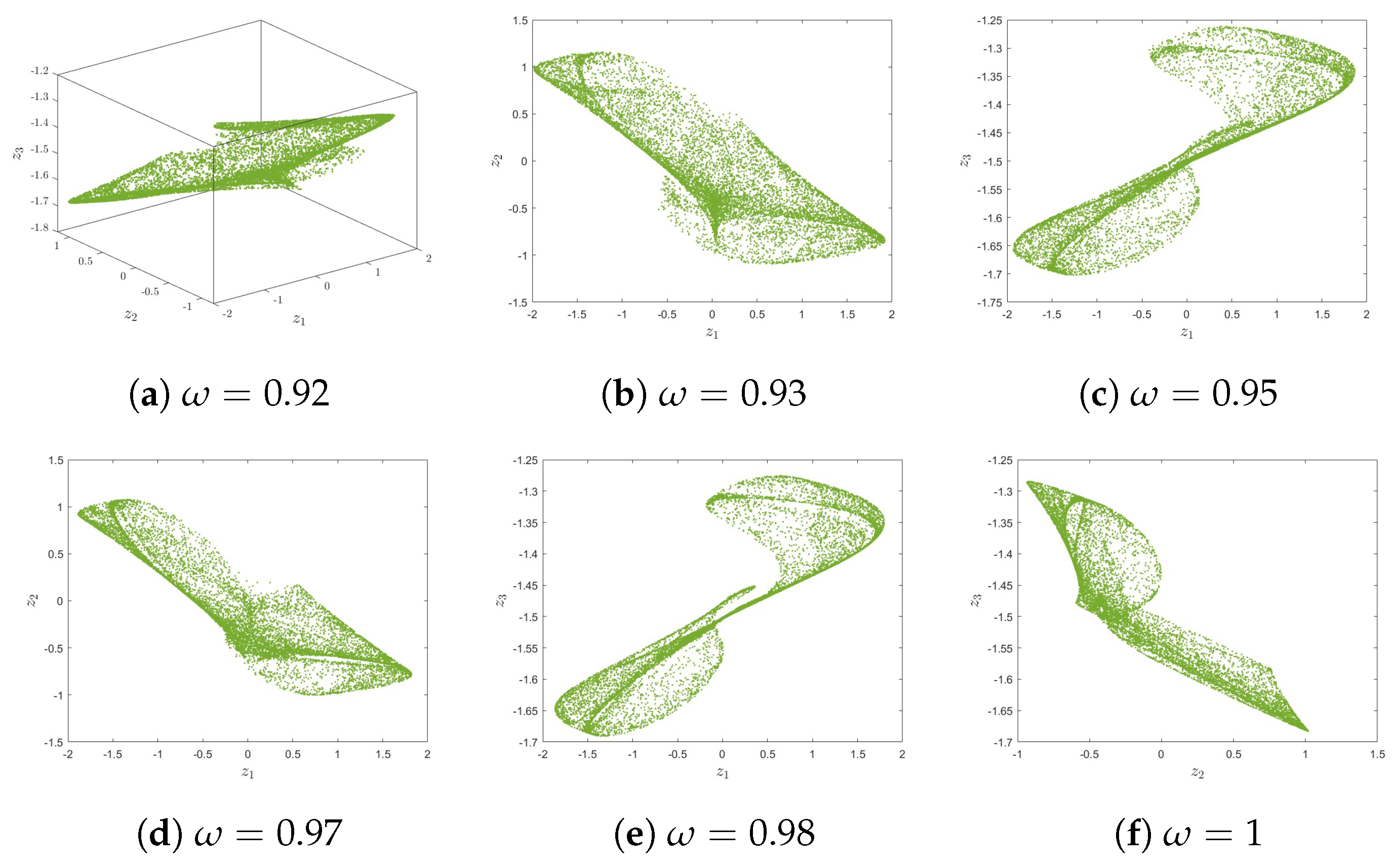
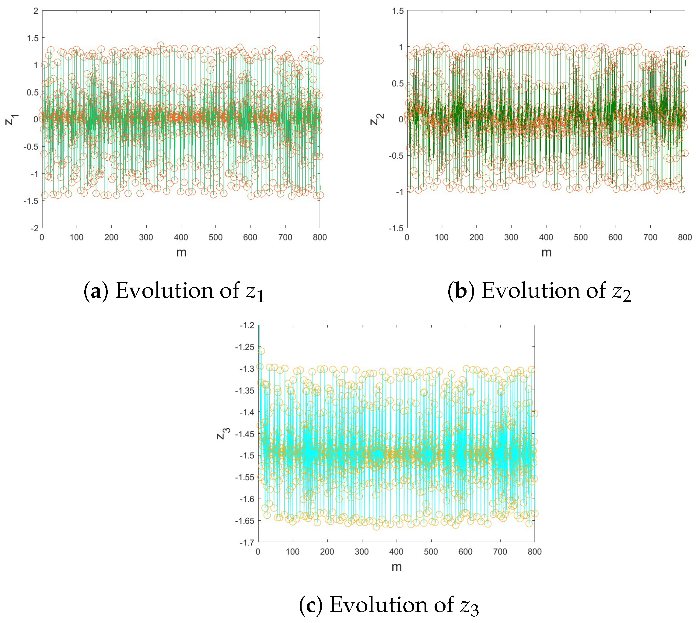
Initially, the numerical simulations for the suggested incommensurate-order multi-sigmoidal map (13) are represented in Figure 7 when $({\omega }_1,{\omega }_2,{\omega }_3)=(1,0.5,0.85)$, and the hidden attractors are depicted by various incommensurate orders $({\omega }_1,{\omega }_2,{\omega }_3)$ with IC in Figure 8.

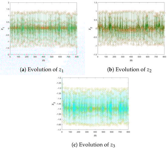
Figure 7. Numerical evolution of the incommensurate multi-sigmoidal map (13) for $({\omega }_1,{\omega }_2,{\omega }_3)=(1,0.5,0.85)$.

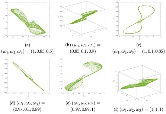
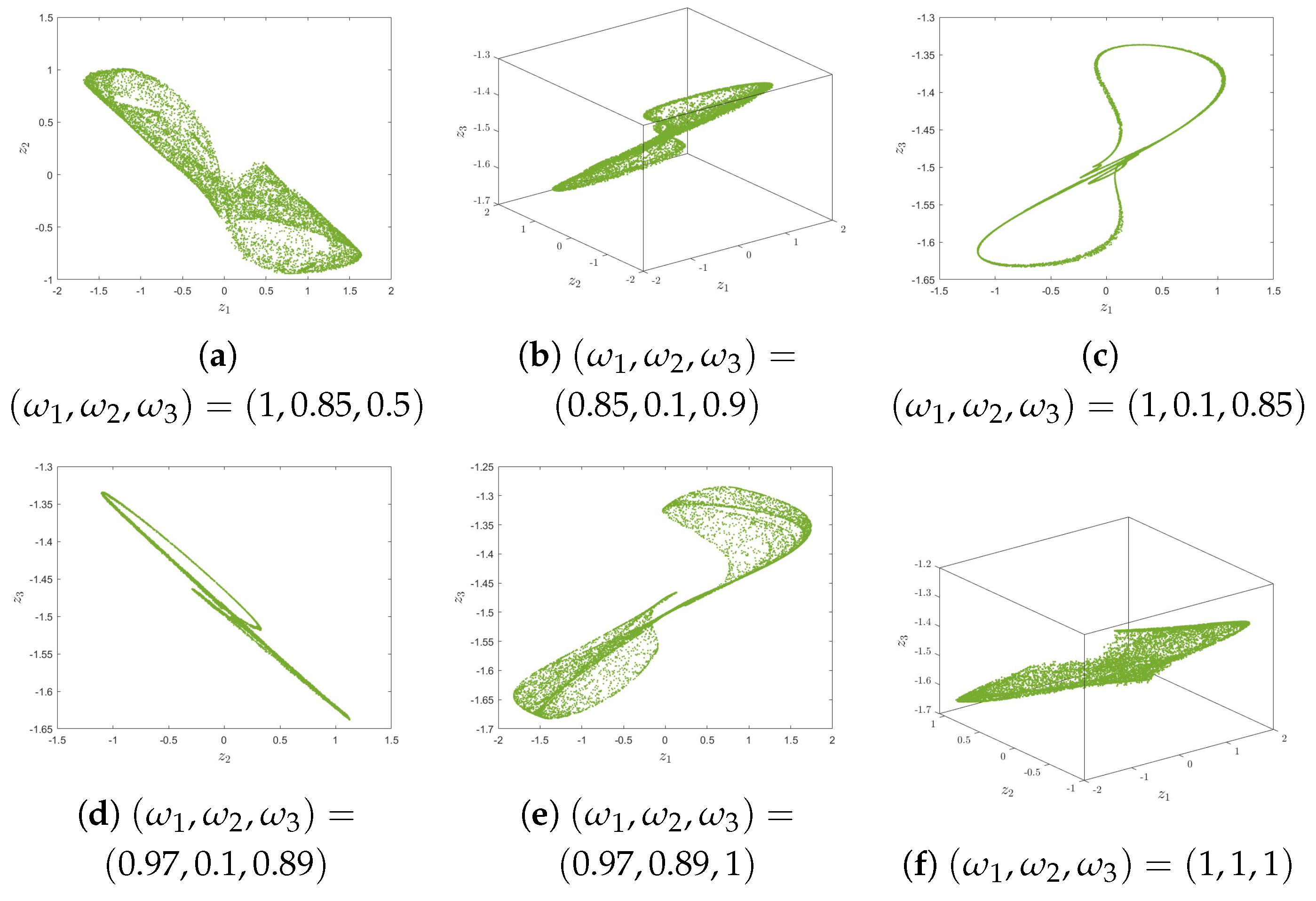
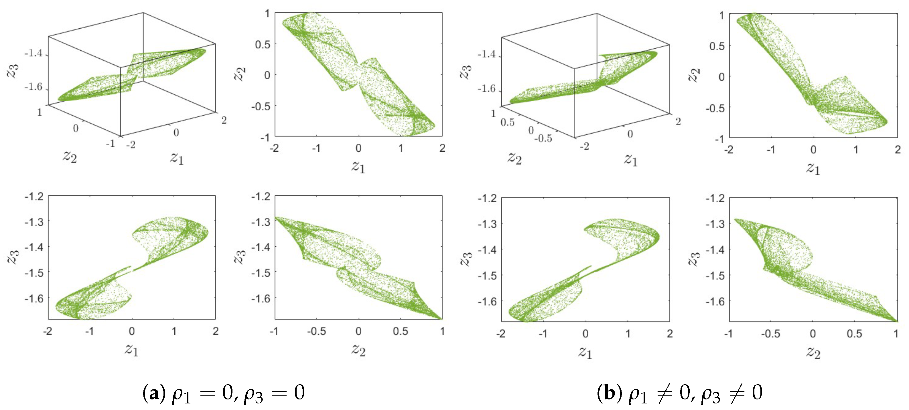
Figure 8. Hidden asymmetry phases of (13) for various values of $({\omega }_1,{\omega }_2,{\omega }_3)$.

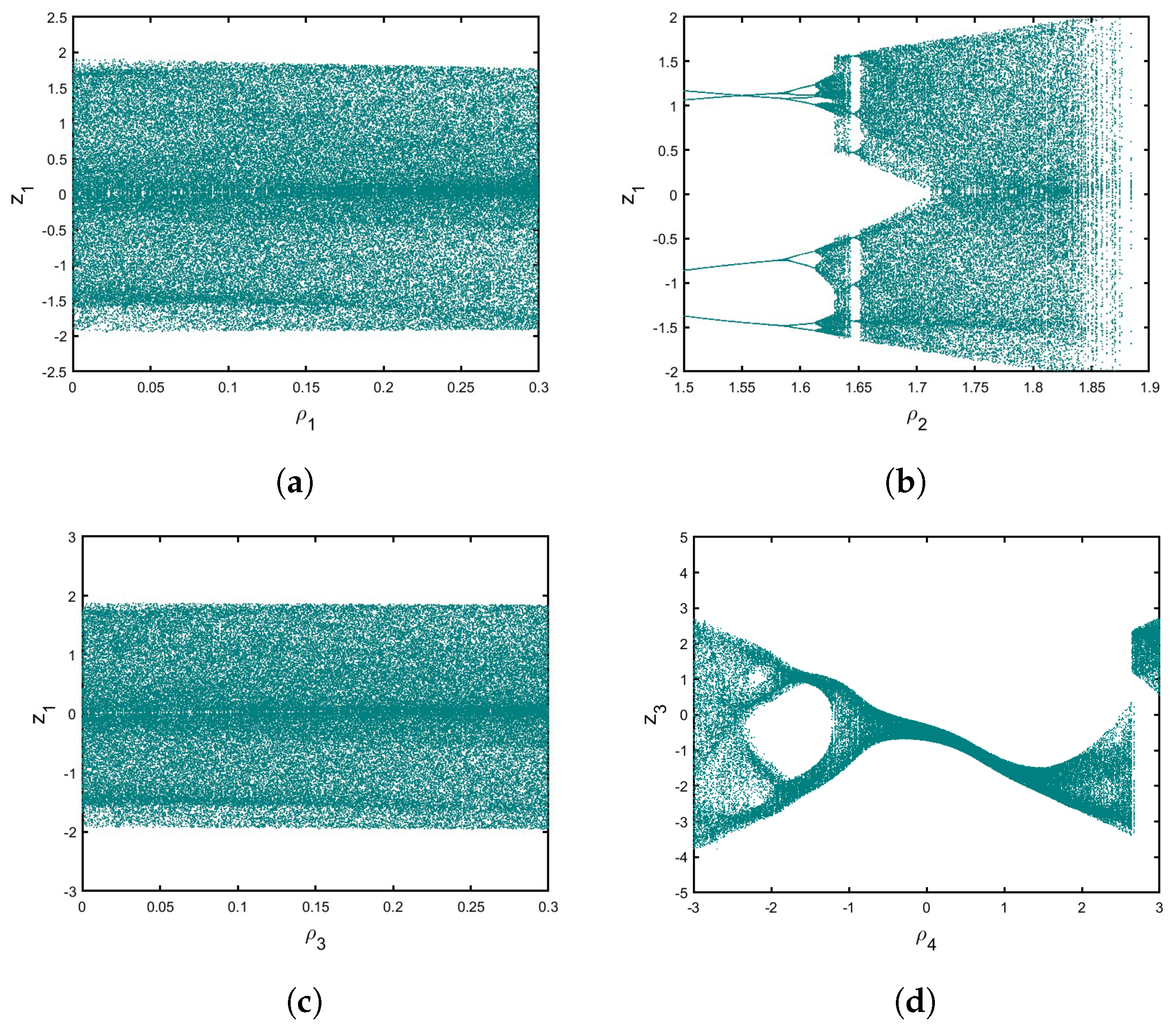
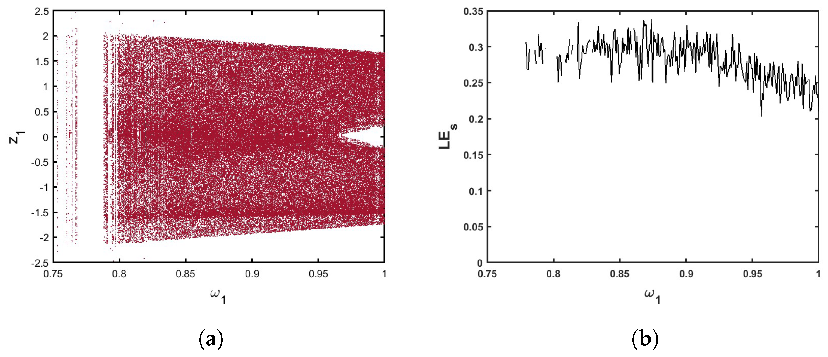
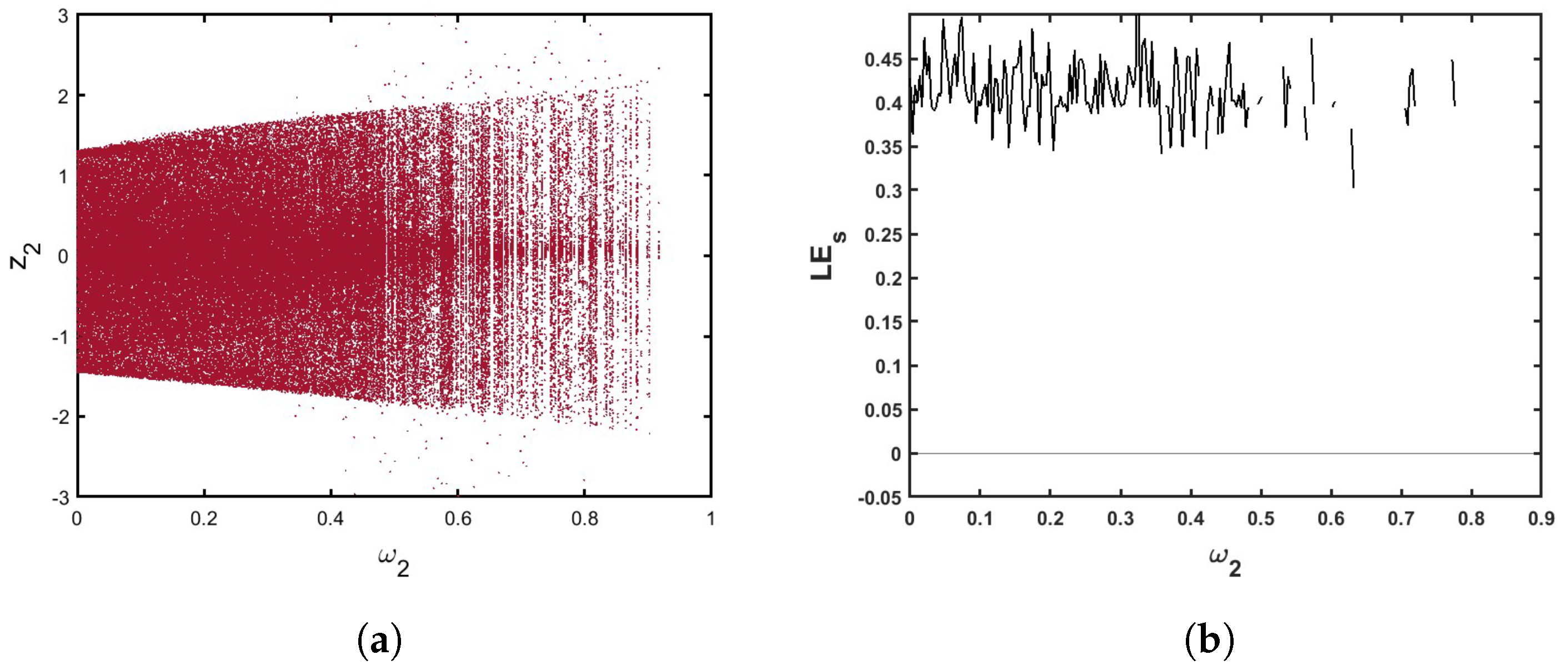
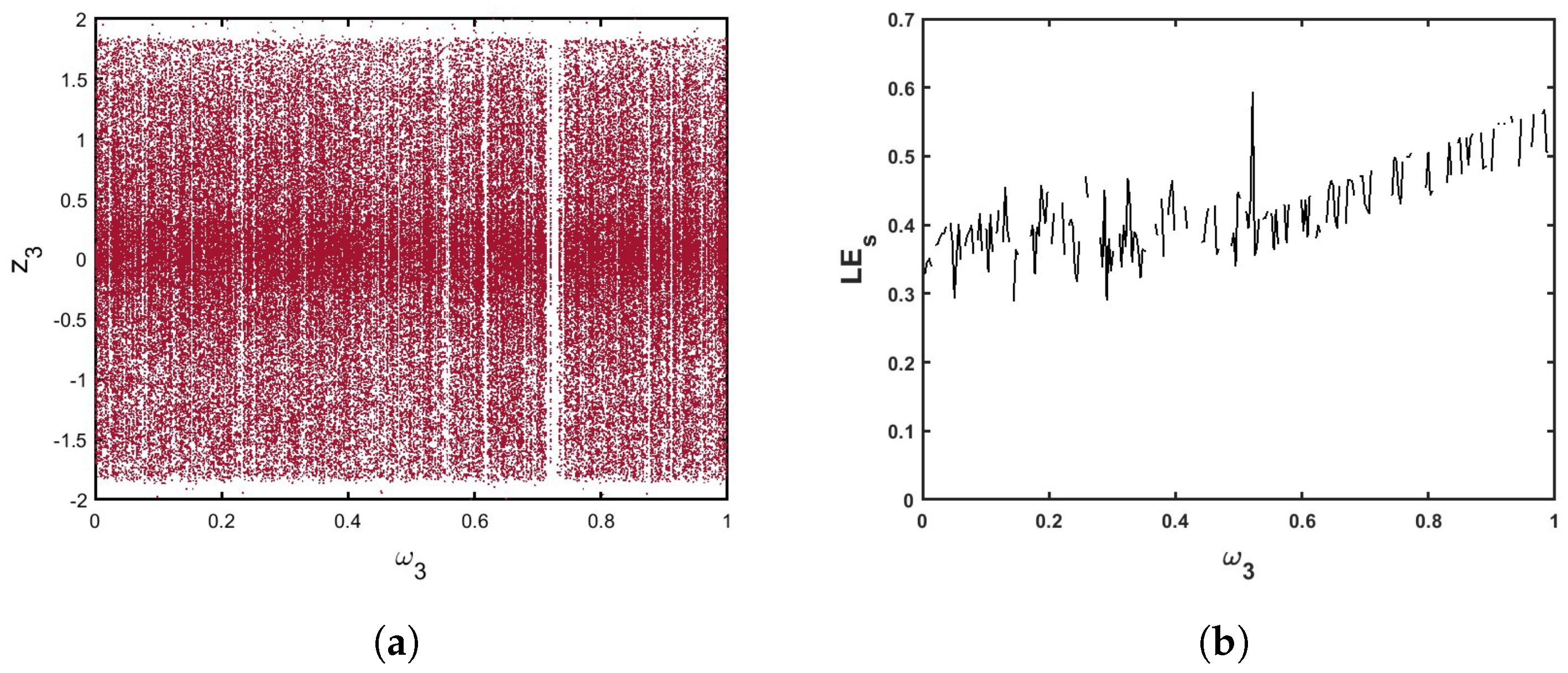
In order to investigate the effects of incommensurate orders on the behaviors of the map (13), as an illustration to the incommensurate order values ${\omega }_1$, ${\omega }_2$, and ${\omega }_3$, we produced a diagram of the bifurcation and the related plots $LEm$. When we choose ${\omega }_2=0.5$, ${\omega }_3=0.85$, and ${\omega }_1\in [0.75,1]$ in Figure 9, the trajectories manifest a divergence toward infinity in $[0.75,0.87]$, and their $LEm$ values are positive in ${\omega }_1\in [0.88,1]$, where they become chaotic. Additionally, in Figure 10 with ${\omega }_2\in (0,1]$ and fixed ${\omega }_1=0.85$ and ${\omega }_3=0.5$, observably, the states of the map are totally chaotic in $[0,0.5]$ and divergence toward infinity when ${\omega }_2$ gristly increases until it approaches unity. Furthermore, in Figure 11, we fixed ${\omega }_1=0.85$, ${\omega }_2=0.5$ and versus ${\omega }_3$ between $0.4$ and 1 to show the dynamics trajectories of the proposed multi-sigmoidal-based memristive map (13). When ${\omega }_3\in [0.4,0.58]\cup [0.68,1]$, it is observed that $LEm$ gradually increases, which indicates the existence of chaos and divergence toward infinity when ${\omega }_3\in [0.59,0.67]$. Thus, a new fractional multiple sigmoidal map (13) exhibits complex behaviors that are affected by variations in the incommensurate orders.

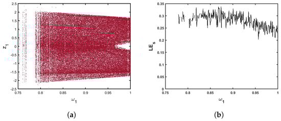
Figure 9. (a) Bifurcation of (13) for ${\omega }_1\in [0.75,1]$ and ${\omega }_2=0.5$, ${\omega }_2=0.85$. (b) The corresponding $LEm$.

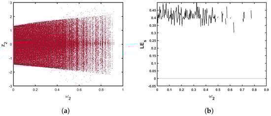
Figure 10. (a) Bifurcation of (13) for ${\omega }_2\in (0,1]$ and ${\omega }_1=0.85$, ${\omega }_3=0.5$. (b) The corresponding $LEm$.

Figure 11. (a) Bifurcation of (13) for ${\omega }_3\in (0,1]$ and ${\omega }_1=0.85$, ${\omega }_2=0.5$. (b) The corresponding $LEm$.

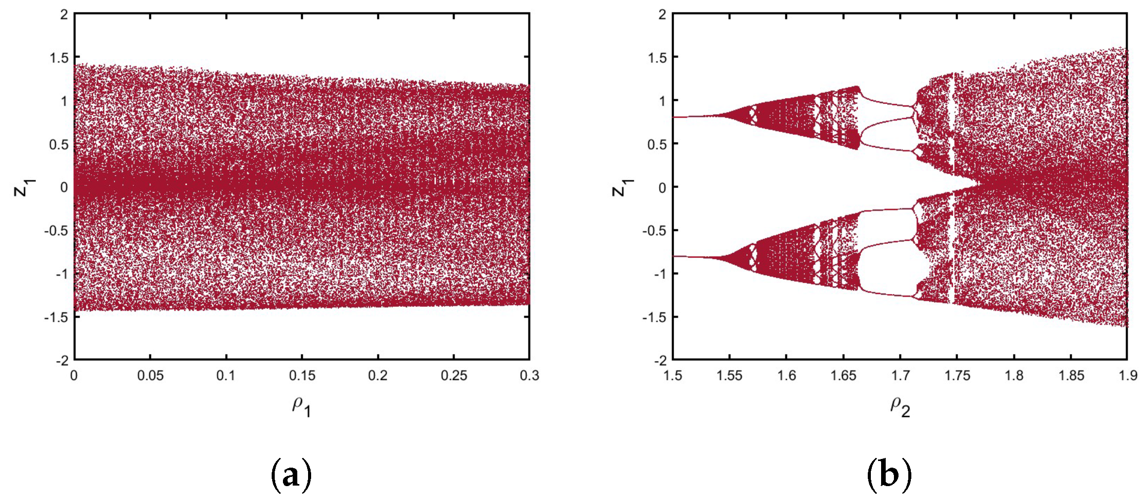
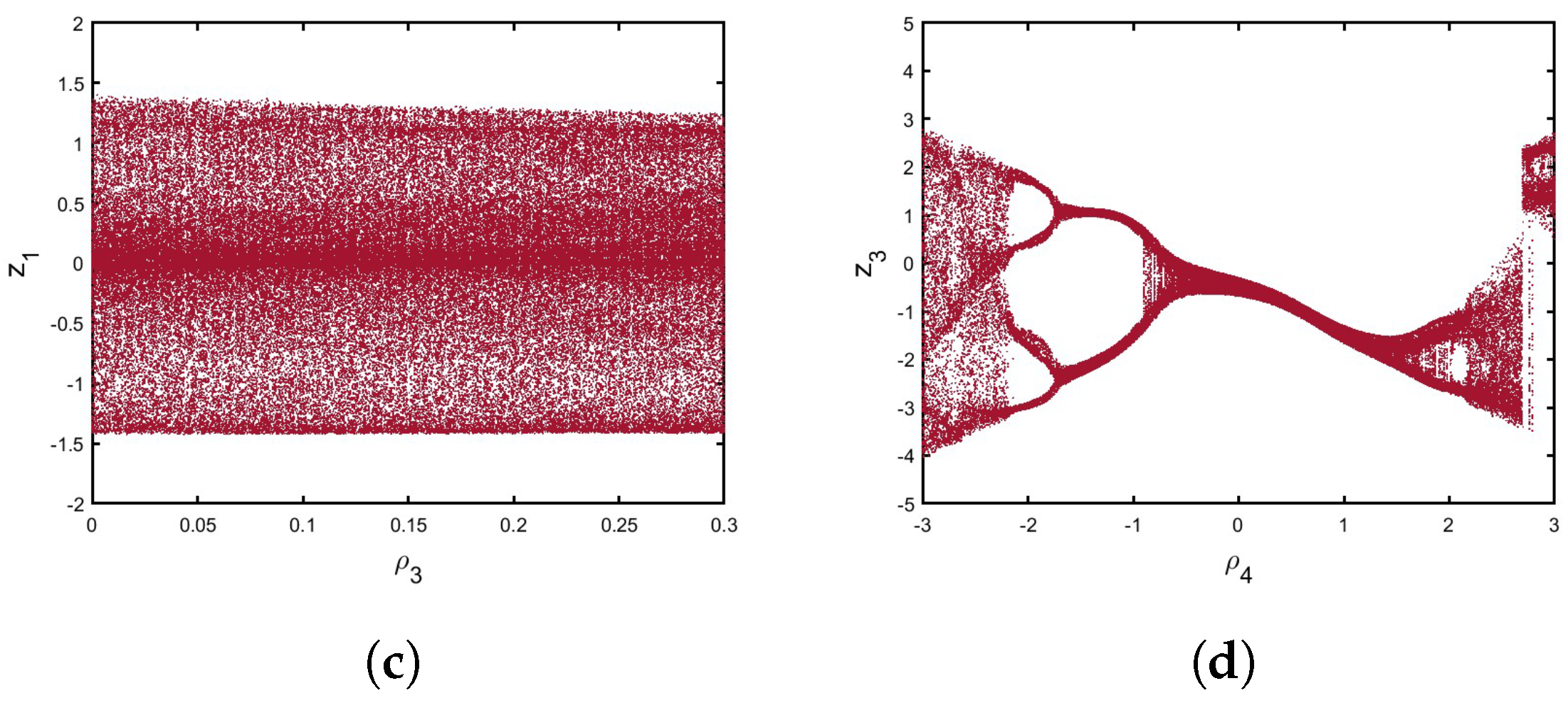
Additionally, Figure 12 displays the bifurcation charts for $({\omega }_1,{\omega }_2,{\omega }_3)=(1,0.5,0.85)$ when ${\rho }_1$ and ${\rho }_3$ versus in $[0,0.3]$; obviously, the states of the incommensurate multi-sigmoidal map (13) are totally chaotic. The dynamics shift from periodic to period-doubling bifurcation when ${\rho }_2$ is in $[1.5,1.9]$. Trajectories are periodic when ${\rho }_2$ is at $[1.5,1.55]$, but the map exhibits chaotic behavior when ${\rho }_2\in [1.55,1.66]$. Moreover, when $1.72<{\rho }_2<1.9$, the map becomes a period-doubling bifurcation, and the states in $[1.67,1.72]$ are periodic windows with six-period orbits. Furthermore, when ${\rho }_4$ is in $[-3,3]$, the trajectories of the map become chaotic. We can see that with ${\rho }_4$ in $[-3,-1]$, the map indicates period-doubling bifurcation. This implies that the order affects the bifurcation point. In addition, typical symmetry-breaking bifurcation can be observed. Thus, the behaviors of a novel incommensurate fractional multi-sigmoidal map (13) are impacted by the factors of the system, and varied incommensurate orders affect the dynamics of the incommensurate multiple sigmoidal map (13). As a result, the findings show that the order is a crucial bifurcation parameter that influences the map’s dynamics.

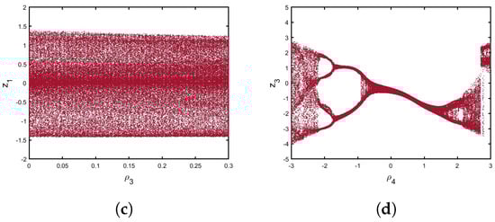
Figure 12. Bifurcation of (13) for $({\omega }_1,{\omega }_2,{\omega }_3)=(1,0.5,0.85)$ versus (a) ${\rho }_1\in [0,0.3]$, (b) ${\rho }_2\in [1.5,1.9]$, (c) ${\rho }_3\in [0,0.3]$, and (d) ${\rho }_4\in [-3,3]$.

4.2. $C_0$ Complexity

This part uses the $C_0$ complexity algorithm [28]. Using the Fourier inverse transform, we determine the $C_0$ complexity of the incommensurate multi-sigmoidal map (13), detailed as follows for $\left\{\varphi \right(\zeta ),\zeta =0,1,\dots ,R-1\}$:

• To determine the Fourier transform of $\varphi \left(\zeta \right)$, we define

  $${\mathbf{Z}}_R\left(\zeta \right)={\displaystyle \frac{1}{R}}\sum _{\zeta =0}^{R-1}\varphi \left(\zeta \right){exp}^{-2\pi i\left({\displaystyle \frac{kj}{R}}\right)},\zeta =0,1,...,R-1.$$

  (15)
• We explain the mean square of ${\mathbf{Z}}_R\left(\zeta \right)$ as $G_R={\displaystyle \frac{1}{R}}{\sum }_{\zeta =0}^{N-1}{\left|{\mathbf{Z}}_R\left(\zeta \right)\right|}^2$ and set

  $${\overline{\mathbf{Z}}}_R\left(\zeta \right)=\left\{\begin{array}{cc}{\mathbf{Z}}_R\left(\zeta \right)\hfill & \mathrm{if}\parallel {\mathbf{Z}}_R{\left(\zeta \right)\parallel }^2>{rG}_R,\hfill \\ 0\hfill & \mathrm{if}\parallel {\mathbf{Z}}_R{\left(\zeta \right)\parallel }^2\le {rG}_R.\hfill \end{array}\right.$$

  (16)
• To determine the inverse Fourier transform, we employ the following formula:

  $$\delta (\mathsf{ȷ})={\displaystyle \frac{1}{R}}\sum _{\zeta =0}^{R-1}{\overline{\mathbf{Z}}}_X\left(\zeta \right){exp}^{2\pi i({\displaystyle \frac{\mathsf{ȷ}\zeta }{R}})},\mathsf{ȷ}=0,1,\dots ,R-1.$$

  (17)
• Utilizing the subsequent formula, the $C_0$ complexity obtained as

  $$C_0={\displaystyle \frac{{\sum }_{\mathsf{ȷ}=0}^{R-1}\parallel \delta (\mathsf{ȷ})-\varphi (\mathsf{ȷ})\parallel }{{\sum }_{\mathsf{ȷ}=0}^{R-1}{\parallel \varphi (\mathsf{ȷ})\parallel }^2}}.$$

  (18)

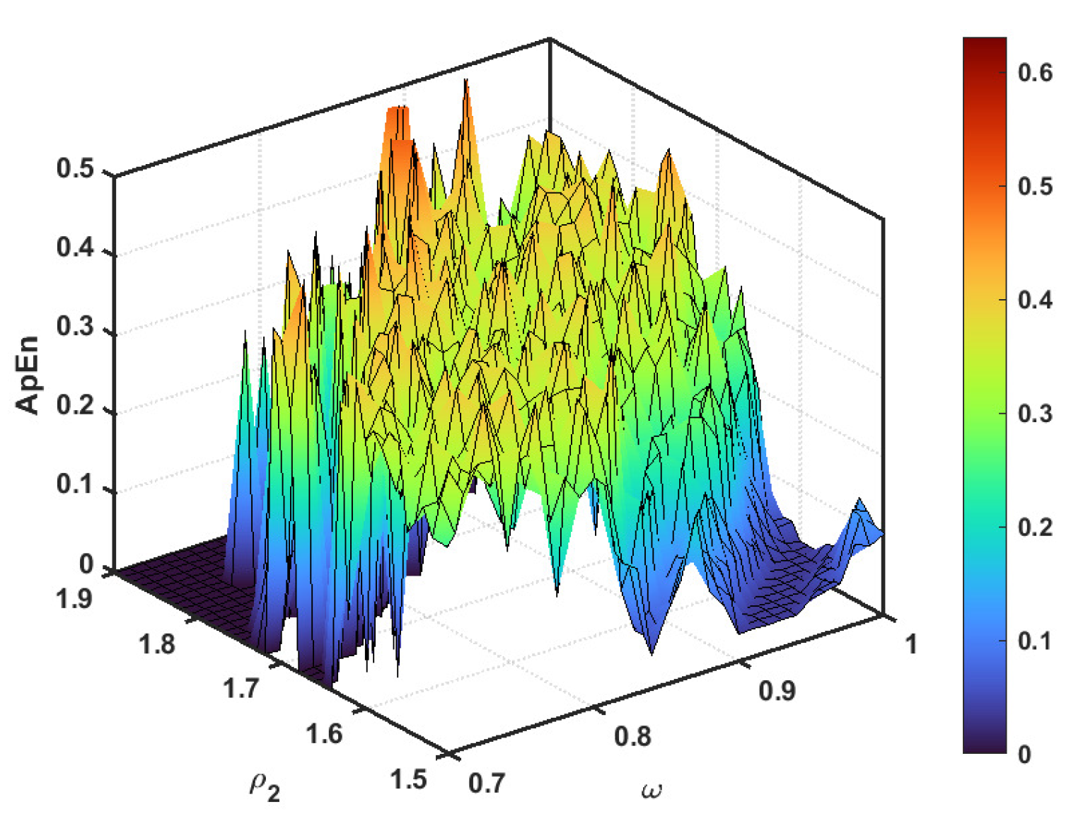
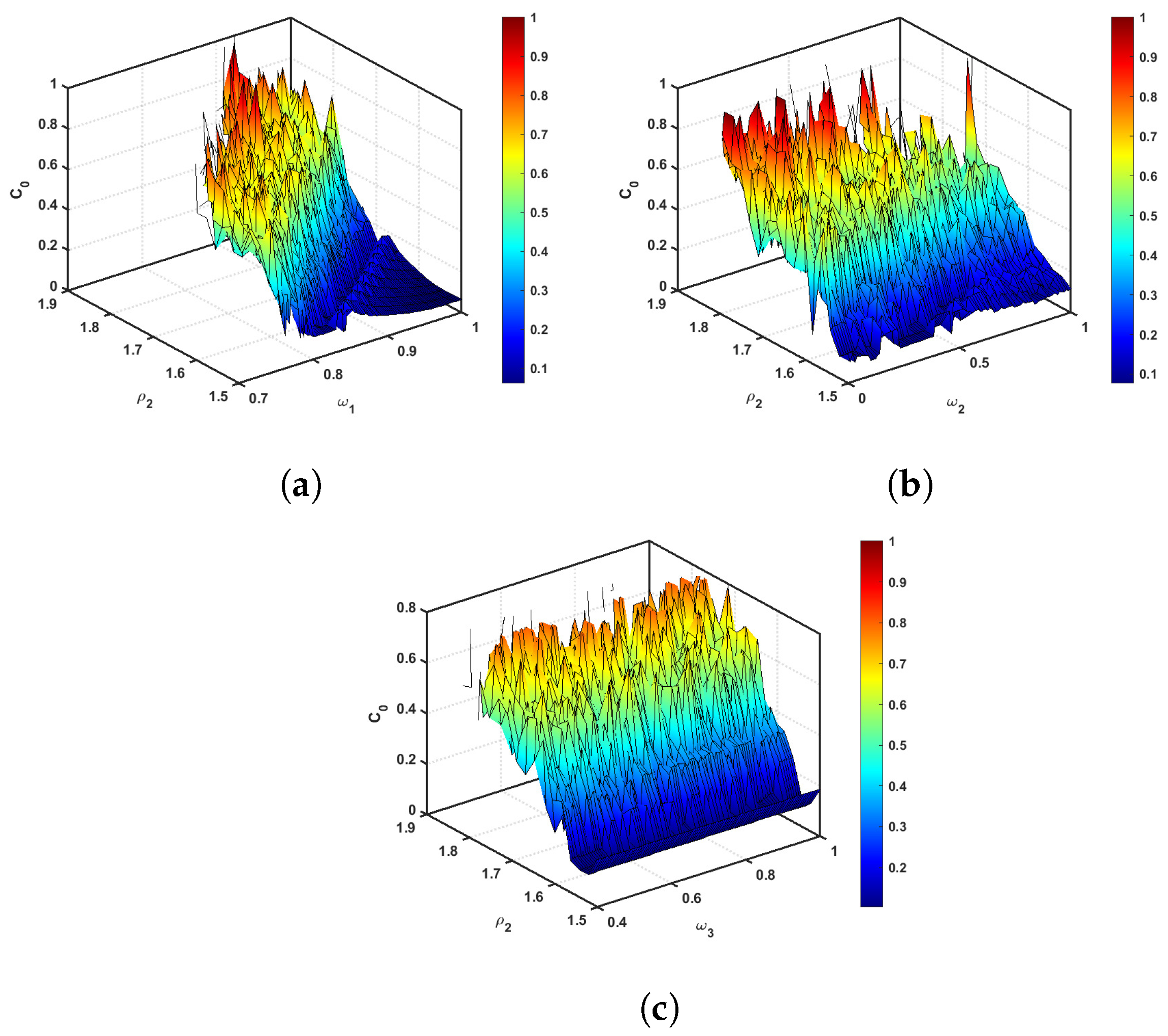
We evaluate the $C_0$ complexity numerically for the incommensurate multi-sigmoidal map (13). The various fractional orders ${\omega }_1$, ${\omega }_2$, and ${\omega }_3$ where ${\rho }_2\in [1.5,1.9]$ change, as shown in Figure 13. As the $C_0$ complexity result increases, the map becomes more complex. The previous results are consistent with these $C_0$ complexity findings.

Figure 13. The $C_0$ complexity of the incommensurate multi-sigmoidal map (13) versus ${\rho }_2\in [1.5,1.9]$ with (a) ${\omega }_1\in [0.75,1]$ for ${\omega }_2=0.5$ and ${\omega }_3=0.85$, (b) ${\omega }_2\in (0,1]$ for ${\omega }_1=0.85$ and ${\omega }_3=0.5$, and (c) ${\omega }_3\in (0,1]$ for ${\omega }_1=0.85$ and ${\omega }_2=0.5$.

5. Control

A control scheme to stabilize the commensurate multi-sigmoidal map (1) and the incommensurate multiple sigmoidal map (13) is shown in this section. This will guarantee that the states of the maps converge to zero in a sufficient amount of time.

5.1. The Commensurate Chaos Control

In this case, we use the following Lemma to develop a nonlinear controller that will stabilize the commensurate multi-sigmoidal map (1) and ensure that each state asymptotically approaches zero:

Lemma 1

([29]). The linear commensurate system is

$${}^C\Delta _{\alpha }^{\omega }\chi \left(m\right)=\mathit{D}\chi (m-1+\omega ).$$

(19)

Let $\chi \left(m\right)={({\chi }_1\left(m\right),...,{\chi }_n\left(m\right))}^T$, $0<\omega \le 1$ and $\forall m\in {\mathbb{N}}_{\alpha +1-\omega }$. Matrix $\mathit{D}\in R^{n\times n}$, possess asymptotically stable zero equilibrium if

$${\lambda }_j\in \left\{\eta \in \mathbb{C}:\left|\eta \right|<{\left(2cos{\displaystyle \frac{\left|arg\eta \right|-\pi }{2-\omega }}\right)}^{\omega }\mathrm{and}\left|arg\eta \right|>{\displaystyle \frac{\omega \pi }{2}}\right\},$$

(20)

for all ${\lambda }_j$ of $\mathit{D}$.

Now, the following describes the 3D controlled map via commensurate order:

$$\left\{\begin{array}{cc}\hfill {}^c\Delta _{\alpha }^{\omega }{z}_1\left(m\right)& ={\displaystyle \frac{{\rho }_1}{1+e^{-\sigma z_1\left(\vartheta \right)}}}+{\rho }_2{z}_1\left(\vartheta \right)({\left(z_2\left(\vartheta \right)\right)}^2-1)+\hfill \\ \hfill & {\displaystyle \frac{{\rho }_3}{1+e^{-\sigma z_3\left(\vartheta \right)}}}-z_1\left(\vartheta \right)+{\mathbf{C}}_1\left(\vartheta \right),\hfill \\ \hfill {}^c\Delta _{\alpha }^{\omega }{z}_2\left(m\right)& =z_1\left(\vartheta \right)+{\mathbf{C}}_2\left(\vartheta \right),\hfill \\ \hfill {}^c\Delta _{\alpha }^{\omega }{z}_3\left(m\right)& ={\rho }_{4}sin\left(z_3\left(\vartheta \right)\right)+{\displaystyle \frac{{\rho }_5}{1+e^{-\sigma z_1\left(\vartheta \right)}}}-z_3\left(\vartheta \right)+{\mathbf{C}}_3\left(\vartheta \right),\hfill \end{array}\right.$$

(21)

Based on Lemma 1, the adaptive controllers ${({\mathbf{C}}_1,{\mathbf{C}}_2,{\mathbf{C}}_3)}^T$ are used to design the adaptive controller for controlling the commensurate multi-sigmoidal map (1).

Proposition 1.

The commensurate map (1) can be stabilized with the 3D control law

$$\left\{\begin{array}{ccc}\hfill {\mathit{C}}_1\left(\vartheta \right)& ={\rho }_2{z}_1\left(\vartheta \right)-{\displaystyle \frac{{\rho }_1}{1+e^{-\sigma z_1\left(\vartheta \right)}}}-{\displaystyle \frac{{\rho }_3}{1+e^{-\sigma z_3\left(\vartheta \right)}}}\hfill & \hfill -{\rho }_2{z}_1\left(\vartheta \right){\left(z_2\left(\vartheta \right)\right)}^2\\ \hfill {\mathit{C}}_2\left(\vartheta \right)& =-{\displaystyle \frac{1}{2}}{z}_2\left(\vartheta \right)\hfill \\ \hfill {\mathit{C}}_3\left(\vartheta \right)& =-{\displaystyle \frac{{\rho }_5}{1+e^{-\sigma z_1\left(\vartheta \right)}}}-{\rho }_{4}sin\left(z_3\left(\vartheta \right)\right).\hfill \end{array}\right.$$

(22)

Proof. 

Substituting (22) into (21), we obtain

$${}^c\Delta _{\alpha }^{\omega }\overline{U}=A\overline{U}\left(\vartheta \right),$$

(23)

where $\overline{U}={(z_1,z_2,z_3)}^T$ and

$$\mathbf{D}=\left(\begin{array}{ccc}-1& 0& 0\\ 1& -{\displaystyle \frac{1}{2}}& 0\\ 0& 0& -1\end{array}\right).$$

(24)

Thus, the ${\lambda }_j$ of D verifies

$$|{\lambda }_{\mathsf{ȷ}}|<{\left(2cos{\displaystyle \frac{\left|arg{\lambda }_{\mathsf{ȷ}}\right|-\pi }{2-\omega }}\right)}^{\omega }\mathrm{and}\left|{\lambda }_{\mathsf{ȷ}}\right|=\pi >{\displaystyle \frac{\omega \pi }{2}},\forall \mathsf{ȷ}.$$

Therefore, this shows that the controlled map’s states (22) converge to zero. □

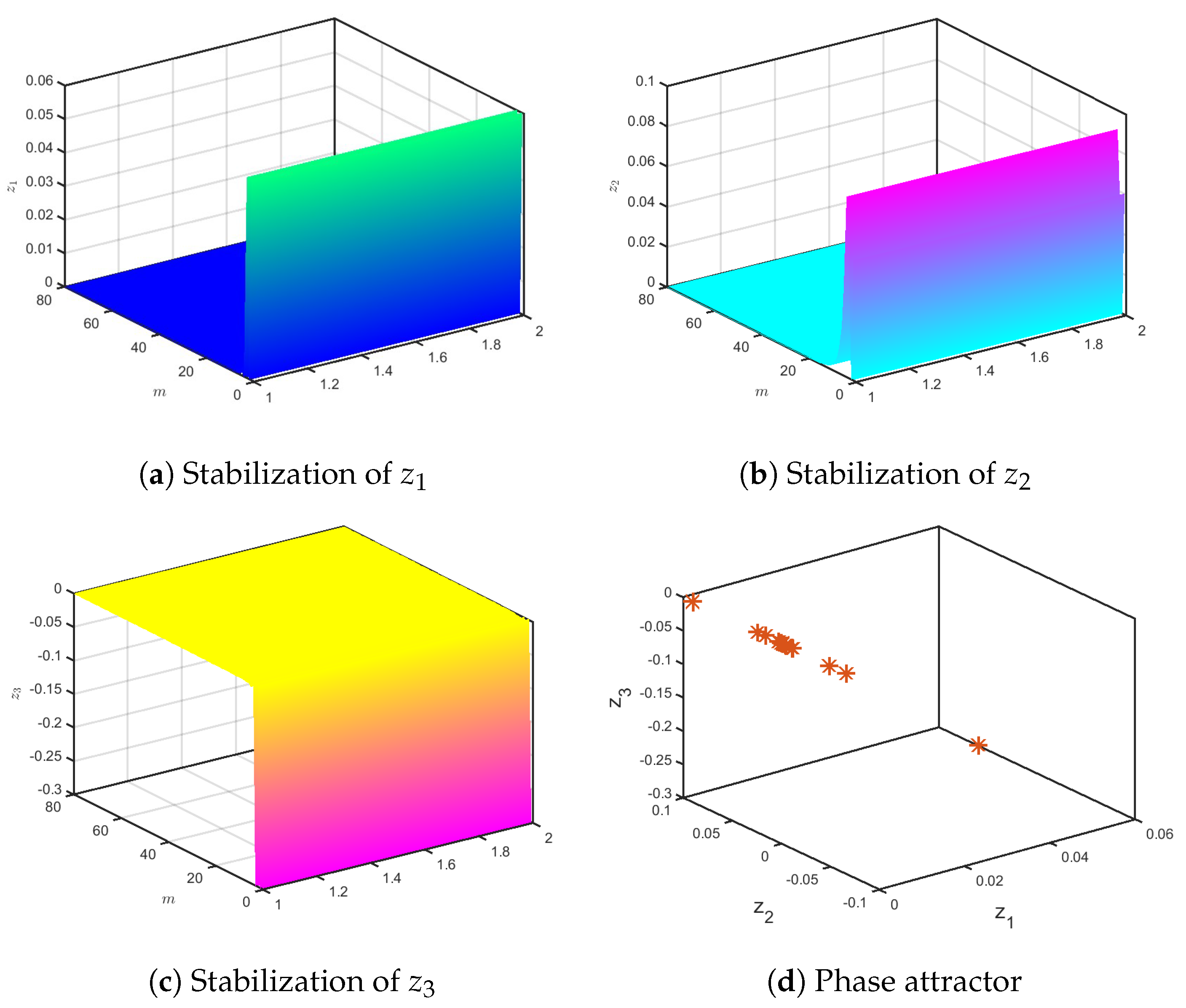
We can discuss the convergence of the commensurate chaotic multi-sigmoidal maps over time using numerical simulations performed on Proposition 1 to present the results. Specifically, Figure 14 and Figure 15 show the attractor and dynamic states of the controlled (21) for $\omega =0.92$ and $\omega =0.98$, respectively, with ${\rho }_1=0.1$, ${\rho }_2=1.78,$${\rho }_4=-1,$${\rho }_5=1$ and IC, ${\rho }_3=0.1,$$\sigma =0.5$, the fractional map approaches (0,0,0) asymptotically. Thus, the commensurate chaotic multi-sigmoidal map (1) is stabilized.

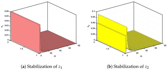
Figure 14. The evolution states of the controlled (21) for $\omega =0.92$.

Figure 15. The states of the controlled (21) for $\omega =0.98$.

5.2. The Incommensurate Chaos Control

In order to stabilize the proposed incommensurate multi-sigmoidal map (13), we use the following Lemma to provide the requirements for stability such that all states eventually attain zero:

Lemma 2

([30]). Consider the system

$$\left\{\begin{array}{c}{}^c\Delta _{\alpha }^{{\omega }_1}{z}_1\left(m\right)={\chi }_1\left(z(m-1+{\omega }_1)\right),\hfill \\ {}^c\Delta _{\alpha }^{{\omega }_2}{z}_2\left(m\right)={\chi }_2\left(z(m-1+{\omega }_2)\right),\hfill & \hfill {\omega }_i\in (0,1],\forall i=\overline{1,n}\hspace{1em}m=0,1,\cdots ,\\ ⋮\hfill \\ {}^c\Delta _{\alpha }^{{\omega }_n}{z}_n\left(m\right)={\chi }_n\left(z(m-1+{\omega }_n)\right).\hfill \end{array}\right.$$

(25)

where $\chi =({\chi }_1,\dots ,{\chi }_n):{\mathbb{R}}^n\to {\mathbb{R}}^n$, $z\left(m\right)={(z_1\left(m\right),\dots ,z_n\left(m\right))}^T\in {\mathbb{R}}^n$. Consider N as the (LCM) of the denominators ${\overline{\upsilon }}_i$ of ${\omega }_i$ with ${\omega }_i={\overline{\upsilon }}_i{\overline{u}}_i$, $({\overline{u}}_i,{\overline{\upsilon }}_i)=1$, ${\overline{\upsilon }}_i,{\overline{u}}_i\in {\mathbb{Z}}_{+}$,

$$det(diag({\lambda }^{\mathit{N}{\omega }_1},\cdots ,{\lambda }^{\mathit{N}{\omega }_n})-(1-{\lambda }^{\mathit{N}})\mathit{G})=0,$$

(26)

The Jacobian matrix of (25) is represented by G if $\mathbb{C}/K^{\mathit{s}}$ contains each root of (26).

$$K^{\mathit{s}}=\left\{\delta \in \mathbb{C}:\left|\delta \right|\le {\left(2cos{\displaystyle \frac{\left|arg\delta \right|}{s}}\right)}^s\mathit{and}\left|arg\delta \right|\le {\displaystyle \frac{s\pi }{2}}\right\},$$

(27)

with $\mathit{s}={\displaystyle \frac{1}{\mathit{N}}}$. Thus, the zero solution of (25) is asymptotically stable.

The 3D controlled map via incommensurate order is represented as

$$\left\{\begin{array}{cc}\hfill {}^c\Delta _{\alpha }^{{\omega }_1}{z}_1\left(m\right)& ={\displaystyle \frac{{\rho }_1}{1+e^{-\sigma z_1\left({\vartheta }_1\right)}}}+{\rho }_2{z}_1\left({\vartheta }_1\right)({\left(z_2\left({\vartheta }_1\right)\right)}^2-1)+\hfill \\ \hfill & {\displaystyle \frac{{\rho }_3}{1+e^{-\sigma z_3\left({\vartheta }_1\right)}}}-z_1\left({\vartheta }_1\right)+{\mathbf{C}}_1\left({\vartheta }_1\right),\hfill \\ \hfill {}^c\Delta _{\alpha }^{{\omega }_2}{z}_2\left(m\right)& =z_1\left({\vartheta }_2\right)+{\mathbf{C}}_2\left({\vartheta }_2\right),\hfill \\ \hfill {}^c\Delta _{\alpha }^{{\omega }_3}{z}_3\left(m\right)& ={\rho }_{4}sin\left(z_3\left({\vartheta }_3\right)\right)+{\displaystyle \frac{{\rho }_5}{1+e^{-\sigma z_1\left({\vartheta }_3\right)}}}-z_3\left({\vartheta }_3\right)+{\mathbf{C}}_3\left({\vartheta }_3\right).\hfill \end{array}\right.$$

(28)

Proposition 2.

The incommensurate multi-sigmoidal map (13) is controlled by the following 3D control law:

$$\left\{\begin{array}{ccc}\hfill {\mathit{C}}_1\left({\vartheta }_1\right)& ={\rho }_2{z}_1\left({\vartheta }_1\right)-{\displaystyle \frac{{\rho }_1}{1+e^{-\sigma z_1\left({\vartheta }_1\right)}}}-{\displaystyle \frac{{\rho }_3}{1+e^{-\sigma z_3\left({\vartheta }_1\right)}}}\hfill & \hfill -{\rho }_2{z}_1\left({\vartheta }_1\right){\left(z_2\left({\vartheta }_1\right)\right)}^2\\ \hfill {\mathit{C}}_2\left({\vartheta }_2\right)& =-{\displaystyle \frac{1}{2}}{z}_2\left({\vartheta }_2\right)\hfill \\ \hfill {\mathit{C}}_3\left({\vartheta }_3\right)& =-{\displaystyle \frac{{\rho }_5}{1+e^{-\sigma z_1\left({\vartheta }_3\right)}}}-{\rho }_{4}sin\left(z_3\left({\vartheta }_3\right)\right).\hfill \end{array}\right.$$

(29)

Proof. 

We discuss the robustness of the controller in the presence of incommensurate fractional-order variations in two cases. Firstly, substituting (29) into (28) yields the subsequent system

$$\left\{\begin{array}{cc}\hfill {}^c\Delta _{\alpha }^{{\omega }_1}{z}_1\left(m\right)& =-z_1\left({\vartheta }_1\right),\hfill \\ \hfill {}^c\Delta _{\alpha }^{{\omega }_3}{z}_2\left(m\right)& =z_1\left({\vartheta }_2\right)-{\displaystyle \frac{1}{2}}{z}_2\left({\vartheta }_2\right),\hfill \\ \hfill {}^c\Delta _{\alpha }^{{\omega }_3}{z}_3\left(m\right)& =-z_3\left({\vartheta }_3\right).\hfill \end{array}\right.$$

(30)

So,

$$det\left(diag({\lambda }^{\mathbf{N}{\omega }_1},{\lambda }^{\mathbf{N}{\omega }_2},{\lambda }^{\mathbf{N}{\omega }_3})\right)-(1-{\lambda }^{\mathbf{N}})G)=0,$$

where

$$\mathbf{G}=\left(\begin{array}{ccc}-1& 0& 0\\ 1& -{\displaystyle \frac{1}{2}}& 0\\ 0& 0& -1\end{array}\right),$$

(31)

Case 1: Let us consider $({\omega }_1,{\omega }_2,{\omega }_3)=(0.85,0.9,0.5)$, with $\mathbf{N}=20$,

$$det\left(\left(\begin{array}{ccc}{\lambda }^{17}& 0& 0.\\ 0& {\lambda }^{18}& 0\\ 0& 0& {\lambda }^{10}\end{array}\right)-\left(1-{\lambda }^{20}\right)\mathbf{G}\right)=0,$$

⇔

$$\begin{array}{cc}\hfill & 1.5{\lambda }^{40}-2{\lambda }^{38}-{\lambda }^{37}+{\lambda }^{35}-{\lambda }^{30}+{\lambda }^{28}+0.5{\lambda }^{27}-1.5{\lambda }^{20}+{\lambda }^{18}+0.5{\lambda }^{17}+0.5{\lambda }^{10}+0.5=0.\hfill \end{array}$$

(32)

Inevitably, ${\lambda }_j\in \mathbb{C}/K^{{\displaystyle \frac{1}{20}}},(j=1,\dots ,40)$ so that $\left|arg{\lambda }_j\right|>{\displaystyle \frac{\pi }{40}}$. Therefore, the map (28) satisfies the condition for being locally asymptotically stable based on Lemma 2.

Case 2: For $({\omega }_1,{\omega }_2,{\omega }_3)=(1,0.85,0.5)$ and $\mathbf{N}=100$,

$$det\left(\left(\begin{array}{ccc}{\lambda }^{100}& 0& 0.\\ 0& {\lambda }^{85}& 0\\ 0& 0& {\lambda }^{50}\end{array}\right)-\left(1-{\lambda }^{100}\right)\mathbf{G}\right)=0,$$

⇔

$$\begin{array}{cc}\hfill & 0.5{\lambda }^{200}-{\lambda }^{185}-0.5{\lambda }^{150}+{\lambda }^{135}-{\lambda }^{100}+{\lambda }^{85}+0.5{\lambda }^{50}+0.5=0.\hfill \end{array}$$

(33)

According to Lemma 2, the map (28) asymptotically stabilizes toward zero equilibrium since ${\lambda }_j\in \mathbb{C}/K^{{\displaystyle \frac{1}{100}}},(j=1,\dots ,200)$.□

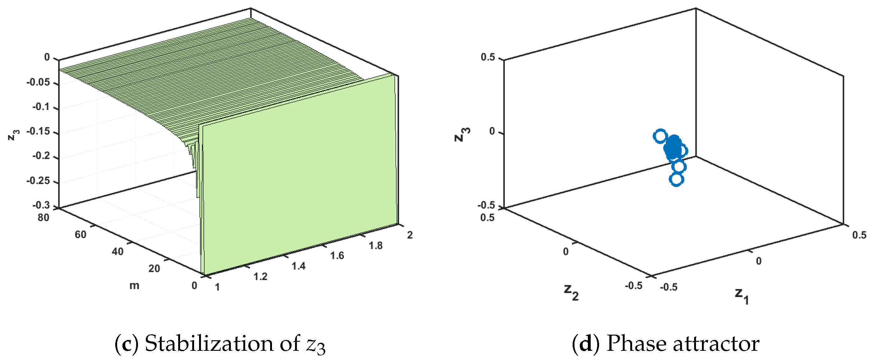
As seen in Figure 16 and Figure 17, the controlled map (28) for $({\omega }_1,{\omega }_2,{\omega }_3)=(0.85,0.9,0.5)$ and $({\omega }_1,{\omega }_2,{\omega }_3)=(1,0.85,0.5)$ has stabilized. Hence, we can see that the novel incommensurate chaotic multi-sigmoidal map is stabilized.

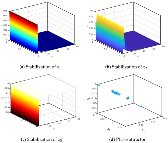
Figure 16. The evolution states of the controlled (28) for $({\omega }_1,{\omega }_2,{\omega }_3)=(0.85,0.9,0.5)$.

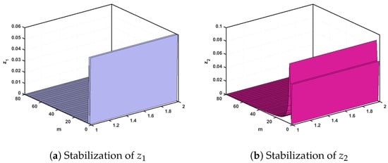
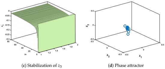
Figure 17. The evolution states of the controlled (28) for $({\omega }_1,{\omega }_2,{\omega }_3)=(1,0.85,0.5)$.

6. Conclusions

In this paper, a novel fractional multi-sigmoidal map was introduced. The behavior of the map is affected by its fractional derivative and factors system, which we carefully examined in commensurate orders and incommensurate orders.

Firstly, the numerical study of the map without an equilibrium point further emphasizes the system’s capacity to exhibit a wide variety of hidden dynamical motion, which reveals asymmetry when the parameters or derivative fractional values are varied. Moreover, the $C_0$ complexity and the approximation entropy $ApEn$ are employed to quantitatively assess the chaotic complexity of fractional multi-sigmoidal maps. In addition, we establish effective control mechanisms that maintain map stabilization and advance them in the direction of asymptotic zero. The most important results of this investigation confirm that the commensurate multiple sigmoidal map’s chaotic behavior is less complex than that of the incommensurate multiple sigmoidal map because of the considerable adaptability of the fractional derivatives. As a result, the incommensurate derivative improves chaotic predictions and greatly increases the complexity of the map state space.

Future research can take into account maps based on multi-sigmoidal functions, such as the triple and quadruple sigmoidal functions of the system, in order to better understand the effects of fractional chaotic multiple sigmoidal systems, to further the study of chaotic dynamical systems, like physics and encryption, and to examine their effects on the system dynamics and control performance in greater detail.

References

- Hamadneh, T.; Hioual, A.; Alsayyed, O.; Al-Khassawneh, Y.A.; Al-Husban, A.; Ouannas, A. The FitzHugh–Nagumo Model Described by Fractional Difference Equations: Stability and Numerical Simulation. Axioms 2023, 12, 806. [Google Scholar] [CrossRef]
- Ferreira, R.A. Discrete Fractional Calculus and Fractional Difference Equations; Springer: Cham, Switzerland, 2022. [Google Scholar]
- Kumar, S.; Matouk, A.E.; Chaudhary, H.; Kant, S. Control and synchronization of fractional-order chaotic satellite systems using feedback and adaptive control techniques. Int. J. Adapt. Control Signal Process. 2021, 35, 484–497. [Google Scholar] [CrossRef]
- Li, H.L.; Cao, J.; Hu, C.; Jiang, H.; Alsaadi, F.E. Synchronization analysis of discrete-time fractional-order quaternion-valued uncertain neural networks. IEEE Trans. Neural Netw. Learn. Syst. 2023, 35, 14178–14189. [Google Scholar] [CrossRef] [PubMed]
- Avazzadeh, Z.; Nikan, O.; Nguyen, A.T. A localized hybrid kernel meshless technique for solving the fractional Rayleigh–Stokes problem for an edge in a viscoelastic fluid. Eng. Anal. Bound. Elem. 2023, 146, 695–705. [Google Scholar] [CrossRef]
- Ouannas, A.; Khennaoui, A.A.; Momani, S.; Pham, V.T.; El-Khazali, R. Hidden attractors in a new fractional–order discrete system: Chaos, complexity, entropy, and control. Chin. Phys. B 2020, 29, 050504. [Google Scholar] [CrossRef]
- Ahmadi, A.; Parthasarathy, S.; Pal, N.; Rajagopal, K.; Jafari, S.; Tlelo-Cuautle, E. Extreme multistability and extreme events in a novel chaotic circuit with hidden attractors. Int. J. Bifurc. Chaos 2022, 33, 2330016. [Google Scholar] [CrossRef]
- Peng, Y.; Lan, Z.; Li, W.; Li, Y.; Peng, J. Modeling different discrete memristive sine maps and its parameter identification. Eur. Phys. J. Spec. Top. 2022, 231, 3187–3196. [Google Scholar] [CrossRef]
- Diabi, L.; Ouannas, A.; Hioual, A.; Grassi, G.; Momani, S. The Discrete Ueda System and Its Fractional Order Version: Chaos, Stabilization and Synchronization. Mathematics 2025, 13, 239. [Google Scholar] [CrossRef]
- Baione, F.; Biancalana, D.; De Angelis, P. An application of Sigmoid and Double-Sigmoid functions for dynamic policyholder behaviour. Decis. Econ. Financ. 2021, 44, 5–22. [Google Scholar] [CrossRef]
- Mulimani, M.; Kumbinarasaiah, S. Gegenbauer wavelets collocation technique for the nonlinear Fisher’s reaction–diffusion equation with application arising in biological and chemical sciences. Int. J. Dyn. Control 2025, 13, 15. [Google Scholar] [CrossRef]
- Mfungo, D.E.; Fu, X.; Wang, X.; Xian, Y. Enhancing image encryption with the Kronecker Xor product, the Hill Cipher, and the Sigmoid Logistic Map. Appl. Sci. 2023, 13, 4034. [Google Scholar] [CrossRef]
- Pratiwi, H.; Windarto, A.P.; Susliansyah, S.; Aria, R.R.; Susilowati, S.; Rahayu, L.K.; Fitriani, Y.; Merdekawati, A.; Rahadjeng, I.R. Sigmoid activation function in selecting the best model of artificial neural networks. J. Phys. Conf. Ser. 2020, 1471, 012010. [Google Scholar] [CrossRef]
- Martinelli, C.; Coraddu, A.; Cammarano, A. Approximating piecewise nonlinearities in dynamic systems with sigmoid functions: Advantages and limitations. Nonlinear Dyn. 2023, 111, 8545–8569. [Google Scholar] [CrossRef]
- Jiang, H.G.; Jia, M.M. Chaos control for multi-scroll chaotic attractors generated by introducing a bipolar sigmoid function series. Indian J. Phys. 2020, 94, 851–861. [Google Scholar] [CrossRef]
- Al-Taani, H.; Abu Hammad, M.M.; Abudayah, M.; Diabi, L.; Ouannas, A. On Fractional Discrete Memristive Model with Incommensurate Orders: Symmetry, Asymmetry, Hidden Chaos and Control Approaches. Symmetry 2025, 17, 143. [Google Scholar] [CrossRef]
- Khennaoui, A.A.; Ouannas, A.; Boulaaras, S.; Pham, V.T.; Taher Azar, A. A fractional map with hidden attractors: Chaos and control. Eur. Phys. J. Spec. Top. 2020, 229, 1083–1093. [Google Scholar] [CrossRef]
- Elaskar, S. Symmetry in Nonlinear Dynamics and Chaos. Symmetry 2022, 15, 102. [Google Scholar] [CrossRef]
- Wang, R.; Li, C.; Kong, S.; Jiang, Y.; Lei, T. A 3D memristive chaotic system with conditional symmetry. Chaos Solitons Fractals 2022, 158, 111992. [Google Scholar] [CrossRef]
- Leutcho, G.D.; Wang, H.; Kengne, R.; Kengne, L.K.; Njitacke, Z.T.; Fozin, T.F. Symmetry-breaking, amplitude control and constant Lyapunov exponent based on single parameter snap flows. Eur. Phys. J. Spec. Top. 2022, 230, 1887–1903. [Google Scholar] [CrossRef]
- Thoai, V.P.; Pham, V.T.; Grassi, G.; Momani, S. Assessing sigmoidal function on memristive maps. Heliyon 2024, 10, e27781. [Google Scholar] [CrossRef] [PubMed]
- Anastassiou, G.A. General multiple sigmoid functions relied complex valued multivariate trigonometric and hyperbolic neural network approximations. RGMIA Res. Rep. Coll. 2023, 26, 43. [Google Scholar]
- Abdeljawad, T. On Riemann and Caputo fractional differences. Comput. Math. Appl. 2011, 62, 1602–1611. [Google Scholar] [CrossRef]
- Atici, F.M.; Eloe, P. Discrete fractional calculus with the nabla operator. Electron. J. Qual. Theory Differ. Equ. 2009, 62. [Google Scholar] [CrossRef]
- Wu, G.C.; Baleanu, D. Discrete fractional logistic map and its chaos. Nonlinear Dyn. 2014, 75, 283–287. [Google Scholar] [CrossRef]
- Wu, G.C.; Baleanu, D. Jacobian matrix algorithm for Lyapunov exponents of the discrete fractional maps. Commun. Nonlinear Sci. Numer. Simul. 2015, 22, 95–100. [Google Scholar] [CrossRef]
- Richman, J.S.; Moorman, J.R. Physiological time-series analysis using approximate entropy and sample entropy. Am. J. Physiol.-Heart Circ. Physiol. 2000, 278, H2039–H2049. [Google Scholar] [CrossRef] [PubMed]
- Shen, E.-H.; Cai, Z.-J.; Gu, F.-J. Mathematical foundation of a new complexity measure. Appl. Math. Mech. 2005, 26, 1188–1196. [Google Scholar]
- Cermák, J.; Győri, I.; Nechvátal, L. On explicit stability conditions for a linear fractional difference system. Fract. Calc. Appl. Anal. 2015, 18, 651–672. [Google Scholar] [CrossRef]
- Shatnawi, M.T.; Djenina, N.; Ouannas, A.; Batiha, I.M.; Grassi, G. Novel convenient conditions for the stability of nonlinear incommensurate fractional-order difference systems. Alex. Eng. J. 2022, 61, 1655–1663. [Google Scholar] [CrossRef]
Disclaimer/Publisher’s Note: The statements, opinions and data contained in all publications are solely those of the individual author(s) and contributor(s) and not of MDPI and/or the editor(s). MDPI and/or the editor(s) disclaim responsibility for any injury to people or property resulting from any ideas, methods, instructions or products referred to in the content. |
© 2025 by the authors. Licensee MDPI, Basel, Switzerland. This article is an open access article distributed under the terms and conditions of the Creative Commons Attribution (CC BY) license (https://creativecommons.org/licenses/by/4.0/).