The Sine Alpha Power-G Family of Distributions: Characterizations, Regression Modeling, and Applications

Abstract

This study develops a new method for generating families of distributions based on the alpha power transformation and the trigonometric function, which enables enormous versatility in the resulting sub-models and enhances the ability to more accurately characterize tail shapes. This proposed family of distributions is characterized by a single parameter, which exhibits considerable flexibility in capturing asymmetric datasets, making it a valuable alternative to some families of distributions that require additional parameters to achieve similar levels of flexibility. The sine alpha power generated family is introduced using the proposed method, and some of its members and properties are discussed. A particular member, the sine alpha power-Weibull (SAP-W), is investigated in depth. Graphical representations of the new distribution display monotone and non-monotone forms, whereas the hazard rate function takes a reversed J shape, J shape, bathtub, increasing, and decreasing shapes. Various characteristics of SAP-W distribution are derived, including moments, rényi entropies, and order statistics. Parameters of SAP-W are estimated using the maximum likelihood technique, and the effectiveness of these estimators is examined via Monte Carlo simulations. The superiority and potentiality of the proposed approach are demonstrated by analyzing three real-life engineering applications. The SAP-W outperforms several competing models, showing its flexibility. Additionally, a novel-log location-scale regression model is presented using SAP-W. The regression model’s significance is illustrated through its application to real data.

1. Introduction

Stochastic distributions are widely employed to forecast and explain situations that occur in the real world. Several statistical distributions have been predicted and utilized to fit real-world data in several fields, such as economics, environmental sciences, actuarial sciences, engineering, finance, architecture, biological research, and medical sciences. However, in several of these disciplines, the data might indicate a complex trend that classical and conventional distributions cannot adequately explain. Therefore, numerous researchers have tried to expand the classical distribution and create various new families of distributions to increase the flexibility and adaptability to fit data from multiple fields of study. The literature has investigated several techniques for creating new families of distributions. These include the exponentiated family by [1], the T-X generalized family by [2], which proposes a novel technique for generating families of distributions, and the alpha power transformation (APT) family of distributions [3]. The cumulative distribution function (CDF) and the probability density function (PDF) of APT the family can be expressed as

$$F_{APT}\left(x\right)=\left\{\begin{array}{ccc}\hfill {\displaystyle \frac{{\alpha }^{F\left(x\right)}-1}{\alpha -1}}& \mathrm{if}\hfill & \alpha >0,\alpha \ne 1,\hfill \\ \hfill F\left(x\right)& \mathrm{if}\hfill & \alpha =1,\hfill \end{array}\right.$$

(1)

$$f_{APT}\left(x\right)=\left\{\begin{array}{ccc}\hfill {\displaystyle \frac{log\alpha }{\alpha -1}}f\left(x\right){\alpha }^{F\left(x\right)}& \mathrm{if}\hfill & \alpha >0,\alpha \ne 1,\hfill \\ \hfill f\left(x\right)& \mathrm{if}\hfill & \alpha =1,\hfill \end{array}\right.$$

(2)

where $F\left(x\right)$ and $f\left(x\right)$ are the CDF and PDF of only continuous distribution.

This technique has been applied in several studies to introduce new distributions, including the APT approach used for the exponential distribution in [3], the alpha power Weibull distribution presented in [4], the alpha power Pareto distribution introduced in [5], the alpha power Fréchet distribution provided in [6], and the alpha power inverted Topp–leone distribution supplied in [7].

In recent years, extensive research has been conducted to identify the perfect distribution for representing data, and the trigonometric transformation has been suggested as an appropriate choice. The trigonometric function provides adaptability and flexibility as the parameter(s) oscillate as their value changes, and the periodic function controls the way the distribution curve behaves. Combining several functions with varying behaviors provides a better framework for modeling real data, which was lacking in some generalized statistical distributions [8,9]. The appropriate mixing of trigonometric transformation and generalized distributions will produce an ideal model with better goodness of fit (GoF) for data in many real-world situations. Recently, the studies of [10,11] proposed a new technique to create a novel family of distributions called the sine-G (SG) family. Suppose that $F\left(x\right)$ and $f\left(x\right)$ are the CDF and PDF of any continuous distribution. Then, the CDF and PDF of the SG are given, respectively, as follows:

$$G\left(x\right)=sin\left[{\displaystyle \frac{\pi }{2}}F\left(x\right)\right],x\in \mathbb{R},$$

(3)

$$g\left(x\right)={\displaystyle \frac{\pi }{2}}f\left(x\right)cos\left[{\displaystyle \frac{\pi }{2}}F\left(x\right)\right],x\in \mathbb{R}.$$

(4)

Several studies have used the trigonometric transformation to introduce new families of distribution. Examples include the cos-G proposed in [11,12], the tan-G in [11,13], the sec-G in [11,14], the sine Topp–Leone-G in [15], the sine Kumaraswamy-G in [16], the arctan-X in [17], the sine exponentiated Weibull-H in [18], the sine truncated Lomax distribution in [19], the extended cosine generalized family of distributions in [20], the cosine Topp–Leone family of distributions in [9], the exponentiated cos-G and exponentiated tan-G in [21], the secant Kumaraswamy family of distributions in [22], the tan Weibull loss distribution in [23], the novel sin-G in [24], the exponentiated arctan-X family of distributions in [25], the new sine family of distributions in [26], and the sine type II Topp–Leone-G family of distributions in [8], among others.

In this paper, we discuss a distinct family known as the sine alpha power generated (SAP-G) family, which is based on combining the sine-G and alpha power transformations. We are introducing this new family primarily with the following objectives:

• Create new models with significant graphical and mathematical features.
• Expand the classical distributions by adding only one parameter instead of two or more.
• Create family submodels that possess only one additional parameter, circumventing issues related to over-parameterization.
• Include the trigonometric function, which increases the flexibility of the submodels, resulting in new and more adaptable models.
• Contribute to the existing literature on trigonometric families by presenting a novel family of distributions that can enhance the adaptability of already existing distributions with the ideal number of parameters.

Furthermore, five members of the SAP-G family are presented, with an emphasis on the SAP-W distribution and its properties. The SAP-W distribution demonstrates different curve shapes for its density and hazard rate function, showing its flexibility and usefulness for modeling real-world data in several application disciplines. In addition, the SAP-W distribution provides a superior fit compared to five competing models using three real-world engineering applications. Additionally, a new log-location-scale regression model is introduced.

The remainder of the paper is organized as follows. Section 2 discusses the SAP-G family and some of its features. Section 3 introduces the SAP-W distribution and investigates some fundamental statistical properties. The parameters of SAP-W are estimated using the maximum likelihood method in Section 4. In Section 5, we provide a simulation study to examine the performance of the estimates. In Section 6, three real-life engineering data sets are analyzed to illustrate the superiority of the SAP-W distribution. A regression model for SAP-W is proposed, and its efficiency is determined using real-world data in Section 7. Finally, the conclusion is presented in Section 8.

2. The Sine Alpha Power Generated Family

Let X be a random variable (RV) from SAP-G with CDF G(X). Therefore, G(X) of the SAP-G family can easily be derived by substituting F(x) in (3) with (1) as follows:

$$G\left(x\right)=sin\left[{\displaystyle \frac{\pi }{2}}\left({\displaystyle \frac{1-{\alpha }^{F\left(x\right)}}{1-\alpha }}\right)\right],x\in \mathbb{R},\alpha >0,\alpha \ne 1,$$

(5)

with the PDF $g\left(x\right)$ given by

$$g\left(x\right)={\displaystyle \frac{\pi }{2}}{\displaystyle \frac{log\alpha }{(\alpha -1)}}{\alpha }^{F\left(x\right)}f\left(x\right)cos\left[{\displaystyle \frac{\pi }{2}}\left({\displaystyle \frac{1-{\alpha }^{F\left(x\right)}}{1-\alpha }}\right)\right],$$

(6)

where $F\left(x\right)$ and $f\left(x\right)$ represent the CDF and PDF for various distributions, respectively. We can derive the hazard rate function, h(x), of the SAP-G by

$$h\left(x\right)={\displaystyle \frac{\pi }{2}}{\displaystyle \frac{log\alpha }{(\alpha -1)}}{\alpha }^{F\left(x\right)}f\left(x\right){\displaystyle \frac{cos\left[\frac{\pi }{2}\left(\frac{1-{\alpha }^{F\left(x\right)}}{1-\alpha }\right)\right]}{1-sin\left[\frac{\pi }{2}\left(\frac{1-{\alpha }^{F\left(x\right)}}{1-\alpha }\right)\right]}}.$$

(7)

The survival function of the SAP-G, s(x), can be written as

$$s\left(x\right)=1-sin\left[{\displaystyle \frac{\pi }{2}}\left({\displaystyle \frac{1-{\alpha }^{F\left(x\right)}}{1-\alpha }}\right)\right].$$

(8)

Inverting (5) produces the SAP-G family’s quantile function, as displayed below:

$$Q\left(u\right)=F^{-1}\left[{\displaystyle \frac{log\left(1-\frac{2(1-\alpha )arcsin\left(u\right)}{\pi }\right)}{log\alpha }}\right],$$

(9)

where $u\in (0,1)$. Random numbers from SAP-G can be generated using (9).

2.1. Members of the SAP-G Family

The SAP-G may add more flexibility to various standard distributions and improve their efficiency and adaptability in their applications. This section produced several types of distributions. The following sections describe some of the members.

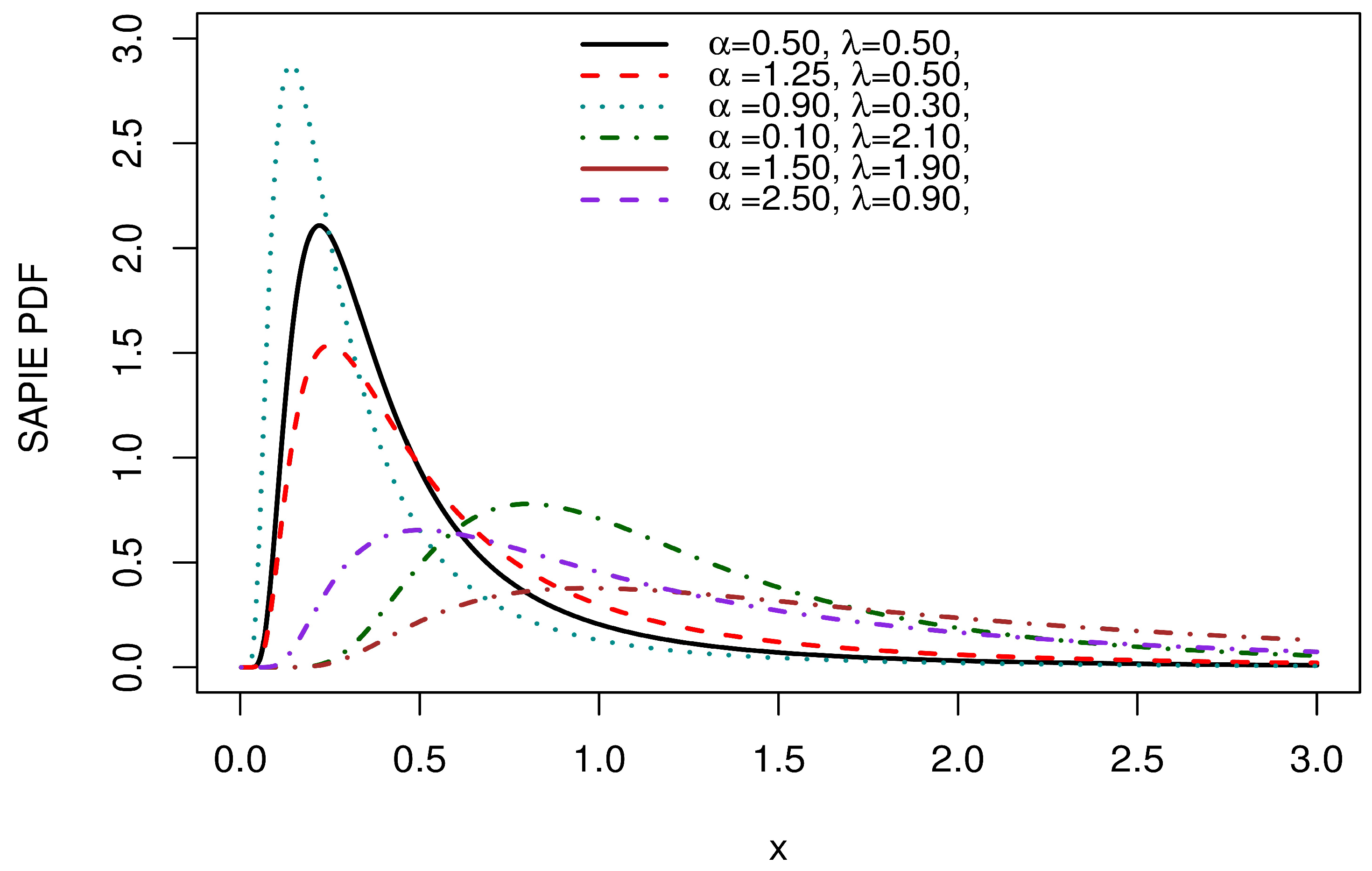
2.1.1. Sine Alpha Power Weibull Distribution

As indicated by its name, the SAP-W is a member of the SAP-G family of distributions. To describe this new member, we define $F\left(x\right)$ in (5) as the CDF of the Weibull distribution; then, the CDF of SAP-W is

$$G\left(x\right)=sin\left[{\displaystyle \frac{\pi }{2}}\left({\displaystyle \frac{1-{\alpha }^{1-e^{-\lambda x^{\beta }}}}{1-\alpha }}\right)\right],x,\alpha ,\lambda ,\beta >0,\alpha \ne 1.$$

(10)

The corresponding PDF is expressed as follows:

$$g\left(x\right)={\displaystyle \frac{\pi }{2}}{\displaystyle \frac{\lambda \beta (log\alpha )}{(\alpha -1)}}{x}^{\beta -1}{e}^{-\lambda x^{\beta }}{\alpha }^{1-e^{-\lambda x^{\beta }}}cos\left[{\displaystyle \frac{\pi }{2}}\left({\displaystyle \frac{1-{\alpha }^{1-e^{-\lambda x^{\beta }}}}{1-\alpha }}\right)\right].$$

(11)

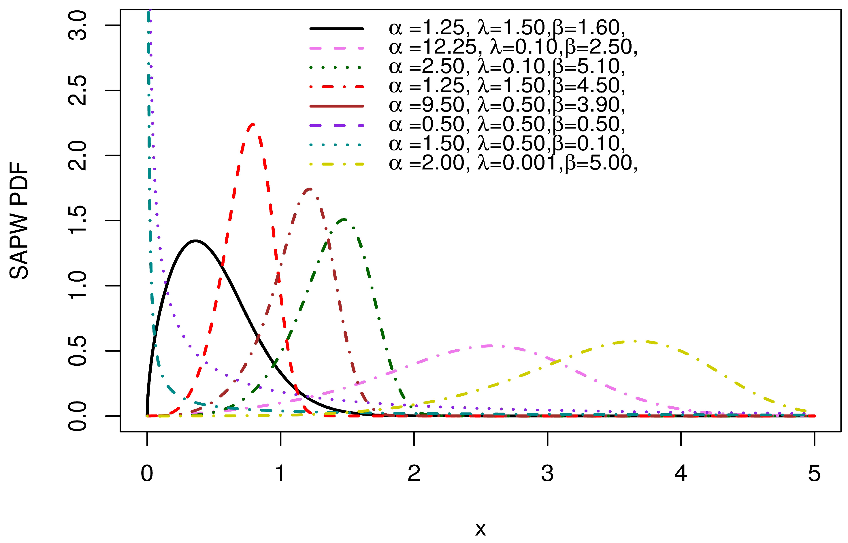
Plots of various PDF forms for the SAP-W family are presented in Figure 1. It is apparent that the PDF takes on approximately symmetrical patterns, skewed to the right and left, and decreasing shapes.

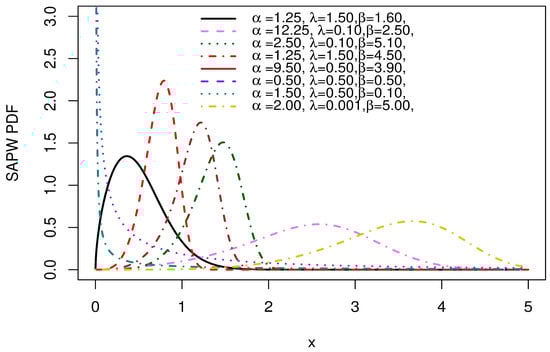
Figure 1. PDF plots of the SAP-W.

2.1.2. Sine Alpha Power Exponential Distribution

Using the exponential distribution, the CDF of the sine alpha power exponential (SAP-E) is given as follows:

$$G\left(x\right)=sin\left[{\displaystyle \frac{\pi }{2}}\left({\displaystyle \frac{1-{\alpha }^{1-e^{-\lambda x}}}{1-\alpha }}\right)\right],x,\alpha ,\lambda >0,\alpha \ne 1,$$

and the SAP-E PDF is

$$g\left(x\right)={\displaystyle \frac{\pi }{2}}{\displaystyle \frac{\lambda log\alpha }{(\alpha -1)}}{e}^{-\lambda x}{\alpha }^{1-e^{-\lambda x}}cos\left[{\displaystyle \frac{\pi }{2}}\left({\displaystyle \frac{1-{\alpha }^{1-e^{-\lambda x}}}{1-\alpha }}\right)\right].$$

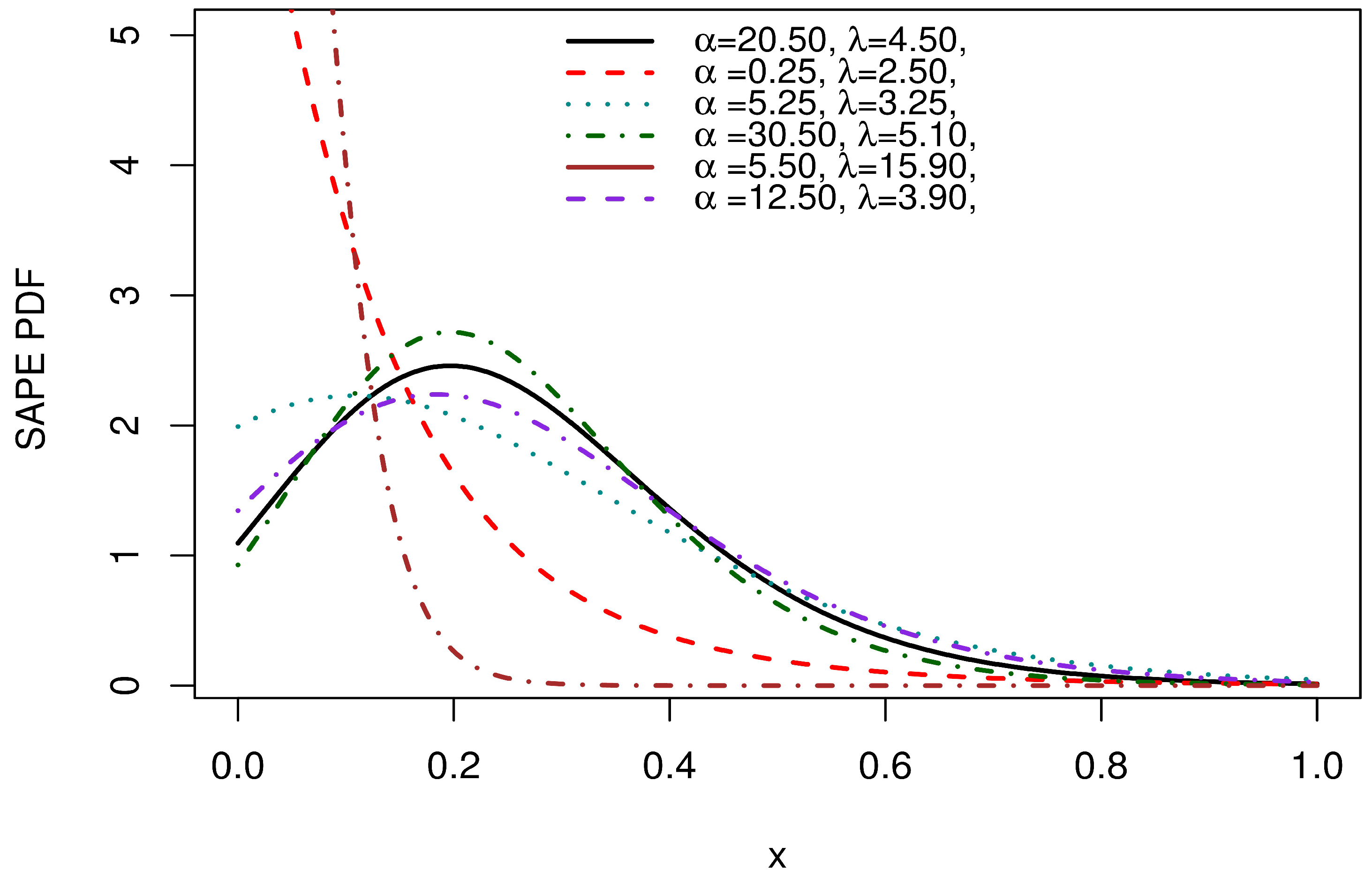
Figure 2 displays several PDF forms for SAP-E. The PDF of the SAP-E is decreasing and right-skewed.

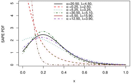
Figure 2. PDF plots of the SAP-E.

2.1.3. Sine Alpha Power Inverse Exponential Distribution

The inverse exponential distribution can be used to obtain the CDF and PDF of the sine alpha power inverse exponential (SAP-IE) as follows:

$$G\left(x\right)=sin\left[{\displaystyle \frac{\pi }{2}}\left({\displaystyle \frac{1-{\alpha }^{e^{-(\frac{\lambda }{x})}}}{1-\alpha }}\right)\right],x,\alpha ,\lambda >0,\alpha \ne 1,$$

$$g\left(x\right)={\displaystyle \frac{\pi }{2}}{\displaystyle \frac{\lambda log\alpha }{(\alpha -1)}}{x}^{-2}{e}^{-({\displaystyle \frac{\lambda }{x}})}{\alpha }^{e^{-({\displaystyle \frac{\lambda }{x}})}}cos\left[{\displaystyle \frac{\pi }{2}}\left({\displaystyle \frac{1-{\alpha }^{e^{-(\frac{\lambda }{x})}}}{1-\alpha }}\right)\right].$$

Figure 3 exhibits right-skewed forms of the SAP-IE density.

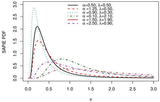
Figure 3. Density plots of the SAP-IE.

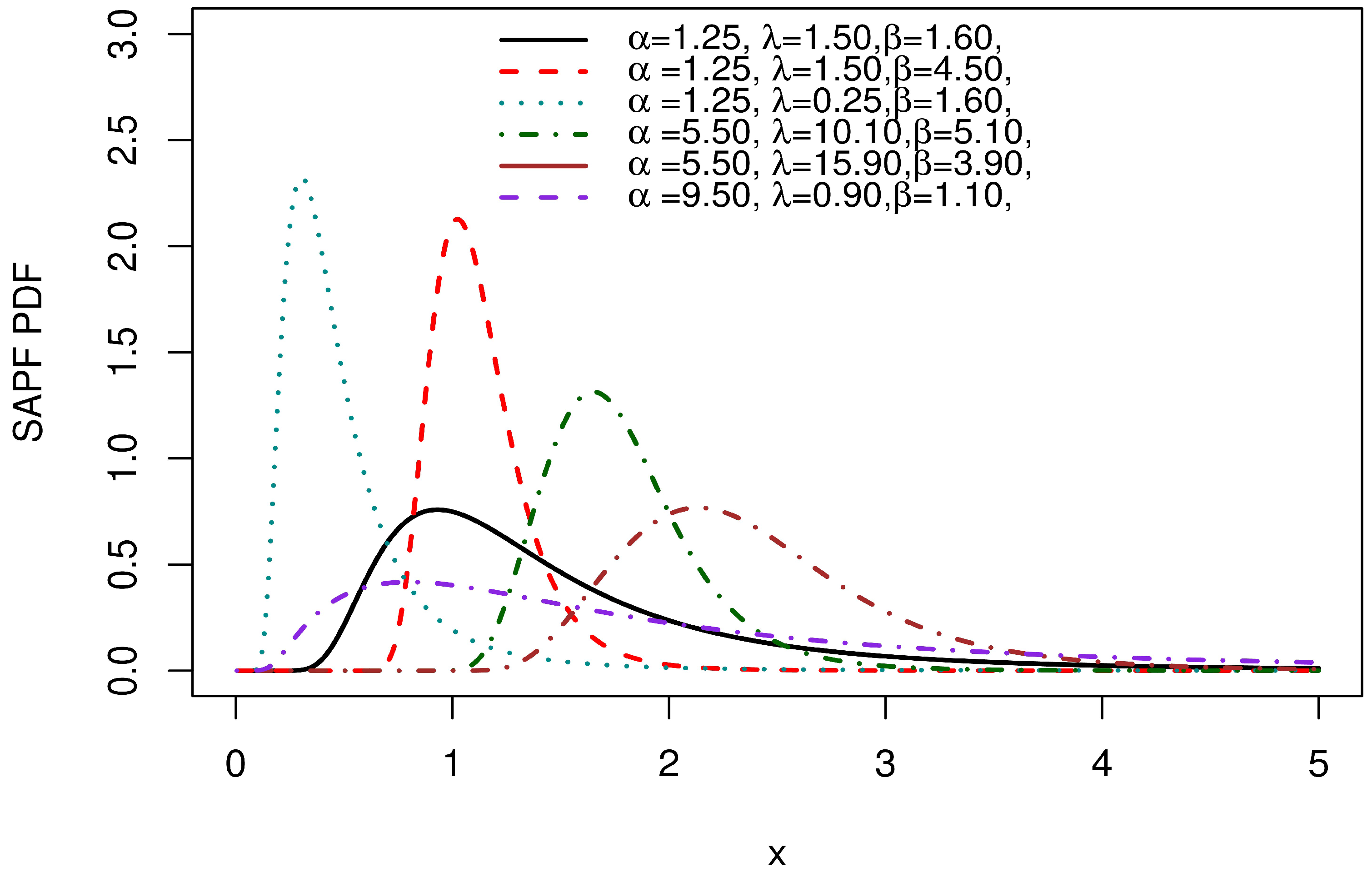
2.1.4. Sine Alpha Power Fréchet Distribution

The CDF and PDF of the sine alpha power fréchet (SAP-F) are obtained as follows:

$$G\left(x\right)=sin\left[{\displaystyle \frac{\pi }{2}}\left({\displaystyle \frac{1-{\alpha }^{e^{-\lambda x^{-\beta }}}}{1-\alpha }}\right)\right],x,\alpha ,\lambda ,\beta >0,\alpha \ne 1,$$

$$g\left(x\right)={\displaystyle \frac{\pi }{2}}{\displaystyle \frac{\lambda \beta log\alpha }{(\alpha -1)}}{x}^{-(\beta +1)}{e}^{-\lambda x^{-\beta }}{\alpha }^{e^{-\lambda x^{-\beta }}}cos\left[{\displaystyle \frac{\pi }{2}}\left({\displaystyle \frac{1-{\alpha }^{e^{-\lambda x^{-\beta }}}}{1-\alpha }}\right)\right].$$

Figure 4 presents graphs of several PDF forms for SAP-F. The PDF can be displayed in both right-skewed and nearly symmetric forms.

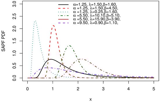
Figure 4. PDF plots of the SAP-F.

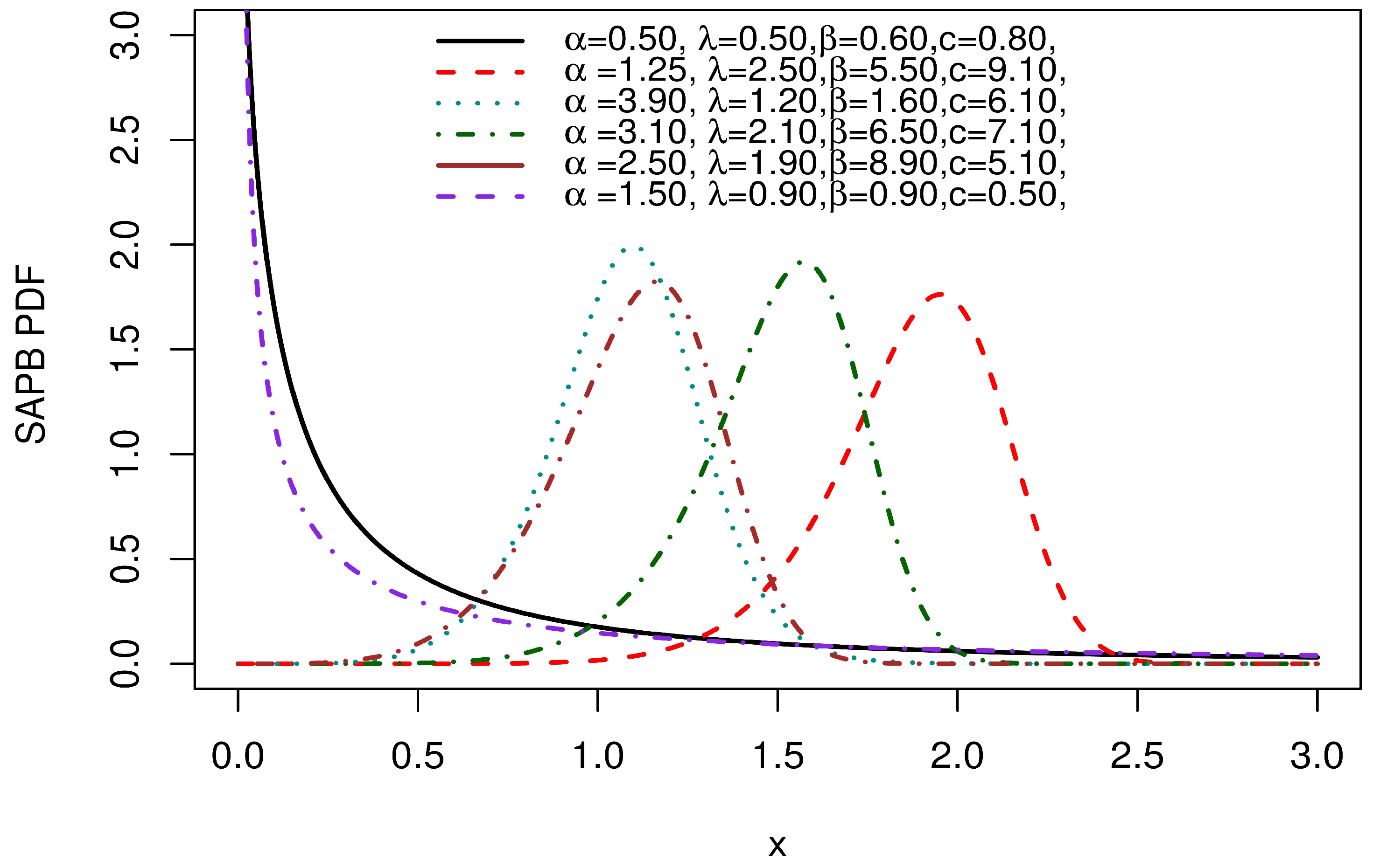
2.1.5. Sine Alpha Power Burr XII Distribution

The sine alpha power Burr XII (SAP-Burr XII) distribution is produced by applying the Burr XII distribution. Therefore, the CDF of SAP-B is

$$G\left(x\right)=sin\left[{\displaystyle \frac{\pi }{2}}\left({\displaystyle \frac{1-{\alpha }^{1-{[1+{(\frac{x}{\lambda })}^c]}^{-\beta }}}{1-\alpha }}\right)\right],x,\alpha ,\lambda ,c,\beta >0,\alpha \ne 1,$$

and the SAP-B PDF is

$$g\left(x\right)={\displaystyle \frac{\pi }{2}}{\displaystyle \frac{c\beta log\alpha }{\lambda (\alpha -1)}}{({\displaystyle \frac{x}{\lambda }})}^{c-1}{[1+{({\displaystyle \frac{x}{\lambda }})}^c]}^{-(\beta +1)}{\alpha }^{1-{[1+{({\displaystyle \frac{x}{\lambda }})}^c]}^{-\beta }}cos\left[{\displaystyle \frac{\pi }{2}}\left({\displaystyle \frac{1-{\alpha }^{1-{[1+{(\frac{x}{\lambda })}^c]}^{-\beta }}}{1-\alpha }}\right)\right],$$

Figure 5 indicates the PDF plots of the SAP-Burr XII. The PDF plots display approximately symmetrical forms, skewed to the right and left, and decreasing in form.

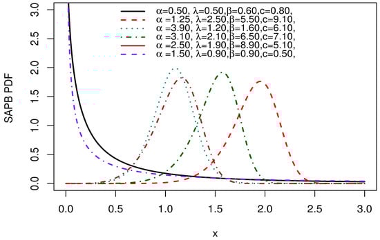
Figure 5. PDF plots of the SAP-Burr XII.

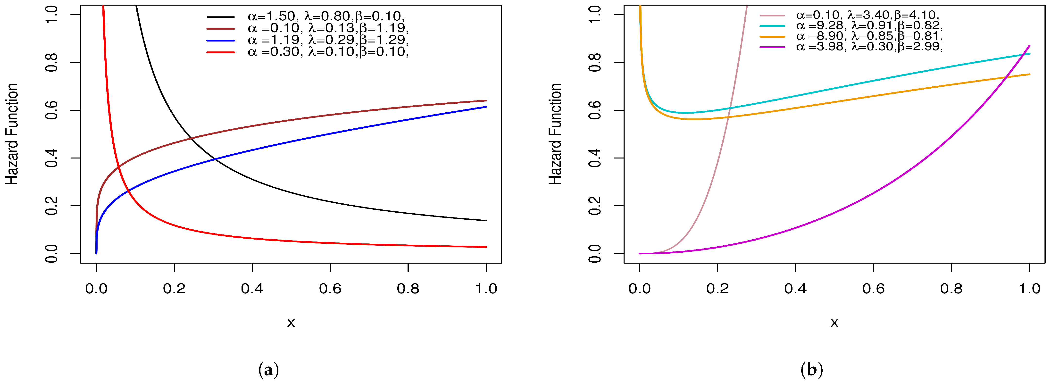
3. The Sine Alpha Power-Weibull Distribution

This section will investigate several statistical properties of the SAP-W distribution. The hazard, $h\left(x\right)$, and survival functions, $s\left(x\right)$, are, respectively, as follows:

$$h\left(x\right)={\displaystyle \frac{\pi }{2}}{\displaystyle \frac{\lambda \beta \left(log\alpha \right)}{(\alpha -1)}}{x}^{\beta -1}{e}^{-\lambda x^{\beta }}{\alpha }^{1-e^{-\lambda x^{\beta }}}{\displaystyle \frac{cos\left[\frac{\pi }{2}\left(\frac{1-{\alpha }^{1-e^{-\lambda x^{\beta }}}}{1-\alpha }\right)\right]}{1-sin\left[\frac{\pi }{2}\left(\frac{1-{\alpha }^{1-e^{-\lambda x^{\beta }}}}{1-\alpha }\right)\right]}},x,\alpha ,\lambda ,\beta >0,\alpha \ne 1.$$

(12)

$$s\left(x\right)=1-sin\left[{\displaystyle \frac{\pi }{2}}\left({\displaystyle \frac{1-{\alpha }^{1-e^{-\lambda x^{\beta }}}}{1-\alpha }}\right)\right],x,\alpha ,\lambda ,\beta >0,\alpha \ne 1.$$

(13)

The SAP-W hazard function in Figure 6 has a variety of forms, including increasing, decreasing, bathtub, reversed J-shaped, and J-shaped.

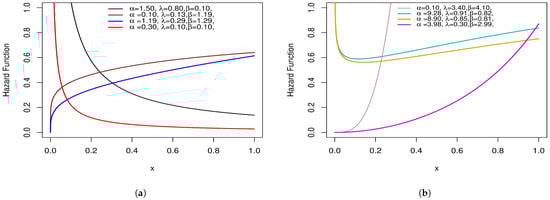
Figure 6. Hazard function plots of the SAP-W: (a) represents decreasing and reversed J-shaped; (b) represents increasing, bathtub, and J-shaped.

3.1. Expansion for the SAP-W Density

Using (11), the PDF of the SAP-W can be obtained as follows:

$$g\left(x\right)=\lambda \beta \sum _{j=0}^{\infty }{\psi }_j{x}^{\beta -1}{e}^{-(j+1)\lambda x^{\beta }},x,\alpha ,\lambda ,\beta >0,\alpha \ne 1,$$

(14)

where

$${\psi }_j=\sum _{n=0}^{\infty }\sum _{i=0}^{\infty }{\displaystyle \frac{{(-1)}^{n+i+j+1}}{\left(2n\right)!j!}}\left(\begin{array}{c}2n\\ i\end{array}\right){\left({\displaystyle \frac{\pi }{2(1-\alpha )}}\right)}^{2n+1}{(log\alpha )}^{j+1}{(i+1)}^j{\alpha }^{i+1}.$$

(15)

Proof. 

The cosine function component of the PDF of the SAP-W is expanded by using Taylor series expansion of the cosine function, $cosx={\sum }_{n=0}^{\infty }{\displaystyle \frac{{(-1)}^n}{\left(2n\right)!}}{x}^{2n}$, and expanding produces

$$g\left(x\right)=\sum _{n=0}^{\infty }{\displaystyle \frac{{(-1)}^{n+1}}{\left(2n\right)!}}{\left({\displaystyle \frac{\pi }{2(1-\alpha )}}\right)}^{2n+1}{\left(1-{\alpha }^{1-e^{-\lambda x^{\beta }}}\right)}^{2n}\lambda \beta (log\alpha )x^{\beta -1}{e}^{-\lambda x^{\beta }}{\alpha }^{1-e^{-\lambda x^{\beta }}}.$$

This can be further expanded using the binomial and power series expansions, respectively, given by

$${(1-x)}^{2n}=\sum _{i=0}^{\infty }{(-1)}^i\left(\begin{array}{c}2n\\ i\end{array}\right)x^i,$$

(16)

$${\alpha }^{-z}=\sum _{j=0}^{\infty }{\displaystyle \frac{{(-log\alpha )}^j}{j!}}{\left(z\right)}^j.$$

(17)

By applying (16)

$${(1-{\alpha }^{1-e^{-\lambda x^{\beta }}})}^{2n}=\sum _{i=0}^{\infty }{(-1)}^i\left(\begin{array}{c}2n\\ i\end{array}\right){\left({\alpha }^{1-e^{-\lambda x^{\beta }}}\right)}^i,$$

the PDF is

$$g\left(x\right)=\sum _{n=0}^{\infty }\sum _{i=0}^{\infty }{\displaystyle \frac{{(-1)}^{n+i+1}}{\left(2n\right)!}}\left(\begin{array}{c}2n\\ i\end{array}\right){\left({\displaystyle \frac{\pi }{2(1-\alpha )}}\right)}^{2n+1}\lambda \beta (log\alpha ){\alpha }^{i+1}{x}^{\beta -1}{e}^{-\lambda x^{\beta }}{\alpha }^{-(i+1)e^{-\lambda x^{\beta }}}.$$

Moreover, by applying (17)

$${\alpha }^{-(i+1)e^{-\lambda x^{\beta }}}=\sum _{j=0}^{\infty }{\displaystyle \frac{{(-log\alpha )}^j}{j!}}{(i+1)}^j{e}^{-j\lambda x^{\beta }},$$

the PDF of the SAP-W will become

$$\begin{array}{c}\hfill g\left(x\right)=\sum _{n=0}^{\infty }\sum _{i=0}^{\infty }\sum _{j=0}^{\infty }{\displaystyle \frac{{(-1)}^{n+i+j+1}}{\left(2n\right)!j!}}\left(\begin{array}{c}2n\\ i\end{array}\right){\left({\displaystyle \frac{\pi }{2(1-\alpha )}}\right)}^{2n+1}{(log\alpha )}^{j+1}{(i+1)}^j{\alpha }^{i+1}\lambda \beta x^{\beta -1}{e}^{-(j+1)\lambda x^{\beta }}.\end{array}$$

Hence, the proof is complete.

3.2. The SAP-W Quantile and Median

The uth quantile function ($0<u<1$) of X∼SAP-W is derived by inverting (10) as follows:

$$Q\left(u\right)={\left\{{\displaystyle \frac{-log\left[log\left[\pi \alpha /\left(a\right)\right]/(log\alpha )\right]}{\lambda }}\right\}}^{{\displaystyle \frac{1}{\beta }}},0<u<1,$$

(18)

where $a\left(u\right)=\pi +2(\alpha -1)arcsin\left(u\right)$.

The median of the SAP-W can also be calculated as

$$Median={\left\{{\displaystyle \frac{-log\left[log\left[\pi \alpha /\left(b\right)\right]/(log\alpha )\right]}{\lambda }}\right\}}^{{\displaystyle \frac{1}{\beta }}},$$

where $b=\pi +2(\alpha -1)arcsin\left(0.5\right).$

Figure 7 reveals the SAP-W median at some choices of the parameters.

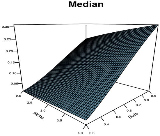
Figure 7. Median plot for the SAP-W.

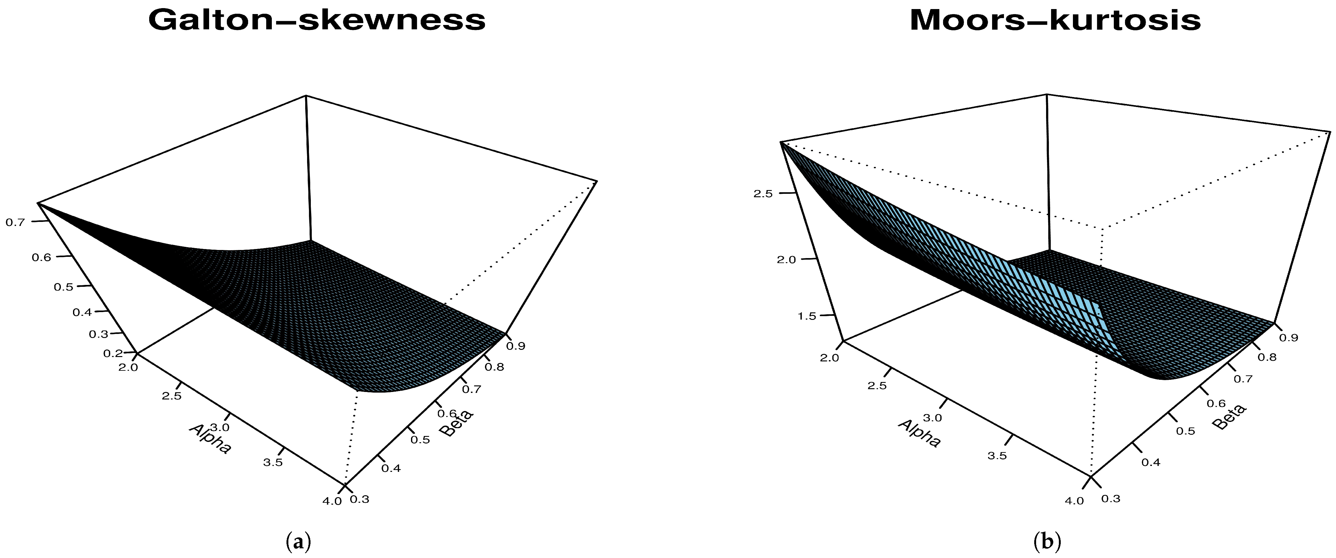
3.3. Skewness and Kurtosis

The forms of SAP-W may be investigated using Galton’s skewness and Moors’ kurtosis [27]. This is simply determined via (18), as below:

$$\mathrm{Skewness}={\displaystyle \frac{Q\left(\frac{3}{4}\right)-2Q\left(\frac{1}{2}\right)+Q\left(\frac{1}{4}\right)}{Q\left(\frac{3}{4}\right)-Q\left(\frac{1}{4}\right)}},$$

$$\mathrm{Kurtosis}={\displaystyle \frac{Q\left(\frac{7}{8}\right)-Q\left(\frac{5}{8}\right)-Q\left(\frac{1}{8}\right)+Q\left(\frac{3}{8}\right)}{Q\left(\frac{3}{4}\right)-Q\left(\frac{1}{4}\right)}}.$$

The plots in Figure 8 indicate that skewness and kurtosis decrease for the values considered of $\alpha$ and $\beta$.

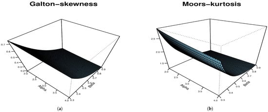
Figure 8. Skewness and kurtosis plots for SAP-W: (a) Galton skewness, (b) Moors kurtosis.

3.4. Moments

If X has SAP-W with PDF in (14), then the $rth$ moment of X is provided by

$${\mu }_r=E\left(x^r\right)={\int }_0^{\infty }{x}^{r}g\left(x\right)dx=\lambda \beta \sum _{j=0}^{\infty }{\psi }_j{\int }_0^{\infty }{x}^{r+\beta -1}{e}^{-(j+1)\lambda x^{\beta }}dx.$$

Let $u=(j+1)\lambda x^{\beta }$; we obtain

$${\mu }_r=\sum _{j=0}^{\infty }{\displaystyle \frac{{\psi }_j}{{\lambda }^{\frac{r}{\beta }}{(j+1)}^{\frac{r}{\beta }+1}}}{\int }_0^{\infty }{u}^{{\displaystyle \frac{r}{\beta }}}{e}^{-u}du.$$

Thus, the $rth$ moment is illustrated by

$${\mu }_r=\sum _{j=0}^{\infty }{\displaystyle \frac{{\psi }_j\Gamma (\frac{r}{\beta }+1)}{{\lambda }^{\frac{r}{\beta }}{(j+1)}^{\frac{r}{\beta }+1}}}.$$

(19)

Consequently, the SAP-W mean can simply be written as

$$\mu =E\left(x\right)=\sum _{j=0}^{\infty }{\displaystyle \frac{{\psi }_j\Gamma (\frac{1}{\beta }+1)}{{\lambda }^{\frac{1}{\beta }}{(j+1)}^{\frac{1}{\beta }+1}}}.$$

(20)

Furthermore, from (19) and (20) the variance for the SAP-W is given by

$$V\left(x\right)=E\left(x^2\right)-{\left[E\left(x\right)\right]}^2.$$

$$V\left(x\right)=\sum _{j=0}^{\infty }{\displaystyle \frac{{\psi }_j\Gamma (\frac{2}{\beta }+1)}{{\lambda }^{\frac{2}{\beta }}{(j+1)}^{\frac{2}{\beta }+1}}}-{\left(\sum _{j=0}^{\infty }{\displaystyle \frac{{\psi }_j\Gamma (\frac{1}{\beta }+1)}{{\lambda }^{\frac{1}{\beta }}{(j+1)}^{\frac{1}{\beta }+1}}}\right)}^2,$$

where ${\psi }_j$ is given by (15).

3.5. SAP-W Moment Generating and Characteristic Functions

The moment generating function, $M_x\left(t\right)$, and characteristic function, ${\varphi }_x\left(t\right)$, of SAP-W are, respectively, produced using the $rth$ moment of SAP-W as follows

$$M_x\left(t\right)=E\left(e^{tx}\right)=\sum _{r=0}^{\infty }{\displaystyle \frac{t^r}{r!}}{\mu }_r,$$

(21)

$${\varphi }_x\left(t\right)=E\left(e^{itx}\right)=\sum _{r=0}^{\infty }{\displaystyle \frac{{\left(itx\right)}^r}{r!}}.$$

(22)

Equation (19) can be substituted into (21) to obtain $M_x\left(t\right)$ of SAP-W

$$M_x\left(t\right)=\sum _{r=0}^{\infty }\sum _{j=0}^{\infty }{\displaystyle \frac{t^r}{r!}}{\displaystyle \frac{{\psi }_j\Gamma (\frac{r}{\beta }+1)}{{\lambda }^{\frac{r}{\beta }}{(j+1)}^{\frac{r}{\beta }+1}}}.$$

Similarly, ${\varphi }_x\left(t\right)$ of SAP-W is obtained as follows

$${\varphi }_x\left(t\right)=\sum _{r=0}^{\infty }\sum _{j=0}^{\infty }{\displaystyle \frac{{\left(it\right)}^r}{r!}}{\displaystyle \frac{{\psi }_j\Gamma (\frac{r}{\beta }+1)}{{\lambda }^{\frac{r}{\beta }}{(j+1)}^{\frac{r}{\beta }+1}}}.$$

3.6. Rényi Entropies

The Rényi entropy, $R{E}_X\left(v\right)$, for the SAP-W is given by

$$R{E}_X\left(v\right)={\displaystyle \frac{v}{1-v}}\left(log({\displaystyle \frac{\pi }{2}})+log(\alpha log\alpha )\right)-log\beta -{\displaystyle \frac{log\lambda }{\beta }}+{\displaystyle \frac{1}{1-v}}log\left({\displaystyle \frac{C\Gamma \left(\frac{v\beta -v+1}{\beta }\right)}{{(v+j)}^{\frac{v\beta -v+1}{\beta }}}}\right),$$

(23)

where

$$C=\sum _{k=0}^{\infty }\sum _{r=0}^k\sum _{i=0}^{\infty }\sum _{j=0}^{\infty }{(-1)}^{(v+r+i)}\left(\begin{array}{c}k\\ r\end{array}\right)\left(\begin{array}{c}r\\ i\end{array}\right){\displaystyle \frac{a_k{\alpha }^i{(-log\alpha )}^j{(v+i)}^j}{{(1-\alpha )}^{r+v}j!}}.$$

Proof. 

The Rényi entropy of a RV X is a measure of uncertainty variation. It is provided by

$$R{E}_X\left(v\right)={\displaystyle \frac{1}{1-v}}log\left({\int }_0^{\infty }{g}^v\left(x\right)dx\right),v>0,v\ne 1.$$

Using the SAP-W PDF in (11), the $R{E}_X\left(v\right)$ of X may be calculated as follows

$$R{E}_X\left(v\right)={\displaystyle \frac{1}{1-v}}log\left[{\left({\displaystyle \frac{\pi \lambda \beta \alpha log\alpha }{2(\alpha -1)}}\right)}^{v}J\right],x>0,\alpha ,\lambda ,\beta >0,\alpha \ne 1,$$

and $J={\int }_0^{\infty }{x}^{v(\beta -1)}{e}^{-v\lambda x^{\beta }}{\alpha }^{-v{e}^{-\lambda x^{\beta }}}{cos}^v\left[{\displaystyle \frac{\pi }{2}}{\displaystyle \frac{1-{\alpha }^{1-e^{-\lambda x^{\beta }}}}{1-\alpha }}\right]dx.$ By expanding $W\left(s\right)={cos}^v\left[{\displaystyle \frac{\pi }{2}}s\right]$ in the Taylor series [11], expressed as

$${cos}^v\left[{\displaystyle \frac{\pi }{2}}s\right]=\sum _{k=0}^{\infty }\sum _{r=0}^k{(-1)}^r{a}_k\left(\begin{array}{c}k\\ r\end{array}\right)s^r,$$

where $a_k={\displaystyle \frac{{(-1)}^k{W}^{\left(k\right)}\left(1\right)}{k!}}$, and $W^{\left(k\right)}\left(1\right)$ denotes the $k^{th}$ derivative of W(.) evaluated at the point 1. Then applying the series in (16), $R{E}_X\left(v\right)$ will reduce to

$$R{E}_X\left(v\right)={\displaystyle \frac{1}{1-v}}log\left[{\left({\displaystyle \frac{\pi \lambda \beta \alpha log\alpha }{2(\alpha -1)}}\right)}^v\sum _{k=0}^{\infty }\sum _{r=0}^k\sum _{i=0}^{\infty }{(-1)}^{r+i}I\right],$$

where $I=\left(\begin{array}{c}k\\ r\end{array}\right)\left(\begin{array}{c}r\\ i\end{array}\right){\displaystyle \frac{a_k{\alpha }^i}{{(1-\alpha )}^r}}{\int }_0^{\infty }{x}^{v(\beta -1)}{e}^{-v\lambda x^{\beta }}{\alpha }^{-(v+i)e^{-\lambda x^{\beta }}}dx.$ By applying the series form in (17) and the transformation $y=(v+j)\lambda x^{\beta }$, we obtain (23). □

3.7. Order Statistics

Assume that $X_{i:m}$ is the ith order statistics and that $X_1,X_2,\dots ,X_m$ is a random sample taken from SAP-W. Consequently, the expression of the PDF of the ith order statistics, $g_{i:m}\left(x\right)$, is

$$g_{i:m}\left(x\right)={\displaystyle \frac{m!}{(i-1)!(m-i)!}}g\left(x\right){\left[G\left(x\right)\right]}^{i-1}{[1-G\left(x\right)]}^{m-i},$$

where $g\left(x\right)$ and $G\left(x\right)$ are the PDF and CDF of SAP-W defined in (11) and (10), respectively.

The PDF of $X_{i:m}$ may be stated as

$$\begin{array}{l}{g}_{i:m}\left(x\right)={\displaystyle \frac{1}{B(i,m-i+1)}}g\left(x\right){\left[sin\left[{\displaystyle \frac{\pi }{2}}\left({\displaystyle \frac{1-{\alpha }^{1-e^{-\lambda x^{\beta }}}}{1-\alpha }}\right)\right]\right]}^{i-1}\\ \times {\left[1-sin\left[{\displaystyle \frac{\pi }{2}}\left({\displaystyle \frac{1-{\alpha }^{1-e^{-\lambda x^{\beta }}}}{1-\alpha }}\right)\right]\right]}^{m-i},x,\alpha ,\lambda ,\beta >0,\alpha \ne 1.\end{array}$$

(24)

where $B(i,m-i+1)$ refers to the beta function. Specifically, assuming $i=1$, we obtain the PDF of the first-order statistics defined by

$$g_{1:m}\left(x\right)={\displaystyle \frac{1}{B(1,m)}}g\left(x\right){\left[1-sin\left[{\displaystyle \frac{\pi }{2}}\left({\displaystyle \frac{1-{\alpha }^{1-e^{-\lambda x^{\beta }}}}{1-\alpha }}\right)\right]\right]}^{m-1}.$$

In addition, the PDF of the largest order statistic is obtained by assuming $i=m$.

$$g_{m:m}\left(x\right)={\displaystyle \frac{1}{B(m,1)}}g\left(x\right){\left[sin\left[{\displaystyle \frac{\pi }{2}}\left({\displaystyle \frac{1-{\alpha }^{1-e^{-\lambda x^{\beta }}}}{1-\alpha }}\right)\right]\right]}^{m-1}.$$

4. Parameter Estimation

Suppose we selected a random sample of size n from the SAP-W; then, the log-likelihood $(\mathsf{\ell })$ for the parameters vector, $\Phi =(\alpha ,\lambda ,\beta )$, is

$$\begin{array}{c}\mathsf{\ell }(\Phi ;x)=nlog\left({\displaystyle \frac{\pi }{2}}\right)+nlog\left({\displaystyle \frac{log\alpha }{\alpha -1}}\right)+nlog\left(\alpha \lambda \beta \right)+(\beta -1)\sum _{i=1}^{n}log{x}_i\hfill \\ -log\alpha \sum _{i=1}^n{e}^{-\lambda x_i^{\beta }}-\lambda \sum _{i=1}^n{x}_i^{\beta }+\sum _{i=1}^{n}log\left(cos\left[{\displaystyle \frac{\pi }{2}}\left({\displaystyle \frac{1-{\alpha }^{1-e^{-\lambda x_i^{\beta }}}}{1-\alpha }}\right)\right]\right).\end{array}$$

(25)

The first derivatives of the log-likelihood equation with respect to $\lambda$, $\alpha$, and $\beta$ are provided as follows

$$\begin{array}{c}{\displaystyle \frac{\partial \mathsf{\ell }}{\partial \lambda }}={\displaystyle \frac{n}{\lambda }}-\sum _{i=1}^n{x}_i^{\beta }+log\alpha \sum _{i=1}^n{x}_i^{\beta }{e}^{-\lambda x_i^{\beta }}+{\displaystyle \frac{\pi log\alpha }{2(1-\alpha )}}\hfill \\ \times \sum _{i=1}^n{\alpha }^{1-e^{-\lambda x_i^{\beta }}}{e}^{-\lambda x_i^{\beta }}{x}_i^{\beta }\left(tan\left[{\displaystyle \frac{\pi }{2}}\left({\displaystyle \frac{1-{\alpha }^{1-e^{-\lambda x_i^{\beta }}}}{1-\alpha }}\right)\right]\right),\end{array}$$

(26)

$$\begin{array}{c}{\displaystyle \frac{\partial \mathsf{\ell }}{\partial \alpha }}={\displaystyle \frac{n}{\alpha }}-{\displaystyle \frac{{\sum }_{i=1}^n{e}^{-\lambda x_i^{\beta }}}{\alpha }}+{\displaystyle \frac{n(\alpha -1-\alpha log\alpha )}{\alpha (\alpha -1)log\alpha }}\hfill \\ -\sum _{i=1}^n\left(tan\left[{\displaystyle \frac{\pi }{2}}\left({\displaystyle \frac{1-{\alpha }^{1-e^{-\lambda x_i^{\beta }}}}{1-\alpha }}\right)\right]\right)\left({\displaystyle \frac{\pi (1-{\alpha }^{1-e^{-\lambda x_i^{\beta }}})}{2{(1-\alpha )}^2}}-{\displaystyle \frac{\pi {\alpha }^{-e^{-\lambda x_i^{\beta }}}(1-e^{-\lambda x_i^{\beta }})}{2(1-\alpha )}}\right),\end{array}$$

(27)

$$\begin{array}{c}{\displaystyle \frac{\partial \mathsf{\ell }}{\partial \beta }}={\displaystyle \frac{n}{\beta }}+\lambda log\alpha \sum _{i=1}^n{x}_i^{\beta }{e}^{-\lambda x_i^{\beta }}log{x}_i-\lambda \sum _{i=1}^n{x}_i^{\beta }log{x}_i+\sum _{i=1}^{n}log{x}_i\hfill \\ +{\displaystyle \frac{\pi \lambda log\alpha }{2(1-\alpha )}}\sum _{i=1}^n{\alpha }^{1-e^{-\lambda x_i^{\beta }}}{e}^{-\lambda x_i^{\beta }}{x}_i^{\beta }log{x}_i\left(tan\left[{\displaystyle \frac{\pi }{2}}\left({\displaystyle \frac{1-{\alpha }^{1-e^{-\lambda x_i^{\beta }}}}{1-\alpha }}\right)\right]\right).\end{array}$$

(28)

The maximum likelihood estimates (MLEs) of the unknown parameters can be obtained by solving the nonlinear equations in (26)–(28) numerically or directly by maximizing (25), using some optimization techniques such as the Newton–Raphson method in the R package. The MLEs have an asymptotically normal distribution; that is, $\sqrt{n}(\widehat{\alpha }-\alpha ,\widehat{\lambda }-\lambda ,\widehat{\beta }-\beta )\sim N_3(0,\Sigma )$, where $\Sigma$ represents the variance-covariance matrix and can be produced via inverting the observed Fisher information matrix F, as below: $F=\left[\begin{array}{ccc}{\displaystyle \frac{{\partial }^{2}log\mathsf{\ell }}{\partial {\alpha }^2}}& {\displaystyle \frac{{\partial }^{2}log\mathsf{\ell }}{\partial \alpha \partial \lambda }}& {\displaystyle \frac{{\partial }^{2}log\mathsf{\ell }}{\partial \alpha \partial \beta }}\\ {\displaystyle \frac{{\partial }^{2}log\mathsf{\ell }}{\partial \lambda \partial \alpha }}& {\displaystyle \frac{{\partial }^{2}log\mathsf{\ell }}{\partial {\lambda }^2}}& {\displaystyle \frac{{\partial }^{2}log\mathsf{\ell }}{\partial \lambda \partial \beta }}\\ {\displaystyle \frac{{\partial }^{2}log\mathsf{\ell }}{\partial \beta \partial \alpha }}& {\displaystyle \frac{{\partial }^{2}log\mathsf{\ell }}{\partial \beta \partial \lambda }}& {\displaystyle \frac{{\partial }^{2}log\mathsf{\ell }}{\partial {\beta }^2}}\end{array}\right].$

5. Simulation Study

We performed Monte Carlo simulations to examine how the MLEs of the SAP-W parameters will behave for various sample sizes and parameter values. (18) was applied to generate 1000 random samples with size $n=15,25,50,100,$ and $200.$ The following four sets of parameters were used:

$$\mathrm{Set}\mathrm{I}:\alpha =1.5,\lambda =2,\beta =1.2,$$

$$\mathrm{Set}\mathrm{II}:\alpha =1.5,\lambda =2.5,\beta =1.5,$$

$$\mathrm{Set}\mathrm{III}:\alpha =1.3,\lambda =1.9,\beta =0.9.$$

$$\mathrm{Set}\mathrm{IV}:\alpha =0.03,\lambda =1,\beta =0.5.$$

The estimates of the parameters were produced for each sample size, and their mean square error (MSE) was computed and obtained from

$${MSE}_{\Phi }={\displaystyle \frac{1}{1000}}\sum _{i=1}^{1000}{({\widehat{\Phi }}_i-\Phi )}^2,$$

where $\Phi =(\alpha ,\lambda ,\beta )$. Based on the results in Table 1, the MLEs of the parameters for the SAP-W distribution approach their actual values. Moreover, the analysis of MSE in parameter estimation shows that the accuracy of the estimate improves as the sample size increases. When $\alpha >1$ in Sets I, II, and III, the MSE is relatively high for small sample sizes but drops significantly once the sample size reaches 100 or more, confirming the asymptotic efficiency of the estimators. Moreover, in Set IV, when $\alpha <1$, the results indicate that the MSE remains relatively low even for small sample sizes, indicating that the distribution remains significantly stable under these conditions.

Table 1. The SAP-W simulation outcomes.

		Set I		Set II		Set III		Set IV
	Parameter	MLEs	MSE	MLEs	MSE	MLEs	MSE	MLEs	MSE
n = 15	$\alpha$	12.3790	118.3521	11.7114	104.2730	12.1073	116.7967	0.0022	0.0008
	$\lambda$	3.9083	3.6416	5.0854	6.6844	3.8257	3.7082	1.1634	0.0267
	$\beta$	1.4036	0.0414	1.7717	0.0738	1.0395	0.0195	0.7478	0.0614
n = 25	$\alpha$	10.8435	87.3019	10.8927	88.2224	10.5554	85.6629	0.0014	0.0008
	$\lambda$	2.9422	0.8877	3.5750	1.1557	2.8931	0.9862	0.5792	0.1770
	$\beta$	1.0462	0.0237	1.3069	0.0373	0.7766	0.0152	0.5390	0.0015
n = 50	$\alpha$	5.3361	14.7160	5.3192	14.5862	5.1764	15.0266	0.0016	0.0008
	$\lambda$	2.7141	0.5100	3.3378	0.7019	2.6624	0.5813	0.5919	0.1665
	$\beta$	1.1140	0.0074	1.3931	0.0114	0.8274	0.0053	0.5287	0.0008
n = 100	$\alpha$	1.6996	0.0398	1.7004	0.0402	1.6076	0.0946	0.0038	0.0007
	$\lambda$	2.4340	0.1883	3.0867	0.3442	2.3648	0.2160	0.7599	0.0576
	$\beta$	1.2773	0.0060	1.5966	0.0093	0.9503	0.0025	0.5260	0.0007
n = 200	$\alpha$	1.5326	0.0011	1.5314	0.0010	1.3209	0.0004	0.0232	0.0001
	$\lambda$	1.9429	0.0033	2.4410	0.0035	1.8410	0.0035	0.9034	0.0093
	$\beta$	1.2281	0.0008	1.5354	0.0012	0.9213	0.0005	0.5100	0.0001

6. Applications

In this section, we present three real-life engineering datasets to demonstrate the versatility of the SAP-W.

• Data 1: Breaking stress of carbon fibers.
• These real data are obtained from [28] and include 100 observations. The data are as follows:
• 3.7, 2.74, 2.73, 2.5, 3.6, 3.11, 3.27, 2.87, 1.47, 3.11, 4.42, 2.41, 3.19, 3.22, 1.69, 3.28, 3.09, 1.87, 3.15, 4.9, 3.75, 2.43, 2.95, 2.97, 3.39, 2.96, 2.53, 2.67, 2.93, 3.22, 3.39, 2.81, 4.2, 3.33, 2.55, 3.31, 3.31, 2.85, 2.56, 3.56, 3.15, 2.35, 2.55, 2.59, 2.38, 2.81, 2.77, 2.17, 2.83, 1.92, 1.41, 3.68, 2.97, 1.36, 0.98, 2.76, 4.91, 3.68, 1.84, 1.59, 3.19, 1.57, 0.81, 5.56, 1.73, 1.59, 2, 1.22, 1.12, 1.71, 2.17, 1.17, 5.08, 2.48, 1.18, 3.51, 2.17, 1.69, 1.25, 4.38, 1.84, 0.39, 3.68, 2.48, 0.85, 1.61, 2.79, 4.7, 2.03, 1.8, 1.57, 1.08, 2.03, 1.61, 2.12, 1.89, 2.88, 2.82, 2.05, 3.65.
• Data 2: Electrical Appliance Failure Data.
• These data are provided by [29] and refer to the number of 1000s of cycles of failure for electrical appliances in a life test, given as follows:
• 0.014, 0.034, 0.059, 0.061, 0.069, 0.080, 0.123, 0.142, 0.165, 0.210, 0.381, 0.464, 0.479, 0.556, 0.574, 0.839, 0.917, 0.969, 0.991, 1.064, 1.088, 1.091, 1.174, 1.270, 1.275, 1.355, 1.397, 1.477, 1.578, 1.649, 1.702, 1.893, 1.932, 2.001, 2.161, 2.292, 2.326, 2.337, 2.628, 2.785, 2.811, 2.886, 2.993, 3.122, 3.248,3.715, 3.790, 3.857, 3.912, 4.100, 4.106, 4.116, 4.315, 4.510, 4.580, 5.267, 5.299, 5.583, 6.065, 9.701.
• Data 3: Aircraft windshields.
• These data present the service times of 63 aircraft windshields measured in 1000 h, given in [30]. The data are as follows:
• 0.046, 1.436, 2.592, 0.140, 1.492, 2.600, 0.150, 1.580, 2.670, 0.248, 1.719, 2.717, 0.280, 1.794, 2.819, 0.313, 1.915, 2.820, 0.389, 1.920, 2.878, 0.487, 1.963, 2.950, 0.622, 1.978, 3.003, 0.900, 2.053, 3.102, 0.952, 2.065, 3.304, 0.996, 2.117, 3.483, 1.003, 2.137, 3.500, 1.010, 2.141, 3.622, 1.085, 2.163, 3.665, 1.092, 2.183, 3.695, 1.152, 2.240, 4.015, 1.183, 2.341, 4.628, 1.244, 2.435, 4.806, 1.249, 2.464, 4.881, 1.262, 2.543, 5.140.

Table 2 shows several statistical measurements for the three sets of data.

Table 2. Summary statistics for the three datasets.

Data	Size	Mean	Median	Min.	Max.	First Quartile	Third Quartile
1	100	2.621	2.700	0.390	5.560	1.840	3.220
2	60	2.193	1.676	0.014	9.701	0.773	3.365
3	63	2.085	2.065	0.046	5.140	1.122	2.820

The SAP-W is compared to five other competing distributions with the following CDF:

• Gull alpha power Weibull (GAPW) distribution in [31]:

  $$F\left(y\right)={\displaystyle \frac{\alpha (1-e^{-\beta y^{\gamma }})}{{\alpha }^{1-e^{-\beta y^{\gamma }}}}},y>0,\alpha ,\gamma ,\beta >0.$$
• A new alpha power transformed Weibull (NAPW) distribution in [32]:

  $$F\left(x\right)={\displaystyle \frac{(1-e^{-\gamma x^{\theta }}){\alpha }^{(1-e^{-\gamma x^{\theta }})}}{\alpha }},x>0,\alpha ,\gamma ,\theta >0.$$
• Alpha power Weibull (APW) distribution in [4]:

  $$F\left(x\right)=\left\{\begin{array}{ccc}\hfill {\displaystyle \frac{1}{1-\alpha }}(1-{\alpha }^{1-e^{-\lambda x^{\beta }}})& \mathrm{i}\mathrm{f}& \alpha >0,\alpha \ne 1,\hfill \\ \hfill 1-e^{-\lambda x^{\beta }}& \mathrm{i}\mathrm{f}& \alpha =1,\hfill \end{array}\right.$$

  where $x>0,\lambda ,\beta >0$.
• Sine inverse Weibull (SIW) distribution in [11]:

  $$F\left(x\right)=sin\left[{\displaystyle \frac{\pi }{2}}{e}^{-\alpha x^{-\theta }}\right],x>0,\alpha ,\theta >0.$$
• Sine inverse exponential (SIE) distribution in [33]:

  $$F\left(x\right)=sin\left[{\displaystyle \frac{\pi }{2}}{e}^{-(\theta /x)}\right],x>0,\theta >0.$$

To determine the validity of the suggested model compared to other models, we calculated some GoF criteria: the negative log-likelihood ($-\widehat{\mathsf{\ell }}$), Akaike information criterion (AIC), Bayesian information criterion (BIC), consistent Akaike information criterion (CAIC), and the Kolmogorov–Smirnov (KS) test with its p-value. The formula for these metrics are supplied by

$$\begin{array}{c}\hfill AIC=2k-2\widehat{\mathsf{\ell }}.\\ \hfill BIC=klog\left(n\right)-2\widehat{\mathsf{\ell }}.\\ \hfill CAIC={\displaystyle \frac{2kn}{n-k-1}}-2\widehat{\mathsf{\ell }}.\end{array}$$

where $\widehat{\mathsf{\ell }}$ denotes the maximized log-likelihood function, k represents the number of estimated parameters in the model, and n is the number of observations. The lower values of $-\widehat{\mathsf{\ell }}$, AIC, BIC, CAIC, and KS, and higher p-value indicate better fits.

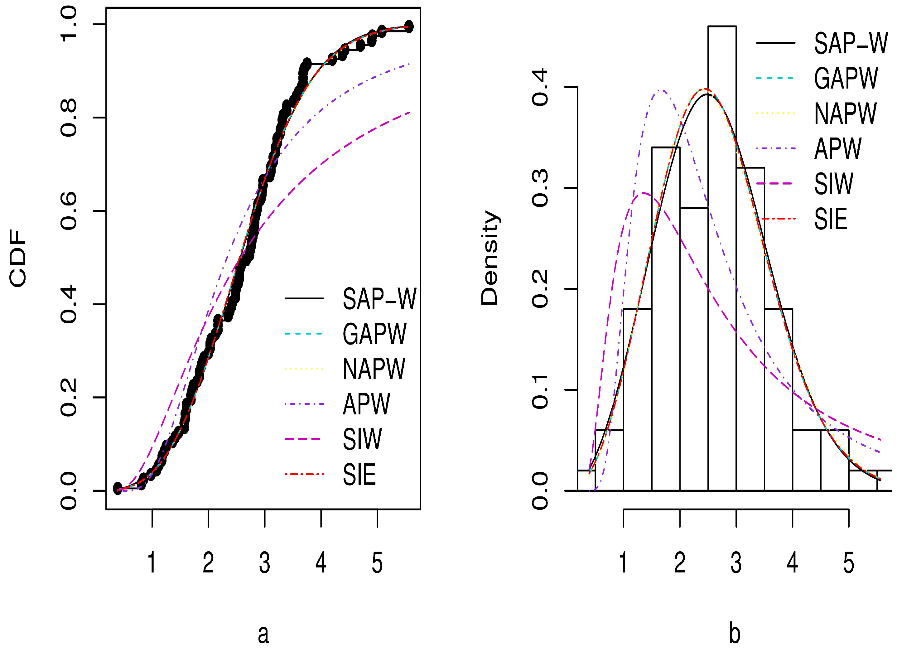
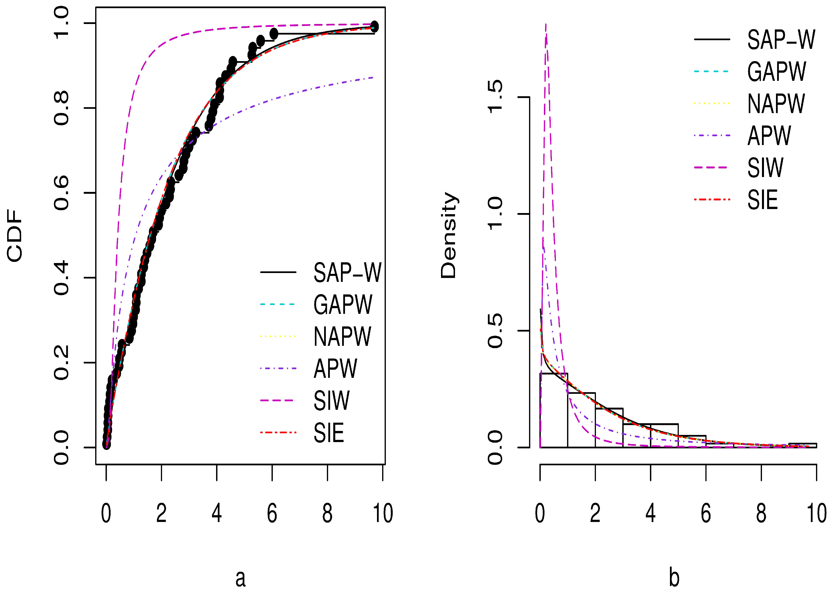
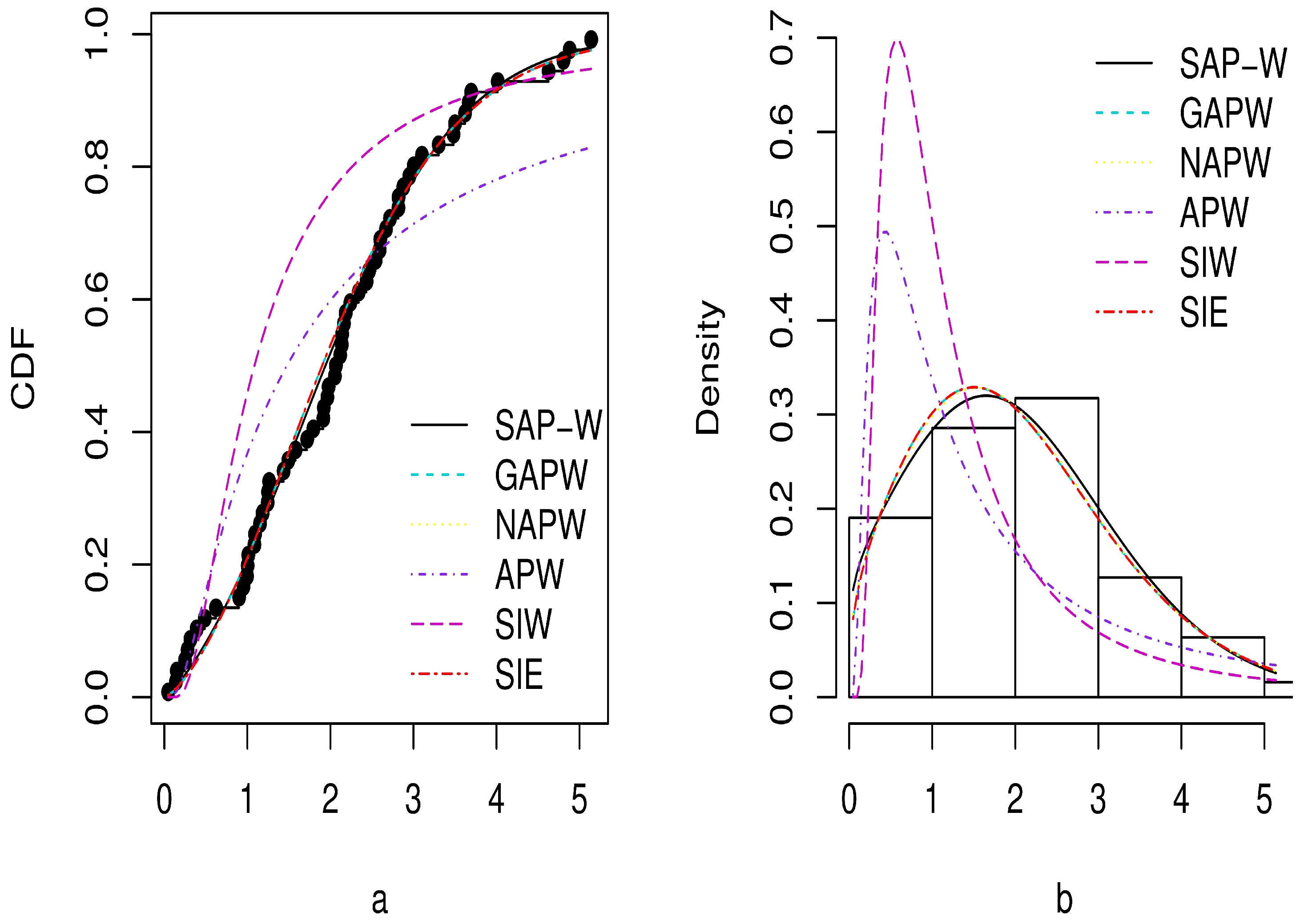
The MLEs, standard errors (SE), and GoF criteria for the SAP-W, GAPW, NAPW, APW, SIW, and SIE distributions are reported in Table 3, Table 4, Table 5 and Table 6 for the three datasets. According to the outcomes in Table 4, Table 5 and Table 6, the SAP-W gives a superior fit with the minimum values $-\widehat{\mathsf{\ell }}$, AIC, BIC, CAIC, KS, and greatest p-values when compared to the other competing distributions considered in this study. In addition, Figure 9, Figure 10 and Figure 11 display the density and CDF for the SAP-W and the competitive distributions. The histogram represents the empirical density for the data, and the black dots represent the empirical CDF for the data. The figures indicate that SAP-W most closely and accurately matches the actual distribution of the three analyzed datasets. Consequently, the SAP-W is the most suitable model for the investigated data when compared to competing distributions.

Table 3. MLEs and SE for the three datasets.

Distribution	Parameter		MLEs and SE in ()
		Data 1	Data 2	Data 3
SAP-W	$\alpha$	0.2030 (0.3808)	6.0303 (7.7353 )	10.0078 (14.3150)
	$\lambda$	0.0140 (0.0111)	0.5347 (0.2505)	0.4196 (0.2354)
	$\beta$	2.8962 (0.2389)	0.7882 (0.1644)	1.1880 (0.2745)
GAPW	$\alpha$	2.1148 (0.8315)	0.5427 (0.3674)	0.4108 (0.3250)
	$\gamma$	3.1049 (0.2437)	0.8906 (0.1539 )	1.3714 (0.2527)
	$\beta$	0.0190 (0.0091)	0.6539 (0.2433)	0.4602 (0.2085)
NAPW	$\alpha$	0.4749 (0.1889)	1.8425 (1.2472)	2.4342 (1.9259)
	$\gamma$	0.0191 (0.0093)	0.6538 (0.2433)	0.4602 (0.2085)
	$\theta$	3.1050 (0.2426)	0.8906 (0.1539)	1.3713 (0.2527)
APW	$\alpha$	0.1687 (0.3910)	3.6821 (4.3293)	5.9036 (7.4776)
	$\lambda$	0.0182 (0.0195)	0.7011 (0.2734)	0.5054 (0.2356)
	$\beta$	3.1896 (0.3659)	0.8702 (0.1581)	1.3327 (0.2567)
SIW	$\alpha$	3.7887 (0.3477)	1.1300 (0.1159)	1.4278 (0.1364)
	$\theta$	1.4625 (0.0930)	0.4646 (0.0397)	0.6732 (0.0537)
SIE	$\theta$	2.8243 (0.2151)	0.4577 (0.0435)	1.1914 (0.1108)

Table 4. GoF measures for Dataset 1.

Distribution	$-\widehat{\mathit{\ell }}$	AIC	BIC	CAIC	K-S	p-Values
SAP-W	141.1779	288.3559	296.1714	292.2636	0.0634	0.8165
GAPW	141.1785	288.3569	296.1724	292.2647	0.0686	0.7340
NAPW	141.1788	288.3576	296.1731	292.2654	0.0687	0.7320
APW	141.3403	288.6807	296.4962	292.5884	0.0697	0.7159
SIW	161.5795	327.159	332.3694	329.7642	0.1358	0.0501
SIE	174.6757	351.3514	353.9566	352.6540	0.2460	1.113 × ${10}^{-5}$

Table 5. GoF measures for Dataset 2.

Distribution	$-\widehat{\mathit{\ell }}$	AIC	BIC	CAIC	K-S	p-Values
SAP-W	105.9299	217.8598	224.1428	221.0013	0.0741	0.8723
GAPW	106.6183	219.2366	225.5197	222.3782	0.0779	0.8315
NAPW	106.6183	219.2366	225.5197	222.3782	0.0779	0.8315
APW	106.5183	219.0365	225.3195	222.1780	0.0777	0.8343
SIW	123.7684	251.5369	255.7256	253.6312	0.1990	0.0147
SIE	200.5836	403.1671	405.2615	404.2143	0.5488	6.661 × ${10}^{-16}$

Table 6. GoF measures for Dataset 3.

Distribution	$-\widehat{\mathit{\ell }}$	AIC	BIC	CAIC	K-S	p-Values
SAP-W	98.77106	203.5421	209.9715	206.7568	0.0796	0.7894
GAPW	99.5222	205.0444	211.4738	208.2591	0.0920	0.6275
NAPW	99.5222	205.0444	211.4738	208.2591	0.0920	0.6274
APW	99.3842	204.7685	211.1979	207.9832	0.0891	0.6655
SIW	123.2494	250.4987	254.7850	252.6419	0.1927	0.0160
SIE	141.3209	284.6417	286.7848	285.7133	0.3341	9.019 × ${10}^{-7}$

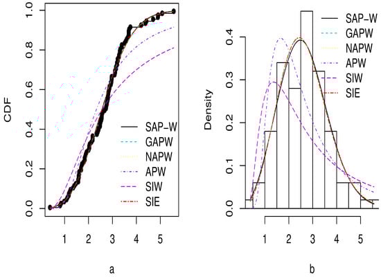
Figure 9. Plots of estimated CDF in (a) and PDF in (b) for Dataset 1.

Figure 10. Plots of estimated CDF in (a) and PDF in (b) for Dataset 2.

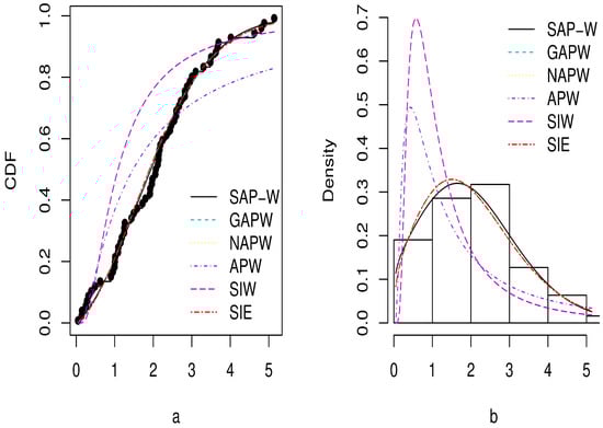
Figure 11. Plots of estimated CDF in (a) and PDF in (b) for Dataset 3.

Furthermore, the SAP-W model demonstrates significant advantages in various industries due to its flexibility and ability to model complex failure patterns. In the fields of manufacturing and material science, the SAP-W model plays a crucial role. It accurately models the breaking stress of carbon fibers, capturing varying failure rates due to material properties and external factors. In the electronics and appliances industry, the SAP-W handles different failure behaviors (early-life, random, wear-out) in appliances, improving maintenance scheduling and product reliability. In aerospace and aviation, the SAP-W’s ability to model failure rates that are not monotonic helps predict how long important parts, such as airplane windshields, will last, which improves safety and maintenance planning.

7. The Log SAP-W Regression Model

In this section, the log SAP-W (LSAP-W) regression model is introduced. Applying the transformation $Y=log\left(X\right)$ in (11) and taking the re-parametrization $\beta ={\displaystyle \frac{1}{\sigma }}$, $\lambda =e^{{\displaystyle \frac{-\mu }{\sigma }}}$ into consideration will produce the LSAP-W. Then, the PDF of LSAP-W can be expressed as

$$g\left(y\right)={\displaystyle \frac{\pi }{2}}{\displaystyle \frac{log\alpha }{(\alpha -1)\sigma }}exp\left[{\displaystyle \frac{y-\mu }{\sigma }}-exp\left({\displaystyle \frac{y-\mu }{\sigma }}\right)\right]{\alpha }^{1-exp\left[-exp\left({\displaystyle \frac{y-\mu }{\sigma }}\right)\right]}cos\left[{\displaystyle \frac{\pi }{2}}\left({\displaystyle \frac{1-{\alpha }^{1-exp\left[-exp\left(\frac{y-\mu }{\sigma }\right)\right]}}{1-\alpha }}\right)\right],$$

(29)

where $\mu \in \mathbb{R}$ is the location parameter, $\sigma >0$ is the scale parameter, and $\alpha >0,\alpha \ne 1.$

The corresponding CDF is presented as

$$G\left(y\right)=sin\left[{\displaystyle \frac{\pi }{2}}\left({\displaystyle \frac{1-{\alpha }^{1-exp\left[-exp\left(\frac{y-\mu }{\sigma }\right)\right]}}{1-\alpha }}\right)\right].$$

(30)

The survival $s\left(y\right)$ and hazard $h\left(y\right)$ functions are, respectively, as follows:

$$s\left(y\right)=1-sin\left[{\displaystyle \frac{\pi }{2}}\left({\displaystyle \frac{1-{\alpha }^{1-exp\left[-exp\left(\frac{y-\mu }{\sigma }\right)\right]}}{1-\alpha }}\right)\right],$$

(31)

$$h\left(y\right)={\displaystyle \frac{\pi }{2}}{\displaystyle \frac{log\alpha }{(\alpha -1)\sigma }}exp\left[{\displaystyle \frac{y-\mu }{\sigma }}-exp\left({\displaystyle \frac{y-\mu }{\sigma }}\right)\right]{\alpha }^{1-exp\left[-exp\left({\displaystyle \frac{y-\mu }{\sigma }}\right)\right]}{\displaystyle \frac{cos\left[\frac{\pi }{2}\left(\frac{1-{\alpha }^{1-exp\left[-exp\left(\frac{y-\mu }{\sigma }\right)\right]}}{1-\alpha }\right)\right]}{1-sin\left[\frac{\pi }{2}\left(\frac{1-{\alpha }^{1-exp\left[-exp\left(\frac{y-\mu }{\sigma }\right)\right]}}{1-\alpha }\right)\right]}}.$$

The quantile function is

$$Q\left(u\right)=\sigma ln\left[ln\left({\displaystyle \frac{ln\alpha }{ln\left(\left(\pi \alpha \right)/(\pi +2(\alpha -1)arcsinu))\right)}}\right)\right]+\mu .$$

In (29), the standardized RV for y is given as $z={\displaystyle \frac{y-\mu }{\sigma }}$, and z has the following PDF:

$$g\left(z\right)={\displaystyle \frac{\pi }{2}}{\displaystyle \frac{log\alpha }{(\alpha -1)}}exp\left[z-exp\left(z\right)\right]{\alpha }^{1-exp\left[-exp\left(z\right)\right]}cos\left[{\displaystyle \frac{\pi }{2}}\left({\displaystyle \frac{1-{\alpha }^{1-exp\left[-exp\left(z\right)\right]}}{1-\alpha }}\right)\right],$$

(32)

with the survival function given as

$$s\left(z\right)=1-sin\left[{\displaystyle \frac{\pi }{2}}\left({\displaystyle \frac{1-{\alpha }^{1-exp\left[-exp\left(z\right)\right]}}{1-\alpha }}\right)\right].$$

(33)

In several real-world scenarios, explanatory factors like blood pressure, cholesterol, weight, and others have an impact on life expectancy. There are several types of regression models used in survival analysis. Log-location-scale regression is one of the popular models commonly used by statisticians to estimate univariate survival functions for censored data [29]. Numerous studies have proposed applying log-location-scale regression models based on continuous distributions in several disciplines [34,35,36,37]. In general, a parametric model that fits the data well produces more accurate estimates of the quantities of interest. Therefore, we introduce a novel linear location-scale regression model based on the LSAP-W that links the response variable $y_i$ and the explanatory vector $x_i^T$ as follows:

$$y_i=\beta x_i^T+\sigma z_i,i=1,2,..,n,$$

(34)

where $z_i$ is the random error with PDF in (32), $\beta ={({\beta }_1,..,{\beta }_p)}^T,\alpha ,\sigma >0$ are the unknown parameters, and the explanatory vector is $x_i^T={(x_{i1},...,x_{ip})}^T$. The location of $y_i$ is represented by the parameter ${\mu }_i=\beta x_i^T$, and the location parameter vector $\mu ={({\mu }_1,...,{\mu }_n)}^T$ may be expressed as a linear model $\mu =\beta x$, where $x={(x_1,...,x_n)}^T$ is the known model matrix.

7.1. Maximum Likelihood Estimation of the LSAP-W Regression Model

The parameters of the LSAP-W regression model are estimated by applying the maximum likelihood method. Assume that $(y_1,{\tau }_1,x_1),\dots ,(y_n,{\tau }_n,x_n)$ represents a random sample of n observations for the right-censored lifetime data, with

$$y_i=\left\{\begin{array}{ccc}\hfill log\left(x_i\right)& \mathrm{i}\mathrm{f}& {\tau }_i=1\hfill \\ \hfill log\left(c_i\right)& \mathrm{i}\mathrm{f}& {\tau }_i=0\hfill \end{array}\right.,$$

where $x_i$ and $c_i$ are lifetimes and censoring times, respectively, which are independent and random. After that, for the parameter vector $\Theta =(\alpha ,\sigma ,{\beta }^T)$, the likelihood function $L(\Theta )$ is provided as follows:

$$L(\Theta )=\prod _{i=1}^n\left[g{\left(y_i\right)}^{{\tau }_i}s{\left(y_i\right)}^{1-{\tau }_i}\right],$$

(35)

so it is possible to derive the log-likelihood function,

$$logL\left(\theta \right)=\sum _{i=1}^n\left[{\tau }_{i}log{\displaystyle \frac{1}{\sigma }}+{\tau }_{i}logg\left(z_i\right)+(1-{\tau }_i)logs\left(z_i\right)\right],$$

(36)

whereas $g\left(z_i\right)$ represents the PDF in (32) and $s\left(z_i\right)$ represents the survival function in (33). Thus, we have

$$\begin{array}{c}logL(\Theta )=rlog(\pi log\left(\alpha \right))-rlog\left(2(\alpha -1)\right)-rlog\left(\sigma \right)+\sum _{i=1}^n{\tau }_i\left[z_i-exp\left(z_i\right)\right]+\sum _{i=1}^n{\tau }_i\left[1-exp[-exp\left(z_i\right)]\right]log\left(\alpha \right)\hfill \\ +\sum _{i=1}^n{\tau }_{i}log\left[cos\left[{\displaystyle \frac{\pi }{2}}\left({\displaystyle \frac{1-{\alpha }^{1-exp\left[-exp\left(z_i\right)\right]}}{1-\alpha }}\right)\right]\right]+\sum _{i=1}^n(1-{\tau }_i)log\left[1-sin\left[{\displaystyle \frac{\pi }{2}}\left({\displaystyle \frac{1-{\alpha }^{1-exp\left[-exp\left(z_i\right)\right]}}{1-\alpha }}\right)\right]\right],\end{array}$$

(37)

where $z_i=(y_i-\beta x_i^T)/\sigma$ and r is the number of uncensored observations. By maximizing the log-likelihood function in (37), we can obtain the MLEs of the parameters. The MLEs might be produced using the “optim” function in the R package.

7.2. Applications for the LSAP-W Regression Model

We examine the performance of the LSAP-W regression model by using a real dataset and comparing it with various competing models. The dataset is known as the Leukemia Data and presented in [29]. This dataset includes information about 33 patients. Three variables are included in this dataset: the survival time in weeks, along with two explanatory variables; the white blood cell count (WBC) at diagnosis; and the white blood cell characteristics test (AG), divided into positive test results (AG = 1) and negative test results (AG = 0). The variables present are listed below:

• $t_i$, survival time;
• $y_i$, log survival time;
• status_i, censoring indication (0 = censoring, 1 = lifetime);
• $x_{i1}$, white blood cell characteristics test (0 = negative, 1 = positive);
• $x_{i2}$, white blood cell count.

Thus, the fitted model can be expressed as follows:

$$y_i={\beta }_0+{\beta }_1{x}_{i1}+{\beta }_2{x}_{i2}+\sigma z_i,i=1,2,...,33.$$

(38)

Table 7 displays the MLEs and their SE. We compare the LSAP-W regression model with the log cosine Topp–Leon Weibull (LCTLW) in [9], the log odds exponential-Pareto IV (LOEPIV) in [36], and the log Marshall–Olkin odd log-logistic Weibull (LMOOLLW) in [37], using the following criteria: the AIC, CAIC, BIC, and the Hannan–Quinn information criterion (HQC). The results in Table 8 indicate that the LSAP-W best fits the Leukemia Data as it has the lowest values of all GoF criteria compared to the other competitor models. In all fitted models, we observe that the coefficients for the variables AG and WBC are positive and negative, respectively. The parameter estimations indicated that when the AG test is positive and the WBC is low at diagnosis, the survival time for leukemic patients increases.

Table 7. MLEs, SE in () for the Leukemia Data.

Distribution			MLEs and SE in ()
LSAP-W	${\beta }_0$ = 4.1176	${\beta }_1$ = 1.2498	${\beta }_2$ = −0.0101	$\sigma$ = 1.2581	$\alpha$ = 0.5824	-
	(1.2267)	(0.4754)	(0.0068)	(0.2662)	(1.5388)
LCTLW	${\beta }_0$ = 0.0931	${\beta }_1$ = 1.0486	${\beta }_2$ = −0.0199	$\sigma$ = 3.5675	$\alpha$ = 3.5090	-
	(1.6652)	(0.5857)	(0.0089)	(1.1407)	(1.9604)
LOEPIV	${\beta }_0$ = 3.9730	${\beta }_1$ = 1.2059	${\beta }_2$ = −0.0072	$\sigma$ = 1.4393	$\alpha$ = 2.2448	$\lambda$ = 0.5503
	(3.9760)	(0.4248)	(0.0055)	(0.5434)	(4.0538)	(0.6096)
LMOOLLW	${\beta }_0$ = 5.4702	${\beta }_1$ = 1.4642	${\beta }_2$ = −0.0193	$\sigma$ = 12.8771	a = 10.9912	b = 10.4342
	(10.1283)	(0.4988)	(0.0099)	(26.0700)	(23.8519)	(42.9320)

Table 8. GoF measures for the Leukemia Data.

Distribution	AIC	BIC	CAIC	HQC
LSAP-W	122.0415	129.524	134.524	124.5591
LCTLW	122.0807	129.5632	134.5632	124.5983
LOEPIV	124.3900	133.3691	139.3691	127.4112
LMOOLLW	123.6568	132.6359	138.6359	126.6780

8. Conclusions

In this study, we proposed a novel approach, named the sine alpha power-G family, to generate geometric families of distributions that provide more versatility for modeling real-world data in several disciplines. This novel approach presents an innovative method that combines two popular techniques: the trigonometric function and alpha power transformation. It provides a more flexible framework for capturing different forms of hazard functions that are useful in survival analysis, reliability studies, and other scientific fields. One of the key advantages of the SAP-G family is its adaptability in handling asymmetric datasets with only one parameter, which makes it a useful substitute for current distributions that need extra parameters to attain comparable degrees of adaptability. Incorporating the sine function provides extra control over the tail behavior, enabling the distribution to represent datasets with different levels of skewness and kurtosis. Additionally, the Alpha power transformation increases the flexibility of the model by allowing the shape of the distribution to change based on the selected parameters.

We discussed five members of the SAP-G family, and focused on a particular member, the sine alpha power Weibull (SAP-W). The SAP-W can match a range of real-world data due to its versatility in terms of the probability density and hazard rate functions. Explicit expressions of essential statistical characteristics of the SAP-W were derived, such as the quantile function, moments, moment generating function, Rényi entropies, and order statistics.

We conducted an inferential analysis using the maximum likelihood technique and a simulation study to examine the performance of the estimation method. For the simulation study, the evaluation of the MSE in estimating the parameters of the SAP-W distribution indicates that the parameter estimation becomes more effective as the sample size increases. Specifically, for small samples, the MSE is relatively high but decreases significantly once the sample size reaches 100 or more, confirming the estimators’ asymptotic efficiency. Furthermore, when the alpha parameter is less than 1, the results show that the MSE remains fairly low even for small sample sizes (e.g., n = 15).

In the Applications section, the SAP-W distribution was applied to three complex real-world datasets—the breaking stress of carbon fibers, the failure of electrical appliances, and the service times of aircraft windshield components—showing that SAP-W has a lot of potential for many different industries. The SAP-W distribution was compared with five distributions—GAPW, NAPW, APW, SIW, and SIE. According to the GoF criteria, the SAP-W provided a superior fit, with a higher p-value than the five competing models. Thus, by adapting SAP-W model to predict failure rates, improve maintenance schedules, and optimize designs, enterprises across diverse sectors—from manufacturing to healthcare—can achieve cost reductions and better product reliability and ultimately improve operational efficiency and safety.

Finally, a new log-location-scale regression model was introduced based on the LSAP-W regression model. Its effectiveness was demonstrated through its application to the Leukemia Data. The results indicate that according to the goodness-of-fit criteria, the LSAP-W model outperforms other competing models. We expect that the proposed method and family will have high potential for application in many fields. This study highlights several angles for future work, one of which is the development of new families of distributions based on the proposed method. This feature has the potential to produce unique, adaptable distributions with a wide range of characteristics. Additionally, we can investigate the optimal estimation strategy by estimating parameters using both traditional and Bayesian estimation techniques.

References

- Gupta, R.C.; Gupta, P.L.; Gupta, R.D. Modeling failure time data by Lehman alternatives. Commun. Stat.-Theory Methods 1998, 27, 887–904. [Google Scholar] [CrossRef]
- Alzaatreh, A.; Lee, C.; Famoye, F. A new method for generating families of continuous distributions. Metron 2013, 71, 63–79. [Google Scholar] [CrossRef]
- Mahdavi, A.; Kundu, D. A new method for generating distributions with an application to exponential distribution. Commun. Stat.-Theory Methods. 2017, 46, 6543–6557. [Google Scholar] [CrossRef]
- Nassar, M.; Alzaatreh, A.; Mead, M.; Abo-Kasem, O. Alpha power Weibull distribution: Properties and applications. Commun. Stat.-Theory Methods 2017, 46, 10236–10252. [Google Scholar] [CrossRef]
- Ihtisham, S.; Khalil, A.; Manzoor, S.; Khan, S.A.; Ali, A. Alpha-Power Pareto distribution: Its properties and applications. PLoS ONE 2019, 14, e0218027. [Google Scholar] [CrossRef] [PubMed]
- Nasiru, S.; Mwita, P.N.; Ngesa, O. Alpha power transformed Fréchet distribution. Appl. Math. Inf. Sci. 2019, 13, 129–141. [Google Scholar] [CrossRef]
- Ibrahim, G.M.; Hassan, A.S.; Almetwally, E.M.; Almongy, H.M. Parameter estimation of alpha power inverted Topp–Leone distribution with applications. Intell. Autom. Soft Comput. 2021, 29, 353–371. [Google Scholar] [CrossRef]
- Isa, A.M.; Doguwa, S.I.; Alhaji, B.B.; Dikko, H.G. Sine Type II Topp-Leone G Family of Probability Distribution: Mathematical Properties and Application. Arid Zone J. Basic Appl. Res. 2023, 2, 124–138. [Google Scholar] [CrossRef]
- Nanga, S.; Nasiru, S.; Dioggban, J. Cosine Topp–Leone family of distributions:Properties and Regression. Res. Math. 2023, 10, 2208935. [Google Scholar] [CrossRef]
- Kumar, D.; Singh, U.; Singh, S.K. A new distribution using sine function-its application to bladder cancer patients data. J. Stat. Appl. Prob. 2015, 4, 417–427. [Google Scholar]
- Souza, L. New Trigonometric Classes of Probabilistic Distributions. Ph.D. Thesis, Universidade Federal Rural de Pernambuco, Recife, Brazil, 2015. [Google Scholar]
- Souza, L.; Junior, W.R.O.; de Brito, C.C.R.; Chesneau, C.; Ferreira, T.A.E.; Soares, L. General properties for the Cos-G class of distributions with applications. Eurasian Bull. Math. 2019, 2, 63–79. [Google Scholar]
- Souza, L.; Junior, W.R.O.; de Brito, C.C.R.; Chesneau, C.; Fernandes, R.L.; Ferreira, T.A.E. Tan-G class of trigonometric distributions and its applications. Cubo 2021, 23, 1–20. [Google Scholar]
- Souza, L.; de Oliveira, W.R.; de Brito, C.C.R.; Chesneau, C.; Fernandes, R.; Ferreira, T.A.E. Sec-G class of distributions: Properties and applications. Symmetry 2022, 14, 299–323. [Google Scholar] [CrossRef]
- Al-Babtain, A.A.; Elbatal, I.; Chesneau, C.; Elgarhy, M. Sine Topp-Leone-G family of distributions: Theory and applications. Open Phys. 2020, 18, 574–593. [Google Scholar]
- Chesneau, C.; Jamal, F. The sine Kumaraswamy-G family of distributions. J. Math. Ext. 2020, 15, 1–33. [Google Scholar]
- Alkhairy, I.; Nagy, M.; Muse, A.H.; Hussam, E. The Arctan-X family of distributions: Properties, simulation, and applications to actuarial sciences. Complexity 2021, 2021, 4689010. [Google Scholar]
- Alyami, S.A.; Elbatal, I.; Alotaibi, N.; Almetwally, E.M.; Elgarhy, M. Modeling to factor productivity of the United Kingdom food Chain: Using a new lifetime-generated family of distributions. Sustainability 2022, 14, 8942–8969. [Google Scholar] [CrossRef]
- Elgarhy, M.; Alsadat, N.; Hassan, A.S.; Chesneau, C. Bayesian inference using MCMC algorithm of sine truncated Lomax distribution with application. AIP Adv. 2023, 13, 095120. [Google Scholar]
- Mahmood, Z.; Jawa, T.M.; Sayed-Ahmed, N.; Khalil, E.; Muse, A.H.; Tolba, A.H. An extended cosine generalized family of distributions for reliability modeling: Characteristics and applications with simulation study. Math. Probl. Eng. 2022, 2022, 3634698. [Google Scholar] [CrossRef]
- Hassanein, W.A.; Elhaddad, T.A. Simulating phenomena with exponentiated trigonometric distributions: A comparative study of estimation methods and real-world applications. Stoch. Environ. Res. Risk Assess. 2024, 38, 777–792. [Google Scholar]
- Nanga, S.; Sayibu, S.B.; Angbing, I.D.; Alhassan, M.; Benson, A.; Abubakari, A.G.; Nasiru, S. Secant Kumaraswamy Family of Distributions: Properties, Regression Model, and Applications. Comput. Math. Methods 2024, 2024, 8925329. [Google Scholar] [CrossRef]
- Abonongo, J. Properties and applications of the Tan Weibull loss distribution. Kuwait J. Sci. 2025, 52, 100304. [Google Scholar] [CrossRef]
- Ahmad, A.; Rather, A.A.; Gemeay, A.M.; Nagy, M.; Sapkota, L.P.; Mansi, A.H. Novel sin-G class of distributions with an illustration of Lomax distribution: Properties and data analysis. AIP Adv. 2024, 14, 035132. [Google Scholar] [CrossRef]
- Rahman, H. Exponentiated Arctan-X Family of Distribution: Properties, Simulation and Applications to Insurance Data. Thail. Stat. 2025, 23, 199–216. [Google Scholar]
- Benchiha, S.; Sapkota, L.P.; Al Mutairi, A.; Kumar, V.; Khashab, R.H.; Gemeay, A.M.; Elgarhy, M.; Nassr, S.G. A new sine family of generalized distributions: Statistical inference with applications. Math. Comput. Appl. 2023, 28, 83. [Google Scholar] [CrossRef]
- Moors, J. A quantile alternative for kurtosis. J. R. Stat. Soc. Ser. D (Stat.) 1988, 37, 25–32. [Google Scholar] [CrossRef]
- Nichols, M.D.; Padgett, W.J. A bootstrap control chart for Weibull percentiles. Qual. Reliab. Eng. Int. 2006, 22, 141–151. [Google Scholar] [CrossRef]
- lawless, J.F. Statistical Models and Methods for Lifetime Data; John Wiley & Sons: Hoboken, NJ, USA, 2011. [Google Scholar]
- Blischke, W.R.; Murthy, D.N.P. Reliability: Modeling, Prediction, and Optimization; John Wiley & Sons: Hoboken, NJ, USA, 2011. [Google Scholar]
- Ijaz, M.; Asim, S.M.; Alamgir; Farooq, M.; Khan, S.A.; Manzoor, S. A Gull Alpha Power Weibull distribution with applications to real and simulated data. PLoS ONE 2020, 15, e0233080. [Google Scholar] [CrossRef]
- Elbatal, I.; Ahmad, Z.; Elgarhy, M.; Almarashi, A.M. A new alpha power transformed family of distributions: Properties and applications to the Weibull model. J. Nonlinear Sci. Appl. 2018, 12, 1–20. [Google Scholar] [CrossRef]
- Shrahili, M.; Elbatal, I.; Almutiry, W.; Elgarhy, M. Estimation of sine inverse exponential model under censored schemes. J. Math. 2021, 2021, 7330385. [Google Scholar] [CrossRef]
- Hashimoto, E.M.; Ortega, E.M.; Cordeiro, G.M.; Hamedani, G. The log-gamma-logistic regression model: Estimation, sensibility and residual analysis. J. Stat. Theory Appl. 2017, 16, 547–564. [Google Scholar] [CrossRef]
- Korkmaz, M.C.; Altun, E.; Yousof, H.M.; Hamedani, G.G. The odd power Lindley generator of probability distributions: Properties, characterizations and regression modeling. Int. J. Stat. Probab. 2019, 8, 70–89. [Google Scholar] [CrossRef]
- Baharith, L.A.; Al-Beladi, K.M.; Klakattawi, H.S. The Odds exponential-pareto IV distribution: Regression model and application. Entropy 2020, 22, 497. [Google Scholar] [CrossRef]
- Cordeiro, G.M.; Tahir, M.H.; Vasconcelos, J.C.S.; Ortega, E.M.M.; Hussain, M.A. A new extended log-Weibull regression: Simulations and applications. Hacet. J. Math. Stat. 2021, 50, 855–871. [Google Scholar] [CrossRef]
Disclaimer/Publisher’s Note: The statements, opinions and data contained in all publications are solely those of the individual author(s) and contributor(s) and not of MDPI and/or the editor(s). MDPI and/or the editor(s) disclaim responsibility for any injury to people or property resulting from any ideas, methods, instructions or products referred to in the content. |
© 2025 by the authors. Licensee MDPI, Basel, Switzerland. This article is an open access article distributed under the terms and conditions of the Creative Commons Attribution (CC BY) license (https://creativecommons.org/licenses/by/4.0/).