Study of Stability and Simulation for Nonlinear (k, ψ)-Fractional Differential Coupled Laplacian Equations with Multi-Point Mixed (k, ψ)-Derivative and Symmetric Integral Boundary Conditions

Abstract

The $(k,\psi )$-fractional derivative based on the k-gamma function is a more general version of the Hilfer fractional derivative. It is widely used in differential equations to describe physical phenomena, population dynamics, and biological genetic memory problems. In this article, we mainly study the $4m+2$-point symmetric integral boundary value problem of nonlinear $(k,\psi )$-fractional differential coupled Laplacian equations. The existence and uniqueness of solutions are obtained by the Krasnosel’skii fixed-point theorem and Banach’s contraction mapping principle. Furthermore, we also apply the calculus inequality techniques to discuss the stability of this system. Finally, three interesting examples and numerical simulations are given to further verify the correctness and effectiveness of the conclusions.

1. Introduction

In the 1970s, it was gradually discovered that power-law characteristics, fractal geometry, memory processes, and genetic phenomena are closely related to fractional derivatives. Fractional derivatives can more accurately describe real-world processes related to memory and genetic characteristics compared with integer derivatives. In recent years, it has become an excellent tool and an important means to study memory and genetic phenomena. Fractional derivative operators are defined by fractional integral operators and depend on Euler’s gamma function. Different definitions of fractional derivative operators have been proposed in the related literature, such as Riemann–Liouville (RL), Caputo, Hilfer, Caputo–Fabrizio (CF), Atangana–Baleanu (AB), Hilfer–Hadamard (HH), and so on (see [1,2,3,4,5,6]). In 2007, Díaz and Pariguan [7] introduced the k-gamma function ${\Gamma }_k\left(z\right)={\int }_0^{\infty }{s}^{z-1}{e}^{-\frac{s^k}{k}}ds$, $z\in \mathbb{C}$, $Re\left(z\right)>0$, $k>0(k\in \mathbb{R})$, which is the generalization of Euler’s gamma function $\Gamma \left(z\right)={\int }_0^{\infty }{s}^{z-1}{e}^{-s}ds$, and for $k\to 1$, we obtain ${\Gamma }_k\left(z\right)\to \Gamma \left(z\right)$. Since the k-gamma function ${\Gamma }_k(·)$ is the natural generalization of Euler’s gamma function $\Gamma (·)$, it is natural to expect the concept of fractional derivatives and integrals with the additional parameter k. Using the definition of the k-gamma function, Mubeen and Habibullah [8] defined the k-RL fractional integral operator. On the basis of the integral operator, the definition of the k-RL fractional derivative is given in reference [9]. In addition, the $\psi$-RL fractional derivative was introduced in [10] and the $\psi$-Hilfer fractional derivative was defined in [11]. Inspired by the definition of fractional derivatives mentioned above, Dorrego [9] proposed a most generalized version of the Hilfer derivative termed the $(k,\psi )$-Hilfer fractional derivative. This type of fractional derivative includes the $(k,\psi )$-RL and $(k,\psi )$-Caputo fractional derivatives as a special case. In recent decades, $(k,\psi )$-Hilfer fractional differential equations have been applied as a valuable tool to the modeling of many physical phenomena such as BAM neural networks, HIV immune systems with memory, ecological effects, co-infection of AIDS, and complex dielectric electrodynamics. It has become a new research hotspot, and many scholars have obtained some excellent research results (see [12,13,14,15,16,17]). Kucche and Mali [12] employed Banach’s fixed-point theorem to study the existence and uniqueness of the following nonlinear $(k,\psi )$-Hilfer fractional equations of the form

$$\begin{array}{c}\hfill \left\{\begin{array}{c}{}^{k,H}\mathcal{D}_{c^{+}}^{\alpha ,\beta ,\psi }w\left(\theta \right)=f(\theta ,w\left(\theta \right)),\theta \in (c,d],0<\alpha <k,0\le \beta \le 1,\hfill \\ {}^{k}I^{k-{\theta }_k,\psi }w\left(c\right)=w_c\in \mathbb{R},{\theta }_k=\alpha +\beta (k-\alpha ),\hfill \end{array}\right.\end{array}$$

(1)

where ${}^{k,H}\mathcal{D}_{c^{+}}^{\alpha ,\beta ,\psi }$ is the $(k,\psi )$-Hilfer fractional derivative operator of the order $\alpha$, $0<\alpha \le 1$, and parameter $\beta$, $0\le \beta \le 1$. $f:[c,d]\times \mathbb{R}\to \mathbb{R}$ is a nonlinear continuous function. After this, Samadi and Ntouyas [13] firstly introduced the nonlocal coupled boundary value conditions into $(k,\psi )$-Hilfer fractional differential equations as follows:

$$\begin{array}{c}\hfill \left\{\begin{array}{c}{}^{k,H}\mathcal{D}^{\overline{\alpha },\overline{\beta },\psi }w\left(\theta \right)=f(\theta ,w\left(\theta \right),z\left(\theta \right)),\theta \in (c,d],\hfill \\ {}^{k,H}\mathcal{D}^{{\alpha }_1,{\beta }_1,\psi }z\left(\theta \right)=f_1(\theta ,w\left(\theta \right),z\left(\theta \right)),\theta \in (c,d],\hfill \\ w\left(c\right)=0,w\left(d\right)={\displaystyle \sum _{i=1}^m}{\lambda }_{i}z\left({\xi }_i\right),\hfill \\ z\left(c\right)=0,z\left(d\right)={\displaystyle \sum _{j=1}^k}{\mu }_{j}w\left({\eta }_j\right),\hfill \end{array}\right.\end{array}$$

(2)

where ${}^{k,H}\mathcal{D}^{\overline{\alpha },\overline{\beta },\psi }$, ${}^{k,H}\mathcal{D}^{{\alpha }_1,{\beta }_1,\psi }$ denote the $(k,\psi )$-Hilfer fractional derivative operator of orders $\overline{\alpha }$, ${\alpha }_1$, $1<\overline{\alpha },{\alpha }_1<2$ and parameters $\overline{\beta }$, ${\beta }_1$, $0\le \overline{\beta },{\beta }_1\le 1$, respectively; $f,f_1:[c,d]\times \mathbb{R}\to \mathbb{R}$ denotes nonlinear continuous functions; ${\lambda }_i$, ${\mu }_j\in \mathbb{R}$; and $a<{\xi }_i,{\eta }_j<b$, $i=1,2,\dots ,m,j=1,2,\dots ,k$. Some easily verifiable sufficient conditions of the existence and uniqueness were obtained by Banach’s contraction mapping principle, the Leray–Schauder alternative, and the Krasnosel’skii fixed-point theorem.

In 1983, Leibenson [18] first introduced the p-Laplacian operator ${\Phi }_p\left(z\right)={\left|z\right|}^{p-2}z(p>1)$ into the differential equation to describe turbulence in porous media. Because it can accurately describe the basic mathematical framework of turbulence problems, many scholars have focused on the study of the dynamic characteristics of fractional differential equations with Laplacian operators and obtained many excellent results (see [19,20,21,22,23,24]). In [19], Zhao mainly analyzed a class nonlinear Hadamard fractional Laplacian equation with periodic boundary conditions and obtained some sufficient conditions for the existence, uniqueness, and generalized Ulam–Hyers (GUH) stability of the systems. Meanwhile, Lv et al. [21] studied the periodic boundary value problem of the following nonlinear Hadamard fractional coupling $(p_1,p_2)$-Laplacian system:

$$\begin{array}{c}\hfill \left\{\begin{array}{c}{}^H\mathcal{D}_{1^{+}}^{{\alpha }_1}\left[{\Phi }_{p_1}{(}^H{\mathcal{D}}_{1^{+}}^{{\beta }_1}{u}_1\left(t\right))\right]=f_1(t,u_1\left(t\right),u_2\left(t\right)),t\in (1,e],\hfill \\ {}^H\mathcal{D}_{1^{+}}^{{\alpha }_2}\left[{\Phi }_{p_2}{(}^H{\mathcal{D}}_{1^{+}}^{{\beta }_2}{u}_2\left(t\right))\right]=f_2(t,u_1\left(t\right),u_2\left(t\right)),t\in (1,e],\hfill \\ u_1\left(1\right)=u_1\left(e\right),{}^H\mathcal{D}_{1^{+}}^{{\beta }_1}{u}_1\left(1\right)={}^H\mathcal{D}_{1^{+}}^{{\beta }_1}{u}_1\left(e\right),\hfill \\ u_2\left(1\right)=u_2\left(e\right),{}^H\mathcal{D}_{1^{+}}^{{\beta }_2}{u}_2\left(1\right)={}^H\mathcal{D}_{1^{+}}^{{\beta }_2}{u}_2\left(e\right),\hfill \end{array}\right.\end{array}$$

(3)

where ${}^H\mathcal{D}_{1^{+}}^{{\alpha }_i}$ and ${}^H\mathcal{D}_{1^{+}}^{{\beta }_i}$ denote the Hadamard fractional derivative operators of orders ${\alpha }_i$, $1<{\alpha }_i\le 2$ and ${\beta }_i$, $1<{\beta }_i\le 2$, respectively; parameters $p_i>1$, ${\Phi }_{p_i}\left(x\right)={\left|x\right|}^{p_i-2}x$ are $p_i$-Lapacian operators with inverses ${\Phi }_{p_i}^{-1}={\Phi }_{q_i}$, provided that $\frac{1}{p_i}+\frac{1}{q_i}=1$; and $f_i\in [1,e]\times {\mathbb{R}}^2\to \mathbb{R}$ are nonlinear continuous functions, where $i=1,2$. An existence and uniqueness result was proved via Banach’s contraction mapping principle. On this basis, the GUH stability of this problem was proven by using an inequality technique. More details from a historical point of view and recent developments in the Ulam–Hyers-type stability was reported in [4,25,26,27,28,29]. At present, few scholars have studied the UH-type stability of $(k,\psi )$-Hilfer fractional coupled Laplace equations because its structure is more complex than the classical fractional coupled equations. As far as we know, there are no research papers focusing on the multi-point nonlocal coupled boundary value problem for nonlinear $(k,\psi )$-Hilfer fractional differential coupled Laplacian equations, which is a very meaningful and challenging research topic.

Motivated by the above arguments, this article emphasizes the following multi-point mixed $(k,\psi )$-derivative and symmetric integral boundary value problem for nonlinear $(k,\psi )$-Hilfer fractional differential coupled Laplacian equations:

$$\begin{array}{c}\hfill \left\{\begin{array}{c}{}^{k,H}\mathcal{D}_{c^{+}}^{{\eta }_1,{\beta }_1,\psi }\left[{\Phi }_{p_1}{(}^{k,H}{\mathcal{D}}_{c^{+}}^{{\alpha }_1,{\beta }_1,\psi }w\left(t\right))\right]=F_1(t,w\left(t\right),z\left(t\right)),c\le t\le d,\hfill \\ {}^{k,H}\mathcal{D}_{c^{+}}^{{\eta }_2,{\beta }_2,\psi }\left[{\Phi }_{p_2}{(}^{k,H}{\mathcal{D}}_{c^{+}}^{{\alpha }_2,{\beta }_2,\psi }z\left(t\right))\right]=F_2(t,w\left(t\right),z\left(t\right)),c\le t\le d,\hfill \\ w\left(c\right)=0,{}^{k,H}\mathcal{D}_{c^{+}}^{{\alpha }_1,{\beta }_1,\psi }w\left(c\right)=0,\hfill \\ w\left(d\right)={\displaystyle \sum _{i=1}^m}{\lambda }_{1i}{}^{k,H}\mathcal{D}_{c^{+}}^{{\iota }_i,{\nu }_i,\psi }z\left({\xi }_i\right)+{\displaystyle \sum _{i=1}^m}{\lambda }_{2i}{}^k\mathcal{J}_{c^{+}}^{{\sigma }_i,\psi }z\left({\xi }_i^{\ast }\right),c<{\xi }_i,{\xi }_i^{\ast }<d,\hfill \\ z\left(c\right)=0,{}^{k,H}\mathcal{D}_{c^{+}}^{{\alpha }_2,{\beta }_2,\psi }z\left(c\right)=0,\hfill \\ z\left(d\right)={\displaystyle \sum _{i=1}^m}{\mu }_{1i}{}^{k,H}\mathcal{D}_{c^{+}}^{{\iota }_i^{\ast },{\nu }_i^{\ast },\psi }w\left({\theta }_i\right)+{\displaystyle \sum _{i=1}^m}{\mu }_{2i}{}^k\mathcal{J}_{c^{+}}^{{\sigma }_i^{\ast },\psi }w\left({\theta }_i^{\ast }\right),c<{\theta }_i,{\theta }_i^{\ast }<d,\hfill \end{array}\right.\end{array}$$

(4)

where ${\Phi }_{p_j}\left(\vartheta \right)={\left|\vartheta \right|}^{p_j-2}\vartheta$ is $p_j$-Laplacian, ${\Phi }_{q_j}$ is the inverse function of ${\Phi }_{p_j}$, $\frac{1}{p_j}+\frac{1}{q_j}=1$, where $p_j,q_j>1$; ${}^{k,H}\mathcal{D}_{0^{+}}^{\varrho ,\varsigma ,\psi }$ denotes the $(k,\psi )$-Hilfer fractional derivative operator of order $\varrho$ and type $\varsigma$ with $\varrho =\{{\eta }_j,{\alpha }_j.{\iota }_i,{\iota }_i^{\ast }\}$ and $\varsigma =\{{\beta }_j,{\nu }_i,{\nu }_i^{\ast }\}$; ${}^k\mathcal{J}_{0^{+}}^{\widehat{\varrho },\psi }$ denotes the $(k,\psi )$-RL fractional integral operator of order $\widehat{\varrho }$ with $\widehat{\varrho }=\{{\sigma }_i,{\sigma }_i^{\ast }\}$, such that $1<{\alpha }_j\le 2$, $0\le {\beta }_j,{\eta }_j,{\iota }_i,{\nu }_i,{\iota }_i^{\ast },{\nu }_i^{\ast }\le 1$, $k,{\sigma }_i,{\sigma }_i^{\ast }\ge 0$; and ${\lambda }_{ji}$, ${\mu }_{ji}\in \mathbb{R}$, $F_j\in C([c,d]\times {\mathbb{R}}^2,\mathbb{R})$, $\mathbb{R}=(-\infty ,+\infty )$, $j=1,2$, $i=1,2,\dots ,m$. System (4) optimizes the $(k,\psi )$-Hilfer fractional differential equations in [13] and the $\psi$-Hilfer fractional differential Laplacian system in [30].

In this paper, our objective is to investigate the existence, uniqueness, GUH stability, and simulation for the nonlinear $(k,\psi )$-Hilfer fractional coupled Laplacian equations (4). The significance of this paper primarily manifests in three aspects as follows: (i) Since there are few papers dealing with multi-point mixed $(k,\psi )$-derivatives and symmetric integral boundary problems for the nonlinear $(k,\psi )$-Hilfer fractional differential coupled Laplacian systems, this study fills this gap. (ii) We obtain some easily verifiable sufficient conditions for the existence, uniqueness, and GUH stability of system (4). (iii) We use the appropriate ODE toolbox in MATLAB to obtain the numerical simulations for the solution of system (4).

The paper’s remaining structure is as follows: In Section 2, we introduce some necessary knowledge of $(k,\psi )$-RL fractional calculus, $(k,\psi )$-Hilfer fractional derivatives, and the p-Laplacian operator ${\Phi }_p\left(\vartheta \right)$. In Section 3, we apply the contraction mapping principle and Krasnosel’skii fixed-point theorem to prove the existence and uniqueness of the solution for system (4). The GUH stability of system (4) is studied by the calculus inequality technique in Section 4. In Section 5, some interesting examples and simulations are given to illustrate the validity and feasibility of our major results. Finally, a concise summary of the primary research content and conclusions of this paper is provided in Section 6.

2. Preliminaries

In this section, we first need to introduce some definitions and fundamental properties of $(k,\psi )$-RL fractional integrals and derivatives, $(k,\psi )$-Hilfer fractional derivatives, and p-Laplacian operators.

Definition 1

([12]). Let $h\in L^1([c,d],\mathbb{R})$, $k\in {\mathbb{R}}^{+}=(0,\infty )$. $\psi :[c,d]\to \mathbb{R}$ is an increasing and positive monotone function with ${\psi }^{\prime }\left(t\right)\ne 0$ for all $t\in [c,d]$. Then, the $(k,\psi )$-Riemann–Liouville fractional integral of the function h of order α$(\alpha >0)$ is defined by

$$\begin{array}{c}\hfill {(}^k{\mathcal{J}}_{c^{+}}^{\alpha ,\psi }h)\left(t\right)=\frac{1}{k{\Gamma }_k\left(\alpha \right)}{\int }_{c^{+}}^t{\psi }^{\prime }\left(s\right){(\psi \left(t\right)-\psi \left(s\right))}^{\frac{\alpha }{k}-1}h\left(s\right)ds,\end{array}$$

where ${\Gamma }_k\left(\alpha \right)$ is the k-gamma function.

Lemma 1

([7]). The k-gamma function ${\Gamma }_k\left(z\right)$ satisfies the following properties:

$\left(\mathrm{i}\right)$

${\Gamma }_k\left(k\right)=1$;

$\left(\mathrm{ii}\right)$

${\Gamma }_k\left(z\right)=k^{\frac{z}{k}-1}\Gamma \left(\frac{z}{k}\right)$;

$\left(\mathrm{iii}\right)$

${\Gamma }_k(z+k)=z{\Gamma }_k\left(z\right)$.

Definition 2

([12]). Let $h\in L^1([c,d],\mathbb{R})$, $\alpha ,k\in {\mathbb{R}}^{+}$, $\beta \in [0,1]$. $\psi :[c,d]\to \mathbb{R}$ is an increasing and positive monotone function with ${\psi }^{\prime }\left(t\right)\ne 0$ for all $t\in [c,d]$. Then, the $(k,\psi )$-Hilfer fractional derivative of the function h of order α and type β is defined by

$$\begin{array}{c}\hfill {(}^{k,H}{\mathcal{D}}_{c^{+}}^{\alpha ,\beta ,\psi }h)\left(t\right)={\mathcal{J}}_{c^{+}}^{\beta (nk-\alpha ),\psi }{\left(\frac{k}{{\psi }^{\prime }\left(t\right)}\frac{d}{dt}\right)}^n{}^k\mathcal{J}_{c^{+}}^{(1-\beta )(nk-\alpha ),\psi }h\left(t\right),n=⌈\frac{\alpha }{k}⌉,\end{array}$$

(5)

where $\lceil \frac{\alpha }{k}\rceil$ is the ceiling function of $\frac{\alpha }{k}$.

Remark 1.

For $\beta =0$, (5) degenerates to the following $(k,\psi )$-Riemann–Liouville fractional derivative:

$$\begin{array}{c}\hfill {(}^{k,RL}{\mathcal{D}}_{c^{+}}^{\alpha ,\psi }h)\left(t\right)={\left(\frac{k}{{\psi }^{\prime }\left(t\right)}\frac{d}{dt}\right)}^n{}^k\mathcal{J}_{c^{+}}^{nk-\alpha ,\psi }h\left(t\right),\end{array}$$

(6)

Also, for $\beta =1$, (5) degenerates to the following $(k,\psi )$-Caputo fractional derivative:

$$\begin{array}{c}\hfill {(}^{k,C}{\mathcal{D}}_{c^{+}}^{\alpha ,\psi }h)\left(t\right)={\mathcal{J}}_{c^{+}}^{nk-\alpha ,\psi }{\left(\frac{k}{{\psi }^{\prime }\left(t\right)}\frac{d}{dt}\right)}^{n}h\left(t\right).\end{array}$$

(7)

Remark 2.

Let ${\gamma }_k=\alpha +\beta (nk-\alpha )$,; then, we obtain

$$\begin{array}{c}\hfill {(}^{k,H}{\mathcal{D}}_{c^{+}}^{\alpha ,\beta ,\psi }h)\left(t\right)={\mathcal{J}}_{c^{+}}^{{\gamma }_k-\alpha ,\psi }{\left(\frac{k}{{\psi }^{\prime }\left(t\right)}\frac{d}{dt}\right)}^n{}^k\mathcal{J}_{c^{+}}^{nk-{\gamma }_k,\psi }h\left(t\right)={\mathcal{J}}_{c^{+}}^{{\gamma }_k-\alpha ,\psi }\left({}^{k,RL}\mathcal{D}_{c^{+}}^{{\gamma }_k,\psi }h\right)\left(t\right),\end{array}$$

(8)

which means that the $(k,\psi )$-Hilfer fractional derivative can be defined in the form of the $(k,\psi )$-Riemann–Liouville fractional derivative.

Lemma 2

([12]). Suppose that $\gamma ,k\in {\mathbb{R}}^{+}$ and $\zeta \in \mathbb{R}$ satisfy $\frac{\zeta }{k}>-1$. Then,

$\left(\mathrm{i}\right)$

${}^k\mathcal{J}_{c^{+}}^{\gamma ,\psi }{(\psi \left(s\right)-\psi \left(c\right))}^{\frac{\zeta }{k}}=\frac{{\Gamma }_k(\zeta +k)}{{\Gamma }_k(\zeta +k+\gamma )}{(\psi \left(s\right)-\psi \left(c\right))}^{\frac{\zeta +\gamma }{k}}$;

$\left(\mathrm{ii}\right)$

${}^k\mathcal{D}_{c^{+}}^{\gamma ,\psi }{(\psi \left(s\right)-\psi \left(c\right))}^{\frac{\zeta }{k}}=\frac{{\Gamma }_k(\zeta +k)}{{\Gamma }_k(\zeta +k-\gamma )}{(\psi \left(s\right)-\psi \left(c\right))}^{\frac{\zeta -\gamma }{k}}$.

Lemma 3

([12]). Let $h\in L^1([c,d],\mathbb{R})$, ${\alpha }_1,{\alpha }_2,\beta ,k\in {\mathbb{R}}^{+}$ with ${\alpha }_2>{\alpha }_1$ and $\beta \in [0,1]$. Then,

$$\begin{array}{c}\hfill {}^{k,H}\mathcal{D}_{c^{+}}^{{\alpha }_1,\beta ,\psi }\left({}^k\mathcal{J}_{c^{+}}^{{\alpha }_2,\psi }\right)h\left(t\right)={}^k\mathcal{J}_{c^{+}}^{{\alpha }_2-{\alpha }_1,\psi }h\left(t\right).\end{array}$$

(9)

Lemma 4

([12]). Let $h\in C^n([c,d],\mathbb{R})$, $\alpha ,\beta ,k\in {\mathbb{R}}^{+}$ with $\alpha <k$, $\beta \in [0,1]$ and ${\gamma }_k=\alpha +\beta (k-\alpha )$. Then,

$$\begin{array}{c}\hfill {}^k\mathcal{J}_{c^{+}}^{\alpha ,\psi }\left({}^{k,H}\mathcal{D}_{c^{+}}^{\alpha ,\beta ,\psi }h\right)\left(t\right)={}^k\mathcal{J}_{c^{+}}^{{\gamma }_k,\psi }\left({}^{k,RL}\mathcal{D}_{c^{+}}^{{\gamma }_k,\psi }h\right)\left(t\right).\end{array}$$

(10)

Lemma 5

([12]). Let $\alpha ,k\in {\mathbb{R}}^{+}$ and $n=\lceil \frac{\alpha }{k}\rceil$. Assume that $h\in C^n([c,d],\mathbb{R})$ and ${}^k\mathcal{J}_{c^{+}}^{nk-\alpha ,\psi }h\in C^n([c,d],\mathbb{R})$. Then

$$\begin{array}{c}\hfill {}^k\mathcal{J}_{c^{+}}^{\alpha ,\psi }\left({}^{k,RL}\mathcal{D}_{c^{+}}^{\alpha ,\psi }h\right)\left(t\right)=h\left(t\right)-{\displaystyle \sum _{i=1}^n}\frac{{(\psi \left(t\right)-\psi \left(c\right))}^{\frac{\gamma }{k}-i}}{{\Gamma }_k(\alpha -ik+k)}{\left[d_{\psi }^{[n-i]}{}^k\mathcal{J}_{c^{+}}^{nk-\alpha ,\psi }h\left(t\right)\right]}_{t=c},\end{array}$$

where $d_{\psi }^{[n-i]}={\left(\frac{k}{{\psi }^{\prime }\left(t\right)}\frac{d}{dt}\right)}^{n-i}$.

Lemma 6

([21]). Let $p>1$. The p-Laplacian operator ${\Phi }_p\left(\vartheta \right)={\left|\vartheta \right|}^{p-2}\vartheta$ has the following properties:

$\left(\mathrm{i}\right)$

If $\vartheta \ge 0$, then ${\Phi }_p\left(\vartheta \right)={\vartheta }^{p-1}$, and ${\Phi }_p\left(\vartheta \right)$ is increasing with respect to ϑ;

$\left(\mathrm{ii}\right)$

For all ${\vartheta }_1,{\vartheta }_2\in \mathbb{R}$, ${\Phi }_p\left({\vartheta }_1{\vartheta }_2\right)={\Phi }_p\left({\vartheta }_1\right){\Phi }_p\left({\vartheta }_2\right)$;

$\left(\mathrm{iii}\right)$

If $\frac{1}{p}+\frac{1}{q}=1$, then ${\Phi }_q\left[{\Phi }_p\left(\vartheta \right)\right]={\Phi }_p\left[{\Phi }_q\left(\vartheta \right)\right]=\vartheta$, for all $\vartheta \in \mathbb{R}$;

$\left(\mathrm{iv}\right)$

For all ${\vartheta }_1,{\vartheta }_2\ge 0$, ${\vartheta }_1\le {\vartheta }_2\iff {\Phi }_q\left({\vartheta }_1\right)\le {\Phi }_q\left({\vartheta }_2\right)$;

$\left(\mathrm{v}\right)$

Here, $0\le {\vartheta }_1\le {\Phi }_q^{-1}\left({\vartheta }_2\right)\iff 0\le {\Phi }_q\left({\vartheta }_1\right)\le {\vartheta }_2$;

$\left(\mathrm{vi}\right)$

$|{\Phi }_q\left({\vartheta }_1\right)-{\Phi }_q\left({\vartheta }_2\right)|\le (q-1){\overline{M}}^{q-2}|{\vartheta }_1-{\vartheta }_2|,q\ge 2,0\le {\vartheta }_1,{\vartheta }_2\le \overline{M}$;

$\left(\mathrm{vii}\right)$

$|{\Phi }_q\left({\vartheta }_1\right)-{\Phi }_q\left({\vartheta }_2\right)|\le (q-1){\underline{M}}^{q-2}|{\vartheta }_1-{\vartheta }_2|,1<q<2,{\vartheta }_1,{\vartheta }_2\ge \underline{M}\ge 0$.

Lemma 7

([21]). Given a Banach space $\mathbb{X}$, let $\mathbb{D}\ne \varnothing$ be a closed subset of $\mathbb{X}$. If the operator $\mathcal{L}:\mathbb{D}\to \Omega$ is contractive, then there is a unique $x^{\ast }\in \mathbb{D}$ such that $\mathcal{L}{x}^{\ast }=x^{\ast }$.

Lemma 8

(Krasnosel’skii fixed-point theorem [13]). Let Ω be a closed, bounded, convex, and nonempty subset of a Banach space $\mathbb{X}$. Let $\mathcal{A}$, $\mathcal{B}$ be operators such that

$\left(\mathrm{i}\right)$

$\forall x,y\in \Omega$, $\mathcal{A}x+\mathcal{B}y\in \Omega$;

$\left(\mathrm{ii}\right)$

$\mathcal{A}$ is compact and continuous;

$\left(\mathrm{iii}\right)$

$\mathcal{B}$ is a contraction mapping.

Then, there exists $z\in \Omega$ such that $z=\mathcal{A}z+\mathcal{B}z$.

Now, we consider the following linear $(k,\psi )$-Hilfer fractional coupled system:

$$\begin{array}{c}\hfill \left\{\begin{array}{c}{}^{k,H}\mathcal{D}_{c^{+}}^{{\eta }_1,{\beta }_1,\psi }\left[{\Phi }_{p_1}{(}^{k,H}{\mathcal{D}}_{c^{+}}^{{\alpha }_1,{\beta }_1,\psi }w\left(t\right))\right]=h_1\left(t\right),c\le t\le d,\hfill \\ {}^{k,H}\mathcal{D}_{c^{+}}^{{\eta }_2,{\beta }_2,\psi }\left[{\Phi }_{p_2}{(}^{k,H}{\mathcal{D}}_{c^{+}}^{{\alpha }_2,{\beta }_2,\psi }z\left(t\right))\right]=h_2\left(t\right),c\le t\le d,\hfill \\ w\left(c\right)=0,{}^{k,H}\mathcal{D}_{c^{+}}^{{\alpha }_1,{\beta }_1,\psi }w\left(c\right)=0,\hfill \\ w\left(d\right)={\displaystyle \sum _{i=1}^m}{\lambda }_{1i}{}^{k,H}\mathcal{D}_{c^{+}}^{{\iota }_i,{\nu }_i,\psi }z\left({\xi }_i\right)+{\displaystyle \sum _{i=1}^m}{\lambda }_{2i}{}^k\mathcal{J}_{c^{+}}^{{\sigma }_i,\psi }z\left({\xi }_i^{\ast }\right),c<{\xi }_i,{\xi }_i^{\ast }<d,\hfill \\ z\left(c\right)=0,{}^{k,H}\mathcal{D}_{c^{+}}^{{\alpha }_2,{\beta }_2,\psi }z\left(c\right)=0,\hfill \\ z\left(d\right)={\displaystyle \sum _{i=1}^m}{\mu }_{1i}{}^{k,H}\mathcal{D}_{c^{+}}^{{\iota }_i^{\ast },{\nu }_i^{\ast },\psi }w\left({\theta }_i\right)+{\displaystyle \sum _{i=1}^m}{\mu }_{2i}{}^k\mathcal{J}_{c^{+}}^{{\sigma }_i^{\ast },\psi }w\left({\theta }_i^{\ast }\right),c<{\theta }_i,{\theta }_i^{\ast }<d.\hfill \end{array}\right.\end{array}$$

(11)

Lemma 9.

Let $h_j\in C([c,d],\mathbb{R})$, $1<{\alpha }_j\le 2$, $0\le {\beta }_j,{\eta }_j,{\iota }_i,{\nu }_i,{\iota }_i^{\ast },{\nu }_i^{\ast }\le 1$, $k,{\sigma }_i,{\sigma }_i^{\ast }\ge 0$ and ${\lambda }_{ji}$, ${\mu }_{ji}\in \mathbb{R}$, $j=1,2$, $i=1,2,\dots ,m$ and $\Delta =A_1{A}_2-B_1{B}_2\ne 0$, where

• $A_1=\frac{1}{{\Gamma }_k\left({\gamma }_{2k}\right)}{(\psi \left(d\right)-\psi \left(c\right))}^{\frac{{\gamma }_{2k}}{k}-1}$, $A_2=\frac{1}{{\Gamma }_k\left({\gamma }_{3k}\right)}{(\psi \left(d\right)-\psi \left(c\right))}^{\frac{{\gamma }_{3k}}{k}-1}$,
• $B_1={\displaystyle \sum _{i=1}^m}\frac{{\lambda }_{1i}}{{\Gamma }_k({\gamma }_{3k}-l_i)}{(\psi \left({\xi }_i\right)-\psi \left(c\right))}^{\frac{{\gamma }_{3k}-l_i}{k}-1}+{\displaystyle \sum _{i=1}^m}\frac{{\lambda }_{2i}}{{\Gamma }_k({\gamma }_{3k}+{\sigma }_i)}{(\psi \left({\xi }_i^{\ast }\right)-\psi \left(c\right))}^{\frac{{\gamma }_{3k}+{\sigma }_i}{k}-1}$,
• $B_2={\displaystyle \sum _{i=1}^m}\frac{{\mu }_{1i}}{{\Gamma }_k({\gamma }_{2k}-l_i^{\ast })}{(\psi \left({\theta }_i\right)-\psi \left(c\right))}^{\frac{{\gamma }_{2k}-l_i^{\ast }}{k}-1}+{\displaystyle \sum _{i=1}^m}\frac{{\mu }_{2i}}{{\Gamma }_k({\gamma }_{2k}+{\sigma }_i^{\ast })}{(\psi \left({\theta }_i^{\ast }\right)-\psi \left(c\right))}^{\frac{{\gamma }_{2k}+{\sigma }_i^{\ast }}{k}-1}$.

Then, the unique solution $U\left(t\right)=\left(w\right(t),z(t\left)\right)$ of the linear $(k,\psi )$-Hilfer fractional coupled system (11) is given by

$$\begin{array}{c}\hfill \left\{\begin{array}{c}w\left(t\right)={}^k\mathcal{J}_{c^{+}}^{{\alpha }_1,\psi }\left[{\Phi }_{q_1}\left({}^k\mathcal{J}_{c^{+}}^{{\eta }_1,\psi }{h}_1\left(t\right)\right)\right]+{\mathcal{G}}_1(t,h_1\left(t\right),h_2\left(t\right)),\hfill \\ z\left(t\right)={}^k\mathcal{J}_{c^{+}}^{{\alpha }_2,\psi }\left[{\Phi }_{q_2}\left({}^k\mathcal{J}_{c^{+}}^{{\eta }_2,\psi }{h}_2\left(t\right)\right)\right]+{\mathcal{G}}_2(t,h_1\left(t\right),h_2\left(t\right)).\hfill \end{array}\right.\end{array}$$

(12)

where

$$\begin{array}{c}\hfill {\mathcal{G}}_1(t,h_1\left(t\right),h_2\left(t\right))=\frac{1}{\Delta {\Gamma }_k\left({\gamma }_{2k}\right)}\{A_2\sum _{i=1}^m{\lambda }_{1i}{}^k\mathcal{J}_{c^{+}}^{{\alpha }_2-l_i,\psi }\left[{\Phi }_{q_2}\left({}^k\mathcal{J}_{c^{+}}^{{\eta }_2,\psi }{h}_2\left(t\right)\right)\right]{|}_{t={\xi }_i}\end{array}$$

$$\begin{array}{cc}\hfill & -A_2{}^k\mathcal{J}_{c^{+}}^{{\alpha }_1,\psi }\left[{\Phi }_{q_1}\left({}^k\mathcal{J}_{c^{+}}^{{\eta }_1,\psi }{h}_1\left(d\right)\right)\right]+A_2\sum _{i=1}^m{\lambda }_{2i}{}^k\mathcal{J}_{c^{+}}^{{\alpha }_2+{\sigma }_i,\psi }\left[{\Phi }_{q_2}\left({}^k\mathcal{J}_{c^{+}}^{{\eta }_2,\psi }{h}_2\left(t\right)\right)\right]{|}_{t={\xi }_i^{\ast }}\hfill \\ \hfill & -B_1{}^k\mathcal{J}_{c^{+}}^{{\alpha }_2,\psi }\left[{\Phi }_{q_2}\left({}^k\mathcal{J}_{c^{+}}^{{\eta }_2,\psi }{h}_2\left(d\right)\right)\right]+B_1\sum _{i=1}^m{\mu }_{1i}{}^k\mathcal{J}_{c^{+}}^{{\alpha }_1-l_i^{\ast },\psi }\left[{\Phi }_{q_1}\left({}^k\mathcal{J}_{c^{+}}^{{\eta }_1,\psi }{h}_1\left(t\right)\right)\right]{|}_{t={\theta }_i}\hfill \\ \hfill & +B_1\sum _{i=1}^m{\mu }_{2i}{}^k\mathcal{J}_{c^{+}}^{{\alpha }_1+{\sigma }_i^{\ast },\psi }\left[{\Phi }_{q_1}\left({}^k\mathcal{J}_{c^{+}}^{{\eta }_1,\psi }{h}_1\left(t\right)\right)\right]{|}_{t={\theta }_i^{\ast }}\}\times {(\psi \left(t\right)-\psi \left(c\right))}^{\frac{{\gamma }_{2k}}{k}-1},\hfill \end{array}$$

$$\begin{array}{cc}\hfill {\mathcal{G}}_2& (t,h_1\left(t\right),h_2\left(t\right))=\frac{1}{\Delta {\Gamma }_k\left({\gamma }_{3k}\right)}\{A_1\sum _{i=1}^m{\mu }_{1i}{}^k\mathcal{J}_{c^{+}}^{{\alpha }_1-l_i^{\ast },\psi }\left[{\Phi }_{q_1}\left({}^k\mathcal{J}_{c^{+}}^{{\eta }_1,\psi }{h}_1\left(t\right)\right)\right]{|}_{t={\theta }_i}\hfill \\ \hfill & -A_1{}^k\mathcal{J}_{c^{+}}^{{\alpha }_2,\psi }\left[{\Phi }_{q_2}\left({}^k\mathcal{J}_{c^{+}}^{{\eta }_2,\psi }{h}_2\left(d\right)\right)\right]+A_1\sum _{i=1}^m{\mu }_{2i}{}^k\mathcal{J}_{c^{+}}^{{\alpha }_1+{\sigma }_i^{\ast },\psi }\left[{\Phi }_{q_1}\left({}^k\mathcal{J}_{c^{+}}^{{\eta }_1,\psi }{h}_1\left(t\right)\right)\right]{|}_{t={\theta }_i^{\ast }}\hfill \\ \hfill & -B_2{}^k\mathcal{J}_{c^{+}}^{{\alpha }_1,\psi }\left[{\Phi }_{q_1}\left({}^k\mathcal{J}_{c^{+}}^{{\eta }_1,\psi }{h}_1\left(d\right)\right)\right]+B_2\sum _{i=1}^m{\lambda }_{1i}{}^k\mathcal{J}_{c^{+}}^{{\alpha }_2-l_i,\psi }\left[{\Phi }_{q_2}\left({}^k\mathcal{J}_{c^{+}}^{{\eta }_2,\psi }{h}_2\left(t\right)\right)\right]{|}_{t={\xi }_i}\hfill \\ \hfill & +B_2\sum _{i=1}^m{\lambda }_{2i}{}^k\mathcal{J}_{c^{+}}^{{\alpha }_2+{\sigma }_i,\psi }\left[{\Phi }_{q_2}\left({}^k\mathcal{J}_{c^{+}}^{{\eta }_2,\psi }{h}_2\left(t\right)\right)\right]{|}_{t={\xi }_i^{\ast }}\}\times {(\psi \left(t\right)-\psi \left(c\right))}^{\frac{{\gamma }_{3k}}{k}-1}.\hfill \end{array}$$

Proof. 

Let $U\left(t\right)=\left(w\right(t),z(t\left)\right)$ be a solution of system (11). When $t\in [c,d]$, from the first equation of (11), using Lemmas 4 and 5, we obtain

$$\begin{array}{cc}\hfill {\Phi }_{p_1}{(}^{k,H}{\mathcal{D}}_{c^{+}}^{{\alpha }_1,{\beta }_1,\psi }w\left(t\right))& ={}^k\mathcal{J}_{c^{+}}^{{\eta }_1,\psi }{h}_1\left(t\right)+\frac{c_{11}}{{\Gamma }_k\left({\gamma }_{1k}\right)}{(\psi \left(t\right)-\psi \left(c\right))}^{\frac{{\gamma }_{1k}}{k}-1},\hfill \end{array}$$

(13)

where ${\gamma }_{1k}={\eta }_1+{\beta }_1(k-{\eta }_1)$. Combining the condition ${}^{k,H}\mathcal{D}_{c^{+}}^{{\alpha }_1,{\beta }_1,\psi }u\left(c\right)=0$ with (13) and $\frac{{\gamma }_{1k}}{k}=\frac{{\eta }_1}{k}+{\beta }_1(1-\frac{{\eta }_1}{k})<1$, we obtain $c_{11}=0$, and

$$\begin{array}{c}\hfill {}^{k,H}\mathcal{D}_{c^{+}}^{{\alpha }_1,{\beta }_1,\psi }w\left(t\right)={\Phi }_{q_1}\left({}^k\mathcal{J}_{c^{+}}^{{\eta }_1,\psi }{h}_1\left(t\right)\right).\end{array}$$

(14)

From (14), using Lemmas 5 and 6, we similarly obtain

$$\begin{array}{cc}\hfill w\left(t\right)=& {}^k\mathcal{J}_{c^{+}}^{{\alpha }_1,\psi }\left[{\Phi }_{q_1}\left({}^k\mathcal{J}_{c^{+}}^{{\eta }_1,\psi }{h}_1\left(t\right)\right)\right]+\frac{d_{11}}{{\Gamma }_k\left({\gamma }_{2k}\right)}{(\psi \left(t\right)-\psi \left(c\right))}^{\frac{{\gamma }_{2k}}{k}-1}\hfill \\ & +\frac{d_{12}}{{\Gamma }_k({\gamma }_{2k}-k)}{(\psi \left(t\right)-\psi \left(c\right))}^{\frac{{\gamma }_{2k}}{k}-2},\hfill \end{array}$$

(15)

where ${\gamma }_{2k}={\alpha }_1+{\beta }_1(2k-{\alpha }_1)$. By $w\left(c\right)=0$, Equation (15) and $\frac{{\gamma }_{2k}}{k}=\frac{{\alpha }_1}{k}+{\beta }_1(2-\frac{{\alpha }_1}{k})<2$, we obtain $d_{12}=0$, and

$$\begin{array}{c}\hfill w\left(t\right)={}^k\mathcal{J}_{c^{+}}^{{\alpha }_1,\psi }\left[{\Phi }_{q_1}\left({}^k\mathcal{J}_{c^{+}}^{{\eta }_1,\psi }{h}_1\left(t\right)\right)\right]+\frac{d_{11}}{{\Gamma }_k\left({\gamma }_{2k}\right)}{(\psi \left(t\right)-\psi \left(c\right))}^{\frac{{\gamma }_{2k}}{k}-1}.\end{array}$$

(16)

Similar, we have

$$\begin{array}{c}\hfill z\left(t\right)={}^k\mathcal{J}_{c^{+}}^{{\alpha }_2,\psi }\left[{\Phi }_{q_2}\left({}^k\mathcal{J}_{c^{+}}^{{\eta }_2,\psi }{h}_2\left(t\right)\right)\right]+\frac{d_{21}}{{\Gamma }_k\left({\gamma }_{3k}\right)}{(\psi \left(t\right)-\psi \left(c\right))}^{\frac{{\gamma }_{3k}}{k}-1}.\end{array}$$

(17)

where ${\gamma }_{3k}={\alpha }_2+{\beta }_2(2k-{\alpha }_2)$. After calculating the $(k,\psi )$-RL fractional integral of $w\left(t\right)$ with order ${\sigma }_i^{\ast }$ and $z\left(t\right)$ with order ${\sigma }_i$, we have

$$\begin{array}{cc}\hfill {}^k\mathcal{J}_{c^{+}}^{{\sigma }_i^{\ast },\psi }w\left(t\right)=& {}^k\mathcal{J}_{c^{+}}^{{\alpha }_1+{\sigma }_i^{\ast },\psi }\left[{\Phi }_{q_1}\left({}^k\mathcal{J}_{c^{+}}^{{\eta }_1,\psi }{h}_1\left(t\right)\right)\right]+\frac{d_{11}}{{\Gamma }_k\left({\gamma }_{2k}\right)}{}^k\mathcal{J}_{c^{+}}^{{\sigma }_i^{\ast },\psi }{(\psi \left(t\right)-\psi \left(c\right))}^{\frac{{\gamma }_{2k}}{k}-1}\hfill \\ \hfill =& {}^k\mathcal{J}_{c^{+}}^{{\alpha }_1+{\sigma }_i^{\ast },\psi }\left[{\Phi }_{q_1}\left({}^k\mathcal{J}_{c^{+}}^{{\eta }_1,\psi }{h}_1\left(t\right)\right)\right]+\frac{d_{11}}{{\Gamma }_k({\gamma }_{2k}+{\sigma }_i^{\ast })}{(\psi \left(t\right)-\psi \left(c\right))}^{\frac{{\gamma }_{2k}+{\sigma }_i^{\ast }}{k}-1},\hfill \end{array}$$

(18)

$$\begin{array}{cc}\hfill {}^k\mathcal{J}_{c^{+}}^{{\sigma }_i^{\ast },\psi }w\left({\theta }_i^{\ast }\right)=& {}^k\mathcal{J}_{c^{+}}^{{\alpha }_1+{\sigma }_i^{\ast },\psi }\left[{\Phi }_{q_1}\left({}^k\mathcal{J}_{c^{+}}^{{\eta }_1,\psi }{h}_1\left(t\right)\right)\right]{|}_{t={\theta }_i^{\ast }}\hfill \\ \hfill & +\frac{d_{11}}{{\Gamma }_k({\gamma }_{2k}+{\sigma }_i^{\ast })}{(\psi \left({\theta }_i^{\ast }\right)-\psi \left(c\right))}^{\frac{{\gamma }_{2k}+{\sigma }_i^{\ast }}{k}-1},\hfill \end{array}$$

(19)

$$\begin{array}{cc}\hfill {}^k\mathcal{J}_{c^{+}}^{{\sigma }_i,\psi }z\left(t\right)=& {}^k\mathcal{J}_{c^{+}}^{{\alpha }_2+{\sigma }_i,\psi }\left[{\Phi }_{q_2}\left({}^k\mathcal{J}_{c^{+}}^{{\eta }_2,\psi }{h}_2\left(t\right)\right)\right]+\frac{d_{21}}{{\Gamma }_k\left({\gamma }_{3k}\right)}{}^k\mathcal{J}_{c^{+}}^{{\sigma }_i,\psi }{(\psi \left(t\right)-\psi \left(c\right))}^{\frac{{\gamma }_{3k}}{k}-1}\hfill \\ \hfill =& {}^k\mathcal{J}_{c^{+}}^{{\alpha }_2+{\sigma }_i,\psi }\left[{\Phi }_{q_2}\left({}^k\mathcal{J}_{c^{+}}^{{\eta }_2,\psi }{h}_2\left(t\right)\right)\right]+\frac{d_{21}}{{\Gamma }_k({\gamma }_{3k}+{\sigma }_i)}{(\psi \left(t\right)-\psi \left(c\right))}^{\frac{{\gamma }_{3k}+{\sigma }_i}{k}-1},\hfill \end{array}$$

(20)

$$\begin{array}{cc}\hfill {}^k\mathcal{J}_{c^{+}}^{{\sigma }_i,\psi }z\left({\xi }_i^{\ast }\right)=& {}^k\mathcal{J}_{c^{+}}^{{\alpha }_2+{\sigma }_i,\psi }\left[{\Phi }_{q_2}\left({}^k\mathcal{J}_{c^{+}}^{{\eta }_2,\psi }{h}_2\left(t\right)\right)\right]{|}_{t={\xi }_i^{\ast }}\hfill \\ \hfill & +\frac{d_{21}}{{\Gamma }_k({\gamma }_{3k}+{\sigma }_i)}{(\psi \left({\xi }_i^{\ast }\right)-\psi \left(c\right))}^{\frac{{\gamma }_{3k}+{\sigma }_i}{k}-1}.\hfill \end{array}$$

(21)

Similar to (18)–(21), we obtain

$$\begin{array}{cc}\hfill {}^{k,H}\mathcal{D}_{c^{+}}^{l_i^{\ast },{\nu }_i^{\ast },\psi }w\left(t\right)=& {}^k\mathcal{J}_{c^{+}}^{{\alpha }_1-l_i^{\ast },\psi }\left[{\Phi }_{q_1}\left({}^k\mathcal{J}_{c^{+}}^{{\eta }_1,\psi }{h}_1\left(t\right)\right)\right]+\frac{d_{11}}{{\Gamma }_k\left({\gamma }_{2k}\right)}{}^{k,H}\mathcal{D}_{c^{+}}^{l_i^{\ast },{\nu }_i^{\ast },\psi }{(\psi \left(t\right)-\psi \left(c\right))}^{\frac{{\gamma }_{2k}}{k}-1}\hfill \\ \hfill =& {}^k\mathcal{J}_{c^{+}}^{{\alpha }_1-l_i^{\ast },\psi }\left[{\Phi }_{q_1}\left({}^k\mathcal{J}_{c^{+}}^{{\eta }_1,\psi }{h}_1\left(t\right)\right)\right]+\frac{d_{11}}{{\Gamma }_k({\gamma }_{2k}-l_i^{\ast })}{(\psi \left(t\right)-\psi \left(c\right))}^{\frac{{\gamma }_{2k}-l_i^{\ast }}{k}-1},\hfill \end{array}$$

(22)

$$\begin{array}{cc}\hfill {}^{k,H}\mathcal{D}_{c^{+}}^{l_i^{\ast },{\nu }_i^{\ast },\psi }w\left({\theta }_i\right)=& {}^k\mathcal{J}_{c^{+}}^{{\alpha }_1-l_i^{\ast },\psi }\left[{\Phi }_{q_1}\left({}^k\mathcal{J}_{c^{+}}^{{\eta }_1,\psi }{h}_1\left(t\right)\right)\right]{|}_{t={\theta }_i}\hfill \\ \hfill & +\frac{d_{11}}{{\Gamma }_k({\gamma }_{2k}-l_i^{\ast })}{(\psi \left({\theta }_i\right)-\psi \left(c\right))}^{\frac{{\gamma }_{2k}-l_i^{\ast }}{k}-1},\hfill \end{array}$$

(23)

$$\begin{array}{cc}\hfill {}^{k,H}\mathcal{D}_{c^{+}}^{l_i,{\nu }_i,\psi }z\left(t\right)=& {}^k\mathcal{J}_{c^{+}}^{{\alpha }_2-l_i,\psi }\left[{\Phi }_{q_1}\left({}^k\mathcal{J}_{c^{+}}^{{\eta }_2,\psi }{h}_2\left(t\right)\right)\right]+\frac{d_{21}}{{\Gamma }_k\left({\gamma }_{3k}\right)}{}^{k,H}\mathcal{D}_{c^{+}}^{l_i,{\nu }_i,\psi }{(\psi \left(t\right)-\psi \left(c\right))}^{\frac{{\gamma }_{3k}}{k}-1}\hfill \\ \hfill =& {}^k\mathcal{J}_{c^{+}}^{{\alpha }_2-l_i,\psi }\left[{\Phi }_{q_2}\left({}^k\mathcal{J}_{c^{+}}^{{\eta }_2,\psi }{h}_2\left(t\right)\right)\right]+\frac{d_{21}}{{\Gamma }_k({\gamma }_{3k}-l_i)}{(\psi \left(t\right)-\psi \left(c\right))}^{\frac{{\gamma }_{3k}-l_i}{k}-1},\hfill \end{array}$$

(24)

$$\begin{array}{cc}\hfill {}^{k,H}\mathcal{D}_{c^{+}}^{l_i,{\nu }_i,\psi }z\left({\xi }_i\right)=& {}^k\mathcal{J}_{c^{+}}^{{\alpha }_2-l_i,\psi }\left[{\Phi }_{q_2}\left({}^k\mathcal{J}_{c^{+}}^{{\eta }_2,\psi }{h}_2\left(t\right)\right)\right]{|}_{t={\xi }_i}\hfill \\ \hfill & +\frac{d_{21}}{{\Gamma }_k({\gamma }_{3k}-l_i)}{(\psi \left({\xi }_i\right)-\psi \left(c\right))}^{\frac{{\gamma }_{3k}-l_i}{k}-1}.\hfill \end{array}$$

(25)

By substituting (19), (21), (23), and (25) into the following boundary conditions,

$$\begin{array}{c}\hfill \left\{\begin{array}{cc}w\left(d\right)={\displaystyle \sum _{i=1}^m}{\lambda }_{1i}{}^{k,H}\mathcal{D}_{c^{+}}^{{\iota }_i,{\nu }_i,\psi }z\left({\xi }_i\right)+{\displaystyle \sum _{i=1}^m}{\lambda }_{2i}{}^k\mathcal{J}_{c^{+}}^{{\sigma }_i,\psi }z\left({\xi }_i^{\ast }\right),\hfill & \hfill \\ z\left(d\right)={\displaystyle \sum _{i=1}^m}{\mu }_{1i}{}^{k,H}\mathcal{D}_{c^{+}}^{{\iota }_i^{\ast },{\nu }_i^{\ast },\psi }w\left({\theta }_i\right)+{\displaystyle \sum _{i=1}^m}{\mu }_{2i}{}^k\mathcal{J}_{c^{+}}^{{\sigma }_i^{\ast },\psi }w\left({\theta }_i^{\ast }\right),\hfill & \hfill \end{array}\right.\end{array}$$

we derive that

$$\begin{array}{c}\hfill \left\{\begin{array}{cc}{A}_1{d}_{11}-B_1{d}_{21}=D_1,\hfill & \hfill \\ -B_2{d}_{11}+A_2{d}_{21}=D_2,\hfill & \hfill \end{array}\right.\end{array}$$

(26)

where

$$\begin{array}{cc}\hfill D_1=& -{}^k\mathcal{J}_{c^{+}}^{{\alpha }_1,\psi }\left[{\Phi }_{q_1}\left({}^k\mathcal{J}_{c^{+}}^{{\eta }_1,\psi }{h}_1\left(t\right)\right)\right]{|}_{t=d}+\sum _{i=1}^m{\lambda }_{1i}{}^k\mathcal{J}_{c^{+}}^{{\alpha }_2-l_i,\psi }\left[{\Phi }_{q_2}\left({}^k\mathcal{J}_{c^{+}}^{{\eta }_2,\psi }{h}_2\left(t\right)\right)\right]{|}_{t={\xi }_i}\hfill \\ & +\sum _{i=1}^m{\lambda }_{2i}{}^k\mathcal{J}_{c^{+}}^{{\alpha }_2+{\sigma }_i,\psi }\left[{\Phi }_{q_2}\left({}^k\mathcal{J}_{c^{+}}^{{\eta }_2,\psi }{h}_2\left(t\right)\right)\right]{|}_{t={\xi }_i^{\ast }},\hfill \end{array}$$

and

$$\begin{array}{cc}\hfill D_2=& -{}^k\mathcal{J}_{c^{+}}^{{\alpha }_2,\psi }\left[{\Phi }_{q_2}\left({}^k\mathcal{J}_{c^{+}}^{{\eta }_2,\psi }{h}_2\left(t\right)\right)\right]{|}_{t=d}+\sum _{i=1}^m{\mu }_{1i}{}^k\mathcal{J}_{c^{+}}^{{\alpha }_1-l_i^{\ast },\psi }\left[{\Phi }_{q_1}\left({}^k\mathcal{J}_{c^{+}}^{{\eta }_1,\psi }{h}_1\left(t\right)\right)\right]{|}_{t={\theta }_i}\hfill \\ & +\sum _{i=1}^m{\mu }_{2i}{}^k\mathcal{J}_{c^{+}}^{{\alpha }_1+{\sigma }_i^{\ast },\psi }\left[{\Phi }_{q_1}\left({}^k\mathcal{J}_{c^{+}}^{{\eta }_1,\psi }{h}_1\left(t\right)\right)\right]{|}_{t={\theta }_i^{\ast }}.\hfill \end{array}$$

When solving system (26) for $d_{11}$ and $d_{21}$, we find that

$$\begin{array}{c}\hfill d_{11}=\frac{1}{\Delta }\left|\begin{array}{cc}{D}_1& -B_1\\ D_2& A_2\end{array}\right|=\frac{1}{\Delta }(A_2{D}_1+B_1{D}_2),\end{array}$$

and

$$\begin{array}{c}\hfill d_{21}=\frac{1}{\Delta }\left|\begin{array}{cc}{A}_1& D_1\\ -B_2& D_2\end{array}\right|=\frac{1}{\Delta }(A_1{D}_2+B_2{D}_1).\end{array}$$

After substituting $d_{11}$ and $d_{21}$ into (16) and (17), one easily obtains the explicit expression (12) of the solution for linear coupled systems (11). Meanwhile, we noticed that the above analysis process is completely reversible. Therefore, if $U\left(t\right)=\left(w\right(t),z(t\left)\right)\in C\left(\right[c,d],\mathbb{R})\times C\left(\right[c,d],\mathbb{R})$ is a solution of the integral Equation (12), then it is also a solution of linear coupled system (11).The proof is completed. □

3. Existence and Uniqueness of Solution

This section mainly applies the contraction mapping principle and Krasnosel’skii fixed-point theorem to prove the existence and uniqueness of a solution for the nonlinear $(k,\psi )$-Hilfer fractional coupled Laplacian systems (4). Based on Lemma 9, one can similarly prove the following lemma.

Lemma 10.

Let $F_j\in C([c,d]\times {\mathbb{R}}^2,\mathbb{R})$, $1<{\alpha }_j\le 2$, $0\le {\beta }_j,{\eta }_j,{\iota }_i,{\nu }_i,{\iota }_i^{\ast },{\nu }_i^{\ast }\le 1$, $k,{\sigma }_i,{\sigma }_i^{\ast }\ge 0$ and ${\lambda }_{ji}$, ${\mu }_{ji}\in \mathbb{R}$, $j=1,2$, $i=1,2,\dots ,m$ and $\Delta =A_1{A}_2-B_1{B}_2\ne 0$, Then, the solution $U\left(t\right)=\left(w\right(t),z(t\left)\right)$ for $(k,\psi )$-Hilfer fractional differential coupled system (4) is equivalent to the solution of nonlinear integral system (27):

$$\begin{array}{c}\hfill \left\{\begin{array}{c}w\left(t\right)={}^k\mathcal{J}_{c^{+}}^{{\alpha }_1,\psi }\left[{\Phi }_{q_1}\left({}^k\mathcal{J}_{c^{+}}^{{\eta }_1,\psi }{F}_1(t,w\left(t\right),z\left(t\right))\right)\right]\hfill \\ +{\mathcal{G}}_1(t,F_1(t,w\left(t\right),z\left(t\right)),F_2(t,w\left(t\right),z\left(t\right))),\hfill \\ z\left(t\right)={}^k\mathcal{J}_{c^{+}}^{{\alpha }_2,\psi }\left[{\Phi }_{q_2}\left({}^k\mathcal{J}_{c^{+}}^{{\eta }_2,\psi }{F}_2(t,w\left(t\right),z\left(t\right))\right)\right]\hfill \\ +{\mathcal{G}}_2(t,F_1(t,w\left(t\right),z\left(t\right)),F_2(t,w\left(t\right),z\left(t\right))),\hfill \end{array}\right.\end{array}$$

(27)

where ${\mathcal{G}}_1(t,·,·)$ and ${\mathcal{G}}_2(t,·,·)$ are defined as (12).

Let $\mathbb{X}=C\left(\right[c,d],\mathbb{R})$ and $\mathbb{Y}=\mathbb{X}\times \mathbb{X}$. For all $U\left(t\right)=\left(w\right(t),z(t\left)\right)\in \mathbb{Y}$, define the norms ${\parallel x\left(t\right)\parallel }_{[c,d]}={max}_{t\in [c,d]}\left|x\left(t\right)\right|$ and $\parallel U\parallel =max\left\{{\parallel w\left(t\right)\parallel }_{[c,d]},{\parallel z\left(t\right)\parallel }_{[c,d]}\right\}$; then, $(\mathbb{Y},\parallel ·\parallel )$ is a Banach space. Next, we will further explore the existence and stability of system (4) on $(\mathbb{Y},\parallel ·\parallel )$.

According to Lemma 10, we define an operator $\mathcal{K}=\mathcal{H}\circ \mathcal{T}:\mathbb{Y}\to \mathbb{Y}$ as follows:

$$\begin{array}{c}\hfill \left(\mathcal{K}U\right)\left(t\right)=(\left({\mathcal{K}}_{1}U\right)\left(t\right),\left({\mathcal{K}}_{2}U\right)\left(t\right)),\end{array}$$

(28)

$$\begin{array}{c}\hfill \left(\mathcal{H}U\right)\left(t\right)=(\left({\mathcal{H}}_{1}U\right)\left(t\right),\left({\mathcal{H}}_{2}U\right)\left(t\right)),\end{array}$$

(29)

$$\begin{array}{c}\hfill \left(\mathcal{T}U\right)\left(t\right)=(\left({\mathcal{T}}_{1}U\right)\left(t\right),\left({\mathcal{T}}_{2}U\right)\left(t\right)),\end{array}$$

(30)

where

$$\begin{array}{c}\hfill \left({\mathcal{T}}_{1}U\right)\left(t\right)={\Phi }_{q_1}\left[{}^k\mathcal{J}_{c^{+}}^{{\eta }_1,\psi }{F}_1(t,w\left(t\right),z\left(t\right))\right],\end{array}$$

(31)

$$\begin{array}{c}\hfill \left({\mathcal{T}}_{2}U\right)\left(t\right)={\Phi }_{q_2}\left[{}^k\mathcal{J}_{c^{+}}^{{\eta }_2,\psi }{F}_2(t,w\left(t\right),z\left(t\right))\right],\end{array}$$

(32)

$$\begin{array}{cc}\hfill \left({\mathcal{H}}_{1}U\right)\left(t\right)=& {}^k\mathcal{J}_{c^{+}}^{{\alpha }_1,\psi }\left[w\left(t\right)\right]+\frac{1}{\Delta {\Gamma }_k\left({\gamma }_{2k}\right)}\{A_2\sum _{i=1}^m{\lambda }_{1i}{}^k\mathcal{J}_{c^{+}}^{{\alpha }_2-l_i,\psi }\left[z\left(t\right)\right]{|}_{t={\xi }_i}\hfill \\ \hfill & -A_2{}^k\mathcal{J}_{c^{+}}^{{\alpha }_1,\psi }\left[w\left(t\right)\right]{|}_{t=d}+A_2\sum _{i=1}^m{\lambda }_{2i}{}^k\mathcal{J}_{c^{+}}^{{\alpha }_2+{\sigma }_i,\psi }\left[z\left(t\right)\right]{|}_{t={\xi }_i^{\ast }}\hfill \\ \hfill & -B_1{}^k\mathcal{J}_{c^{+}}^{{\alpha }_2,\psi }\left[z\left(t\right)\right]{|}_{t=d}+B_1\sum _{i=1}^m{\mu }_{1i}{}^k\mathcal{J}_{c^{+}}^{{\alpha }_1-l_i^{\ast },\psi }\left[w\left(t\right)\right]{|}_{t={\theta }_i}\hfill \\ \hfill & +B_1\sum _{i=1}^m{\mu }_{2i}{}^k\mathcal{J}_{c^{+}}^{{\alpha }_1+{\sigma }_i^{\ast },\psi }\left[w\left(t\right)\right]{|}_{t={\theta }_i^{\ast }}\}\times {(\psi \left(t\right)-\psi \left(c\right))}^{\frac{{\gamma }_{2k}}{k}-1},\hfill \end{array}$$

(33)

$$\begin{array}{cc}\hfill \left({\mathcal{H}}_{2}U\right)\left(t\right)=& {}^k\mathcal{J}_{c^{+}}^{{\alpha }_2,\psi }\left[z\left(t\right)\right]+\frac{1}{\Delta {\Gamma }_k\left({\gamma }_{3k}\right)}\{A_1\sum _{i=1}^m{\mu }_{1i}{}^k\mathcal{J}_{c^{+}}^{{\alpha }_1-l_i^{\ast },\psi }\left[w\left(t\right)\right]{|}_{t={\theta }_i}\hfill \\ \hfill & -A_1{}^k\mathcal{J}_{c^{+}}^{{\alpha }_2,\psi }\left[z\left(t\right)\right]{|}_{t=d}+A_1\sum _{i=1}^m{\mu }_{2i}{}^k\mathcal{J}_{c^{+}}^{{\alpha }_1+{\sigma }_i^{\ast },\psi }\left[w\left(t\right)\right]{|}_{t={\theta }_i^{\ast }}\hfill \\ \hfill & -B_2{}^k\mathcal{J}_{c^{+}}^{{\alpha }_1,\psi }\left[w\left(t\right)\right]{|}_{t=d}+B_2\sum _{i=1}^m{\lambda }_{1i}{}^k\mathcal{J}_{c^{+}}^{{\alpha }_2-l_i,\psi }\left[z\left(t\right)\right]{|}_{t={\xi }_i}\hfill \end{array}$$

(34)

$$\begin{array}{cc}\hfill \hspace{1em}\hspace{1em}\hspace{1em}\hspace{1em}\hspace{1em}& +B_2\sum _{i=1}^m{\lambda }_{2i}{}^k\mathcal{J}_{c^{+}}^{{\alpha }_2+{\sigma }_i,\psi }\left[z\left(t\right)\right]{|}_{t={\xi }_i^{\ast }}\}\times {(\psi \left(t\right)-\psi \left(c\right))}^{\frac{{\gamma }_{3k}}{k}-1}.\hfill \end{array}$$

(35)

Obviously, $\mathcal{T}:\mathbb{Y}\to \mathbb{Y}$ and $\mathcal{H}:\mathbb{Y}\to \mathbb{Y}$ are continuous operators. So, $\mathcal{K}:\mathbb{Y}\to \mathbb{Y}$ is also continuous. We first applied the contraction mapping principle to discuss the existence and uniqueness of solution to system (4). From Lemma 10 and (28)–(34), one knows that system (4) has a unique solution iff the operator $\mathcal{K}:\mathbb{Y}\to \mathbb{Y}$ exists as a unique fixed point.

Theorem 1.

Let $1<p_j\le 2,j=1,2$. Assume that the conditions $\left({\mathrm{H}}_1\right)$–$\left({\mathrm{H}}_4\right)$ are satisfied:

$\left({\mathrm{H}}_1\right)$

$1<{\alpha }_j\le 2$, $0\le {\beta }_j,{\eta }_j,{\iota }_i,{\nu }_i,{\iota }_i^{\ast },{\nu }_i^{\ast }\le 1$, $k,{\sigma }_i,{\sigma }_i^{\ast }\ge 0$ and ${\lambda }_{ji}$, ${\mu }_{ji}\in \mathbb{R}$, $j=1,2$, $i=1,2,\dots ,m$.

$\left({\mathrm{H}}_2\right)$

$F_j\in C([c,d]\times {\mathbb{R}}^2,\mathbb{R})$; for all $(t,w_1,z_2)$, $(t,{\overline{w}}_1,{\overline{z}}_2)\in [c,d]\times {\mathbb{R}}^2$, there exist some functions $L_{j,k}\in L\left([c,d]\right)(j=1,2,k=1,2)$ such that

$$\begin{array}{c}\hfill |F_j(t,w_1,z_2)-F_j(t,{\overline{w}}_1,{\overline{z}}_2)|⩽ |L_{j,1}\left(t\right)\left|\right|w_1-{\overline{w}}_1|+|L_{j,2}\left(t\right)\left|\right|z_2-{\overline{z}}_2|.\end{array}$$

$\left({\mathrm{H}}_3\right)$

$F_j\in C([c,d]\times {\mathbb{R}}^2,\mathbb{R})$; for all $(t,w,z)\in [c,d]\times {\mathbb{R}}^2$, there exists two constants ${\delta }_j\ge k-{\eta }_j$ such that

$$\begin{array}{c}\hfill 0\le F_j(t,w,z)\le {(\psi \left(t\right)-\psi \left(c\right))}^{\frac{{\delta }_j}{k}-1},j=1,2.\end{array}$$

$\left({\mathrm{H}}_4\right)$

$\Delta =A_1{A}_2-B_1{B}_2>0$, and ${\varrho }_1={\mathcal{M}}_{1}max\{{\Xi }_1,{\Xi }_2\}<1$, where

$$\begin{array}{cc}\hfill {\Xi }_1=& \frac{1}{{\Gamma }_k({\alpha }_1+k)}{(\psi \left(d\right)-\psi \left(c\right))}^{\frac{{\alpha }_1}{k}}+\frac{1}{\Delta {\Gamma }_k\left({\gamma }_{2k}\right)}[\sum _{i=1}^m\frac{{\lambda }_{1i}{A}_2}{{\Gamma }_k({\alpha }_2+k-l_i)}{(\psi \left({\xi }_i\right)-\psi \left(c\right))}^{\frac{{\alpha }_2-l_i}{k}}\hfill \\ & +\frac{A_2}{{\Gamma }_k({\alpha }_1+k)}{(\psi \left(d\right)-\psi \left(c\right))}^{\frac{{\alpha }_1}{k}}+\sum _{i=1}^m\frac{{\lambda }_{2i}{A}_2}{{\Gamma }_k({\alpha }_2+k+{\sigma }_i)}{(\psi \left({\xi }_i^{\ast }\right)-\psi \left(c\right))}^{\frac{{\alpha }_2+{\sigma }_i}{k}}\hfill \\ & +\sum _{i=1}^m\frac{{\mu }_{1i}{B}_1}{{\Gamma }_k({\alpha }_1+k-l_i^{\ast })}{(\psi \left({\theta }_i\right)-\psi \left(c\right))}^{\frac{{\alpha }_1-l_i^{\ast }}{k}}+\frac{B_1}{{\Gamma }_k({\alpha }_2+k)}{(\psi \left(d\right)-\psi \left(c\right))}^{\frac{{\alpha }_2}{k}}\hfill \\ & +\sum _{i=1}^m\frac{{\mu }_{2i}{B}_1}{{\Gamma }_k({\alpha }_1+k+{\sigma }_i^{\ast })}{(\psi \left({\theta }_i^{\ast }\right)-\psi \left(c\right))}^{\frac{{\alpha }_1+{\sigma }_i^{\ast }}{k}}]\times {(\psi \left(d\right)-\psi \left(c\right))}^{\frac{{\gamma }_{2k}}{k}-1},\hfill \end{array}$$

$$\begin{array}{cc}\hfill {\Xi }_2=& \frac{1}{{\Gamma }_k({\alpha }_2+k)}{(\psi \left(d\right)-\psi \left(c\right))}^{\frac{{\alpha }_2}{k}}+\frac{1}{\Delta {\Gamma }_k\left({\gamma }_{3k}\right)}[\sum _{i=1}^m\frac{{\mu }_{1i}{A}_1}{{\Gamma }_k({\alpha }_1+k-l_i^{\ast })}{(\psi \left({\theta }_i\right)-\psi \left(c\right))}^{\frac{{\alpha }_1-l_i^{\ast }}{k}}\hfill \\ & +\frac{A_1}{{\Gamma }_k({\alpha }_2+k)}{(\psi \left(d\right)-\psi \left(c\right))}^{\frac{{\alpha }_2}{k}}+\sum _{i=1}^m\frac{{\mu }_{2i}{A}_1}{{\Gamma }_k({\alpha }_1+k+{\sigma }_i^{\ast })}{(\psi \left({\theta }_i^{\ast }\right)-\psi \left(c\right))}^{\frac{{\alpha }_1+{\sigma }_i^{\ast }}{k}}\hfill \\ & +\sum _{i=1}^m\frac{{\lambda }_{1i}{B}_2}{{\Gamma }_k({\alpha }_2+k-l_i)}{(\psi \left({\xi }_i\right)-\psi \left(c\right))}^{\frac{{\alpha }_2-l_i}{k}}+\frac{B_2}{{\Gamma }_k({\alpha }_1+k)}{(\psi \left(d\right)-\psi \left(c\right))}^{\frac{{\alpha }_1}{k}}\hfill \\ & +\sum _{i=1}^m\frac{{\lambda }_{2i}{B}_2}{{\Gamma }_k({\alpha }_2+k+{\sigma }_i)}{(\psi \left({\xi }_i^{\ast }\right)-\psi \left(c\right))}^{\frac{{\alpha }_2+{\sigma }_i}{k}}]\times {(\psi \left(d\right)-\psi \left(c\right))}^{\frac{{\gamma }_{3k}}{k}-1},\hfill \end{array}$$

$$\begin{array}{c}\hfill {\mathcal{M}}_1=\underset{j=1,2}{max}\left\{\frac{(q_j-1){\overline{N}}_j^{q_j-2}}{{\Gamma }_k({\eta }_j+k)}{(\psi \left(d\right)-\psi \left(c\right))}^{\frac{{\eta }_j}{k}}\left({\parallel L_{j1}\parallel }_{[c,d]}+{\parallel L_{j2}\parallel }_{[c,d]}\right)\right\},\end{array}$$

$$\begin{array}{c}\hfill {\overline{N}}_j=\frac{{\Gamma }_k\left({\delta }_j\right)}{{\Gamma }_k({\delta }_j+{\eta }_j)}{(\psi \left(d\right)-\psi \left(c\right))}^{\frac{{\delta }_j+{\eta }_j}{k}-1},j=1,2.\end{array}$$

Then, system (4) has a unique solution $U^{\ast }\left(t\right)=(w^{\ast }\left(t\right),z^{\ast }\left(t\right))\in \mathbb{Y}$.

Proof. 

We choose $\widehat{r}\ge \underset{j=1,2}{max}\left\{{\tilde{N}}_1{\Xi }_j\right\}$, where ${\tilde{N}}_1=max\{{\overline{N}}_1^{q_1-1},{\overline{N}}_2^{q_2-1}\}$. We define the nonempty closed subset ${\mathbf{B}}_{\widehat{r}}=\{U\in \mathbb{Y}:\parallel U\parallel \le \widehat{r}\}\subset \mathbb{Y}$ and will prove that $\mathcal{K}{\mathbf{B}}_{\widehat{r}}\subset {\mathbf{B}}_{\widehat{r}}$.

For all $U=(w\left(t\right),z\left(t\right))\in {\mathbf{B}}_{\widehat{r}}$, by the assumption $\left({\mathrm{H}}_3\right)$, we have

$$\begin{array}{cc}\hfill {}^k\mathcal{J}_{c^{+}}^{{\eta }_j,\psi }{F}_j(t,w\left(t\right),z\left(t\right))=& \frac{1}{k{\Gamma }_k\left({\eta }_j\right)}{\int }_c^t{\psi }^{\prime }\left(s\right){(\psi \left(t\right)-\psi \left(s\right))}^{\frac{{\eta }_j}{k}-1}{F}_j(s,w\left(s\right),z\left(s\right))ds\hfill \\ \hfill \le & \frac{1}{k{\Gamma }_k\left({\eta }_j\right)}{\int }_c^t{\psi }^{\prime }\left(s\right){(\psi \left(t\right)-\psi \left(s\right))}^{\frac{{\eta }_j}{k}-1}{(\psi \left(s\right)-\psi \left(c\right))}^{\frac{{\delta }_j}{k}-1}ds\hfill \\ \hfill \le & \frac{{\Gamma }_k\left({\delta }_j\right)}{{\Gamma }_k({\delta }_j+{\eta }_j)}{(\psi \left(t\right)-\psi \left(c\right))}^{\frac{{\delta }_j+{\eta }_j}{k}-1}\hfill \\ \hfill \le & \frac{{\Gamma }_k\left({\delta }_j\right)}{{\Gamma }_k({\delta }_j+{\eta }_j)}{(\psi \left(d\right)-\psi \left(c\right))}^{\frac{{\delta }_j+{\eta }_j}{k}-1}={\overline{N}}_j,j=1,2.\hfill \end{array}$$

(36)

It follows from the definition of ${\Phi }_p(·)$ that

$$\begin{array}{c}\hfill 0\le {\Phi }_{q_j}\left[{}^k\mathcal{J}_{c^{+}}^{{\eta }_j,\psi }{F}_j(t,w\left(t\right),z\left(t\right))\right]\le {\left({\overline{N}}_j\right)}^{q_j-1},j=1,2.\end{array}$$

(37)

From (29)–(31) and (36), for all $t\in [c,d]$, we obtain

$$\begin{array}{c}\hfill \parallel \left(\mathcal{T}U\right)\left(t\right)\parallel =max\left\{\parallel \left({\mathcal{T}}_{1}U\right)\left(t\right){\parallel }_{[c,d]},{\parallel \left({\mathcal{T}}_{2}U\right)\left(t\right)\parallel }_{[c,d]}\right\}\le max\left\{{\overline{N}}_1^{q_1-1},{\overline{N}}_2^{q_2-1}\right\}={\tilde{N}}_1,\end{array}$$

(38)

and

$$\begin{array}{cc}\hfill & \left|\left({\mathcal{K}}_{1}U\right)\left(t\right)\right|=\left|\left(({\mathcal{H}}_1\circ \mathcal{T})U\right)\left(t\right)\right|\hfill \\ \hfill =& |{}^k\mathcal{J}_{c^{+}}^{{\alpha }_1,\psi }\left[\left({\mathcal{T}}_{1}U\right)\left(t\right)\right]+\frac{1}{\Delta {\Gamma }_k\left({\gamma }_{2k}\right)}\{A_2\sum _{i=1}^m{\lambda }_{1i}{}^k\mathcal{J}_{c^{+}}^{{\alpha }_2-l_i,\psi }\left[\left({\mathcal{T}}_{2}U\right)\left(t\right)\right]{|}_{t={\xi }_i}\hfill \\ & -A_2{}^k\mathcal{J}_{c^{+}}^{{\alpha }_1,\psi }\left[\left({\mathcal{T}}_{1}U\right)\left(t\right)\right]{|}_{t=d}+A_2\sum _{i=1}^m{\lambda }_{2i}{}^k\mathcal{J}_{c^{+}}^{{\alpha }_2+{\sigma }_i,\psi }\left[\left({\mathcal{T}}_{2}U\right)\left(t\right)\right]{|}_{t={\xi }_i^{\ast }}\hfill \\ & -B_1{}^k\mathcal{J}_{c^{+}}^{{\alpha }_2,\psi }\left[\left({\mathcal{T}}_{2}U\right)\left(t\right)\right]{|}_{t=d}+B_1\sum _{i=1}^m{\mu }_{1i}{}^k\mathcal{J}_{c^{+}}^{{\alpha }_1-l_i^{\ast },\psi }\left[\left({\mathcal{T}}_{1}U\right)\left(t\right)\right]{|}_{t={\theta }_i}\hfill \\ & +B_1\sum _{i=1}^m{\mu }_{2i}{}^k\mathcal{J}_{c^{+}}^{{\alpha }_1+{\sigma }_i^{\ast },\psi }\left[\left({\mathcal{T}}_{1}U\right)\left(t\right)\right]{|}_{t={\theta }_i^{\ast }}\left\}{(\psi \left(t\right)-\psi \left(c\right))}^{\frac{{\gamma }_{2k}}{k}-1}\right|\hfill \\ \hfill =& |\frac{1}{k{\Gamma }_k\left({\alpha }_1\right)}{\int }_c^t{\psi }^{\prime }\left(s\right){(\psi \left(t\right)-\psi \left(s\right))}^{\frac{{\alpha }_1}{k}-1}\left({\mathcal{T}}_{1}U\right)\left(s\right)ds\hfill \\ & +\frac{1}{\Delta {\Gamma }_k\left({\gamma }_{2k}\right)}\{\sum _{i=1}^m\frac{A_2{\lambda }_{1i}}{k{\Gamma }_k({\alpha }_2-l_i)}{\int }_c^{{\xi }_i}{\psi }^{\prime }\left(s\right){(\psi \left({\xi }_i\right)-\psi \left(s\right))}^{\frac{{\alpha }_2-l_i}{k}-1}\left({\mathcal{T}}_{2}U\right)\left(s\right)ds\hfill \\ & -\frac{A_2}{k{\Gamma }_k\left({\alpha }_1\right)}{\int }_c^d{\psi }^{\prime }\left(s\right){(\psi \left(d\right)-\psi \left(s\right))}^{\frac{{\alpha }_1}{k}-1}\left({\mathcal{T}}_{1}U\right)\left(s\right)ds\hfill \\ & +\sum _{i=1}^m\frac{A_2{\lambda }_{2i}}{k{\Gamma }_k({\alpha }_2+{\sigma }_i)}{\int }_c^{{\xi }_i^{\ast }}{\psi }^{\prime }\left(s\right){(\psi \left({\xi }_i^{\ast }\right)-\psi \left(s\right))}^{\frac{{\alpha }_2+{\sigma }_i}{k}-1}\left({\mathcal{T}}_{2}U\right)\left(s\right)ds\hfill \\ & -\frac{B_1}{k{\Gamma }_k\left({\alpha }_2\right)}{\int }_c^d{\psi }^{\prime }\left(s\right){(\psi \left(d\right)-\psi \left(s\right))}^{\frac{{\alpha }_2}{k}-1}\left({\mathcal{T}}_{2}U\right)\left(s\right)ds\hfill \\ & +\sum _{i=1}^m\frac{B_1{\mu }_{1i}}{k{\Gamma }_k({\alpha }_1-l_i^{\ast })}{\int }_c^{{\theta }_i}{\psi }^{\prime }\left(s\right){(\psi \left({\theta }_i\right)-\psi \left(s\right))}^{\frac{{\alpha }_1-l_i^{\ast }}{k}-1}\left({\mathcal{T}}_{1}U\right)\left(s\right)ds\hfill \\ & +\sum _{i=1}^m\frac{B_1{\mu }_{2i}}{k{\Gamma }_k({\alpha }_1+{\sigma }_i^{\ast })}{\int }_c^{{\theta }_i^{\ast }}{\psi }^{\prime }\left(s\right){(\psi \left({\theta }_i^{\ast }\right)-\psi \left(s\right))}^{\frac{{\alpha }_1+{\sigma }_i^{\ast }}{k}-1}\left({\mathcal{T}}_{1}U\right)\left(s\right)ds\}\times {(\psi \left(t\right)-\psi \left(c\right))}^{\frac{{\gamma }_{2k}}{k}-1}|\hfill \end{array}$$

$$\begin{array}{cc}\hfill \le & {\tilde{N}}_1\{\frac{1}{{\Gamma }_k({\alpha }_1+k)}{(\psi \left(d\right)-\psi \left(c\right))}^{\frac{{\alpha }_1}{k}}+\frac{1}{\Delta {\Gamma }_k\left({\gamma }_{2k}\right)}[\sum _{i=1}^m\frac{{\lambda }_{1i}{A}_2}{{\Gamma }_k({\alpha }_2+k-l_i)}{(\psi \left({\xi }_i\right)-\psi \left(c\right))}^{\frac{{\alpha }_2-l_i}{k}}\hfill \\ & +\frac{A_2}{{\Gamma }_k({\alpha }_1+k)}{(\psi \left(d\right)-\psi \left(c\right))}^{\frac{{\alpha }_1}{k}}+\sum _{i=1}^m\frac{{\lambda }_{2i}{A}_2}{{\Gamma }_k({\alpha }_2+k+{\sigma }_i)}{(\psi \left({\xi }_i^{\ast }\right)-\psi \left(c\right))}^{\frac{{\alpha }_2+{\sigma }_i}{k}}\hfill \\ & +\sum _{i=1}^m\frac{{\mu }_{1i}{B}_1}{{\Gamma }_k({\alpha }_1+k-l_i^{\ast })}{(\psi \left({\theta }_i\right)-\psi \left(c\right))}^{\frac{{\alpha }_1-l_i^{\ast }}{k}}+\frac{B_1}{{\Gamma }_k({\alpha }_2+k)}{(\psi \left(d\right)-\psi \left(c\right))}^{\frac{{\alpha }_2}{k}}\hfill \\ & +\sum _{i=1}^m\frac{{\mu }_{2i}{B}_1}{{\Gamma }_k({\alpha }_1+k+{\sigma }_i^{\ast })}{(\psi \left({\theta }_i^{\ast }\right)-\psi \left(c\right))}^{\frac{{\alpha }_1+{\sigma }_i^{\ast }}{k}}]\times {(\psi \left(d\right)-\psi \left(c\right))}^{\frac{{\gamma }_{2k}}{k}-1}\}={\tilde{N}}_1{\Xi }_1.\hfill \end{array}$$

(39)

Similarly, we subsequently derive the following estimate:

$$\begin{array}{cc}\hfill \left|\left({\mathcal{K}}_{2}U\right)\left(t\right)\right|=& \left|\left(({\mathcal{H}}_2\circ \mathcal{T})U\right)\left(t\right)\right|\le {\tilde{N}}_1{\Xi }_2.\hfill \end{array}$$

(40)

Therefore, we derive from (39) and (40) that

$$\begin{array}{c}\hfill \parallel \left(\mathcal{K}U\right)\left(t\right)\parallel =max\left\{\parallel \left({\mathcal{K}}_{1}U\right)\left(t\right){\parallel }_{[c,d]},{\parallel \left({\mathcal{K}}_{2}U\right)\left(t\right)\parallel }_{[c,d]}\right\}\le \underset{j=1,2}{max}\left\{{\tilde{N}}_1{\Xi }_j\right\}\le \widehat{r},\end{array}$$

(41)

which implies that $\mathcal{K}{\mathbf{B}}_{\widehat{r}}\subset {\mathbf{B}}_{\widehat{r}}$.

Next, we will continue to prove that operator $\mathcal{K}$ is contracted. Let $U\left(t\right)=\left(w\right(t),z(t\left)\right)$, $\widehat{U}\left(t\right)=(\widehat{w}\left(t\right),\widehat{z}\left(t\right))\in \mathbb{Y}$. Noticing that $1<p_j\le 2$ implies $q_j\ge 2$, by Lemma 6, we obtain

$$\begin{array}{cc}\hfill & |\left({\mathcal{T}}_{j}U\right)\left(t\right)-\left({\mathcal{T}}_j\widehat{U}\right)\left(t\right)|=|{\Phi }_{q_j}\left[{}^k\mathcal{J}_{c^{+}}^{{\eta }_j,\psi }{F}_j(t,w\left(t\right),z\left(t\right))\right]-{\Phi }_{q_j}\left[{}^k\mathcal{J}_{c^{+}}^{{\eta }_j,\psi }{F}_j(t,\widehat{w}\left(t\right),\widehat{z}\left(t\right))\right]|\hfill \\ \hfill \le & (q_j-1){\overline{N}}_j^{q_j-2}|{}^k\mathcal{J}_{c^{+}}^{{\eta }_j,\psi }{F}_j(t,w\left(t\right),z\left(t\right))-{}^k\mathcal{J}_{c^{+}}^{{\eta }_j,\psi }{F}_j(t,\widehat{w}\left(t\right),\widehat{z}\left(t\right))|\hfill \\ \hfill \le & \frac{(q_j-1){\overline{N}}_j^{q_j-2}}{k{\Gamma }_k\left({\eta }_j\right)}{\int }_c^t{\psi }^{\prime }\left(s\right){(\psi \left(t\right)-\psi \left(s\right))}^{\frac{{\eta }_j}{k}-1}|F_j(s,w\left(s\right),z\left(s\right))-F_j(s,\widehat{w}\left(s\right),\widehat{z}\left(s\right))|ds\hfill \\ \hfill \le & \frac{(q_j-1){\overline{N}}_j^{q_j-2}}{{\Gamma }_k({\eta }_j+k)}{(\psi \left(d\right)-\psi \left(c\right))}^{\frac{{\eta }_j}{k}}(\parallel L_{i1}{\parallel }_{[c,d]}+\parallel L_{i2}{\parallel }_{[c,d]})\parallel U-\widehat{U}\parallel ,j=1,2,\hfill \end{array}$$

(42)

which implies that

$$\begin{array}{cc}\hfill & \parallel \left(\mathcal{T}U\right)\left(t\right)-\left(\mathcal{T}\widehat{U}\right)\left(t\right)\parallel \hfill \\ \hfill =& max\left\{\parallel \left({\mathcal{T}}_{1}U\right)\left(t\right)-\left({\mathcal{T}}_1\widehat{U}\right)\left(t\right){\parallel }_{[c,d]},{\parallel \left({\mathcal{T}}_{2}U\right)\left(t\right)-\left({\mathcal{T}}_2\widehat{U}\right)\left(t\right)\parallel }_{[c,d]}\right\}\le {\mathcal{M}}_1\parallel U-\widehat{U}\parallel ,\hfill \end{array}$$

(43)

where

$$\begin{array}{c}\hfill {\mathcal{M}}_1=\underset{j=1,2}{max}\left\{\frac{(q_j-1){\overline{N}}_j^{q_j-2}}{{\Gamma }_k({\eta }_j+k)}{(\psi \left(d\right)-\psi \left(c\right))}^{\frac{{\eta }_j}{k}}(\parallel L_{i1}{\parallel }_{[c,d]}+\parallel L_{i2}{\parallel }_{[c,d]})\right\}.\end{array}$$

Consequently, we have

$$\begin{array}{cc}\hfill & |\left({\mathcal{K}}_{1}U\right)\left(t\right)-\left({\mathcal{K}}_1\widehat{U}\right)\left(t\right)|=|\frac{1}{k{\Gamma }_k\left({\alpha }_1\right)}{\int }_c^t{\psi }^{\prime }\left(s\right){(\psi \left(t\right)-\psi \left(s\right))}^{\frac{{\alpha }_1}{k}-1}(\left({\mathcal{T}}_{1}U\right)\left(s\right)-\left({\mathcal{T}}_1\widehat{U}\right)\left(s\right))ds\hfill \\ & +\frac{1}{\Delta {\Gamma }_k\left({\gamma }_{2k}\right)}\{\sum _{i=1}^m\frac{A_2{\lambda }_{1i}}{k{\Gamma }_k({\alpha }_2-l_i)}{\int }_c^{{\xi }_i}{\psi }^{\prime }\left(s\right){(\psi \left({\xi }_i\right)-\psi \left(s\right))}^{\frac{{\alpha }_2-l_i}{k}-1}(\left({\mathcal{T}}_{2}U\right)\left(s\right)-\left({\mathcal{T}}_2\widehat{U}\right)\left(s\right))ds\hfill \\ & -\frac{A_2}{k{\Gamma }_k\left({\alpha }_1\right)}{\int }_c^d{\psi }^{\prime }\left(s\right){(\psi \left(d\right)-\psi \left(s\right))}^{\frac{{\alpha }_1}{k}-1}(\left({\mathcal{T}}_{1}U\right)\left(s\right)-\left({\mathcal{T}}_1\widehat{U}\right)\left(s\right))ds\hfill \end{array}$$

$$\begin{array}{cc}\hfill & +\sum _{i=1}^m\frac{A_2{\lambda }_{2i}}{k{\Gamma }_k({\alpha }_2+{\sigma }_i)}{\int }_c^{{\xi }_i^{\ast }}{\psi }^{\prime }\left(s\right){(\psi \left({\xi }_i^{\ast }\right)-\psi \left(s\right))}^{\frac{{\alpha }_2+{\sigma }_i}{k}-1}(\left({\mathcal{T}}_{2}U\right)\left(s\right)-\left({\mathcal{T}}_2\widehat{U}\right)\left(s\right))ds\hfill \\ & -\frac{B_1}{k{\Gamma }_k\left({\alpha }_2\right)}{\int }_c^d{\psi }^{\prime }\left(s\right){(\psi \left(d\right)-\psi \left(s\right))}^{\frac{{\alpha }_2}{k}-1}(\left({\mathcal{T}}_{2}U\right)\left(s\right)-\left({\mathcal{T}}_2\widehat{U}\right)\left(s\right))ds\hfill \\ & +\sum _{i=1}^m\frac{B_1{\mu }_{1i}}{k{\Gamma }_k({\alpha }_1-l_i^{\ast })}{\int }_c^{{\theta }_i}{\psi }^{\prime }\left(s\right){(\psi \left({\theta }_i\right)-\psi \left(s\right))}^{\frac{{\alpha }_1-l_i^{\ast }}{k}-1}(\left({\mathcal{T}}_{1}U\right)\left(s\right)-\left({\mathcal{T}}_1\widehat{U}\right)\left(s\right))ds\hfill \\ & +\sum _{i=1}^m\frac{B_1{\mu }_{2i}}{k{\Gamma }_k({\alpha }_1+{\sigma }_i^{\ast })}{\int }_c^{{\theta }_i^{\ast }}{\psi }^{\prime }\left(s\right){(\psi \left({\theta }_i^{\ast }\right)-\psi \left(s\right))}^{\frac{{\alpha }_1+{\sigma }_i^{\ast }}{k}-1}(\left({\mathcal{T}}_{1}U\right)\left(s\right)-\left({\mathcal{T}}_1\widehat{U}\right)\left(s\right))ds\}\hfill \\ & \times {(\psi \left(t\right)-\psi \left(c\right))}^{\frac{{\gamma }_{2k}}{k}-1}|\hfill \\ \hfill \le & {\mathcal{M}}_1{\Xi }_1\parallel U-\widehat{U}\parallel ,\hfill \end{array}$$

(44)

and

$$\begin{array}{cc}\hfill & |\left({\mathcal{K}}_{2}U\right)\left(t\right)-\left({\mathcal{K}}_2\widehat{U}\right)\left(t\right)|=|\frac{1}{k{\Gamma }_k\left({\alpha }_2\right)}{\int }_c^t{\psi }^{\prime }\left(s\right){(\psi \left(t\right)-\psi \left(s\right))}^{\frac{{\alpha }_2}{k}-1}(\left({\mathcal{T}}_{2}U\right)\left(s\right)-\left({\mathcal{T}}_2\widehat{U}\right)\left(s\right))ds\hfill \\ & +\frac{1}{\Delta {\Gamma }_k\left({\gamma }_{3k}\right)}\{\sum _{i=1}^m\frac{A_1{\mu }_{1i}}{k{\Gamma }_k({\alpha }_1-l_i^{\ast })}{\int }_c^{{\theta }_i}{\psi }^{\prime }\left(s\right){(\psi \left({\theta }_i\right)-\psi \left(s\right))}^{\frac{{\alpha }_1-l_i^{\ast }}{k}-1}(\left({\mathcal{T}}_{1}U\right)\left(s\right)-\left({\mathcal{T}}_1\widehat{U}\right)\left(s\right))ds\hfill \\ & -\frac{A_1}{k{\Gamma }_k\left({\alpha }_2\right)}{\int }_c^d{\psi }^{\prime }\left(s\right){(\psi \left(d\right)-\psi \left(s\right))}^{\frac{{\alpha }_2}{k}-1}(\left({\mathcal{T}}_{2}U\right)\left(s\right)-\left({\mathcal{T}}_2\widehat{U}\right)\left(s\right))ds\hfill \\ & +\sum _{i=1}^m\frac{A_1{\mu }_{2i}}{k{\Gamma }_k({\alpha }_1+{\sigma }_i^{\ast })}{\int }_c^{{\theta }_i^{\ast }}{\psi }^{\prime }\left(s\right){(\psi \left({\theta }_i^{\ast }\right)-\psi \left(s\right))}^{\frac{{\alpha }_1+{\sigma }_i^{\ast }}{k}-1}(\left({\mathcal{T}}_{1}U\right)\left(s\right)-\left({\mathcal{T}}_1\widehat{U}\right)\left(s\right))ds\hfill \\ & -\frac{B_2}{k{\Gamma }_k\left({\alpha }_1\right)}{\int }_c^d{\psi }^{\prime }\left(s\right){(\psi \left(d\right)-\psi \left(s\right))}^{\frac{{\alpha }_1}{k}-1}(\left({\mathcal{T}}_{1}U\right)\left(s\right)-\left({\mathcal{T}}_1\widehat{U}\right)\left(s\right))ds\hfill \\ & +\sum _{i=1}^m\frac{B_2{\lambda }_{1i}}{k{\Gamma }_k({\alpha }_2-l_i)}{\int }_c^{{\xi }_i}{\psi }^{\prime }\left(s\right){(\psi \left({\xi }_i\right)-\psi \left(s\right))}^{\frac{{\alpha }_2-l_i}{k}-1}(\left({\mathcal{T}}_{2}U\right)\left(s\right)-\left({\mathcal{T}}_2\widehat{U}\right)\left(s\right))ds\hfill \\ & +\sum _{i=1}^m\frac{B_2{\lambda }_{2i}}{k{\Gamma }_k({\alpha }_2+{\sigma }_i)}{\int }_c^{{\xi }_i^{\ast }}{\psi }^{\prime }\left(s\right){(\psi \left({\xi }_i^{\ast }\right)-\psi \left(s\right))}^{\frac{{\alpha }_2+{\sigma }_i}{k}-1}(\left({\mathcal{T}}_{2}U\right)\left(s\right)-\left({\mathcal{T}}_2\widehat{U}\right)\left(s\right))ds\}\hfill \\ & \times {(\psi \left(t\right)-\psi \left(c\right))}^{\frac{{\gamma }_{3k}}{k}-1}|\hfill \\ \hfill \le & {\mathcal{M}}_1{\Xi }_2\parallel U-\widehat{U}\parallel .\hfill \end{array}$$

(45)

Equations (44) and (45) mean that

$$\begin{array}{cc}\hfill \parallel \left(\mathcal{K}U\right)\left(t\right)-\left(\mathcal{K}\widehat{U}\right)\left(t\right)\parallel =& max\left\{\parallel \left({\mathcal{K}}_{1}U\right)\left(t\right)-\left({\mathcal{K}}_1\widehat{U}\right)\left(t\right){\parallel }_{[c,d]},{\parallel \left({\mathcal{K}}_{2}U\right)\left(t\right)-\left({\mathcal{K}}_2\widehat{U}\right)\left(t\right)\parallel }_{[c,d]}\right\}\hfill \\ \hfill \le & {\mathcal{M}}_{1}max\left\{{\Xi }_1,{\Xi }_2\right\}\parallel U-\widehat{U}\parallel ={\varrho }_1\parallel U-\widehat{U}\parallel ,\hfill \end{array}$$

(46)

which implies that the operator $\mathcal{K}:\mathbb{Y}\to \mathbb{Y}$ is a contraction by the condition $\left({\mathrm{H}}_4\right)$. Therefore, we conclude from Lemma 7 that the operator $\mathcal{K}$ has a unique fixed point $U^{\ast }\left(t\right)=(w^{\ast }\left(t\right),z^{\ast }\left(t\right))\in \mathbb{Y}$, which is the unique solution of the nonlinear $(k,\psi )$-Hilfer fractional coupled Laplacian system (4). The proof is completed. □

Theorem 2.

Let $p_j>2,j=1,2$. Assume that the conditions $\left({\mathrm{H}}_1\right)$, $\left({\mathrm{H}}_2\right)$, $\left({\mathrm{H}}_5\right)$, and $\left({\mathrm{H}}_6\right)$ are satisfied:

$\left({\mathrm{H}}_5\right)$

$F_j\in C([c,d]\times {\mathbb{R}}^2,\mathbb{R})$; for all $(t,w,z)\in [c,d]\times {\mathbb{R}}^2$, there exist some constants ${\zeta }_j$ and ${\eta }_j(j=1,2)$ with $k<{\zeta }_j\le k+\frac{q_j-1}{2-q_j}{\eta }_j$ such that

$$\begin{array}{c}\hfill F_j(t,w,z)\ge {(\psi \left(t\right)-\psi \left(c\right))}^{\frac{{\zeta }_j}{k}-1},j=1,2.\end{array}$$

$\left({\mathrm{H}}_6\right)$

$\Delta =A_1{A}_2-B_1{B}_2>0$, $g_j<{\displaystyle \frac{1}{{\Xi }_j}}$ and ${\varrho }_2={\mathcal{M}}_{2}max\{{\Xi }_1,{\Xi }_2\}<1$, where

$$\begin{array}{c}\hfill g_j=\frac{1}{{\Gamma }_k({\eta }_j+k)}{(\psi \left(d\right)-\psi \left(c\right))}^{\frac{{\eta }_j}{k}}(\parallel L_{j1}{\parallel }_{[c,d]}+\parallel L_{j2}{\parallel }_{[c,d]}),j=1,2,\end{array}$$

and

$$\begin{array}{cc}\hfill {\mathcal{M}}_2=& \underset{j=1,2}{max}\{\frac{(q_j-1)}{{\Gamma }_k({\eta }_j+k)}{\left(\frac{{\Gamma }_k\left({\zeta }_j\right)}{{\Gamma }_k({\zeta }_j+{\eta }_j)}\right)}^{q_j-2}{(\psi \left(d\right)-\psi \left(c\right))}^{((\frac{{\zeta }_j+{\eta }_j}{k}-1)(q_j-2)+\frac{{\eta }_j}{k})}\hfill \\ \hfill & \times (\parallel L_{j1}{\parallel }_{[c,d]}+\parallel L_{j2}{\parallel }_{[c,d]})\}.\hfill \end{array}$$

Then, system (4) has a unique solution $U^{\ast }\left(t\right)=(w^{\ast }\left(t\right),z^{\ast }\left(t\right))\in \mathbb{Y}$.

Proof. 

For $\overline{r}>max\left\{\underset{j=1,2}{max}\left\{\frac{1-\overline{F_j^0}}{g_j}\right\},\underset{j=1,2}{max}\left\{\frac{{\Xi }_j\overline{F_j^0}}{1-{\Xi }_j{g}_j}\right\}\right\}$, where $\overline{F_j^0}=\frac{1}{{\Gamma }_k({\eta }_j+k)}{(\psi \left(d\right)-\psi \left(c\right))}^{\frac{{\eta }_j}{k}}{F}_j^0$ and $F_j^0=\underset{t\in [c,d]}{max}\left|F_j(t,0,0)\right|$. After defining a nonempty closed subset ${\mathbf{B}}_{\overline{r}}=\{U\in \mathbb{X}:\parallel U\parallel \le \overline{r}\}\subset \mathbb{Y}$, we now prove that $\mathcal{K}{\mathbf{B}}_{\overline{r}}\subset {\mathbf{B}}_{\overline{r}}$.

From Definition 1 and condition $\left({\mathrm{H}}_2\right)$, for all $U\left(t\right)=(w\left(t\right),z\left(t\right))\in {\mathbf{B}}_{\overline{r}}$, we have

$$\begin{array}{cc}\hfill & \left|{}^k\mathcal{J}_{c^{+}}^{{\eta }_j,\psi }{F}_j(t,w\left(t\right),z\left(t\right))\right|=\left|\frac{1}{k{\Gamma }_k\left({\eta }_j\right)}{\int }_c^t{\psi }^{\prime }\left(s\right){(\psi \left(t\right)-\psi \left(s\right))}^{\frac{{\eta }_j}{k}-1}{F}_j(s,w\left(s\right),z\left(s\right))ds\right|\hfill \\ \hfill \le & \frac{1}{k{\Gamma }_k\left({\eta }_j\right)}{\int }_c^t{\psi }^{\prime }\left(s\right){(\psi \left(t\right)-\psi \left(s\right))}^{\frac{{\eta }_j}{k}-1}|F_j(s,w\left(s\right),z\left(s\right))-F_j(s,0,0)|ds\hfill \\ & +\frac{1}{k{\Gamma }_k\left({\eta }_j\right)}{\int }_c^t{\psi }^{\prime }\left(s\right){(\psi \left(t\right)-\psi \left(s\right))}^{\frac{{\eta }_j}{k}-1}\left|F_j(s,0,0)\right|ds\hfill \\ \hfill \le & \frac{1}{{\Gamma }_k({\eta }_j+k)}{(\psi \left(d\right)-\psi \left(c\right))}^{\frac{{\eta }_j}{k}}\left[\left(\parallel L_{j1}{\parallel }_{[c,d]}+{\parallel L_{j2}\parallel }_{[c,d]}\right)\parallel U\parallel +F_j^0\right]\hfill \\ \hfill \le & g_j\overline{r}+\overline{F_j^0},j=1,2.\hfill \end{array}$$

(47)

It follows from the definition of ${\Phi }_p(·)$ and (47) that

$$\begin{array}{c}\hfill \left|\left(T_{j}U\right)\left(t\right)\right|=\left|{\Phi }_{q_j}\left[{}^k\mathcal{J}_{c^{+}}^{{\eta }_j,\psi }{F}_j(t,w\left(t\right),z\left(t\right))\right]\right|\le {(g_j\overline{r}+\overline{F_j^0})}^{q_j-1}\le g_j\overline{r}+\overline{F_j^0},j=1,2.\end{array}$$

(48)

Furthermore, from (38), (39), and (48), we obtain

$$\begin{array}{c}\hfill \left|\left({\mathcal{K}}_{j}U\right)\left(t\right)\right|=\left|\left(({\mathcal{H}}_j\circ T)U\right)\left(t\right)\right|\le {\Xi }_j(g_j\overline{r}+\overline{F_j^0})<\overline{r},j=1,2,\end{array}$$

(49)

which implies that

$$\begin{array}{c}\hfill \parallel \left(\mathcal{K}U\right)\left(t\right)\parallel =max\left\{\parallel \left({\mathcal{K}}_{1}U\right)\left(t\right){\parallel }_{[c,d]},{\parallel \left({\mathcal{K}}_{2}U\right)\left(t\right)\parallel }_{[c,d]}\right\}<\overline{r}.\end{array}$$

(50)

This yields that $\mathcal{K}U\in {\mathbf{B}}_{\overline{r}}$. For any $U\left(t\right)=(w\left(t\right),z\left(t\right))\in {\mathbf{B}}_{\overline{r}}$, we obtain $\mathcal{K}{\mathbf{B}}_{\overline{r}}\subset {\mathbf{B}}_{\overline{r}}$.

Next, it will be proved that operator $\mathcal{K}$ is contracted. Let $U\left(t\right)=\left(w\right(t),z(t\left)\right)$, $\widehat{U}\left(t\right)=(\widehat{w}\left(t\right),\widehat{z}\left(t\right))\in {\mathbf{B}}_{\overline{r}}$. By the assumption $\left({\mathrm{H}}_5\right)$, we have

$$\begin{array}{cc}\hfill {}^k\mathcal{J}_{c^{+}}^{{\eta }_j,\psi }{F}_j(t,w\left(t\right),z\left(t\right))=& \frac{1}{k{\Gamma }_k\left({\eta }_j\right)}{\int }_c^t{\psi }^{\prime }\left(s\right){(\psi \left(t\right)-\psi \left(s\right))}^{\frac{{\eta }_j}{k}-1}{F}_j(s,w\left(s\right),z\left(s\right))ds\hfill \\ \hfill \ge & \frac{1}{k{\Gamma }_k\left({\eta }_j\right)}{\int }_c^t{\psi }^{\prime }\left(s\right){(\psi \left(t\right)-\psi \left(s\right))}^{\frac{{\eta }_j}{k}-1}{(\psi \left(s\right)-\psi \left(c\right))}^{\frac{{\zeta }_j}{k}-1}ds\hfill \\ \hfill =& \frac{{\Gamma }_k\left({\zeta }_j\right)}{{\Gamma }_k({\zeta }_j+{\eta }_j)}{(\psi \left(t\right)-\psi \left(c\right))}^{\frac{{\zeta }_j+{\eta }_j}{k}-1},j=1,2.\hfill \end{array}$$

(51)

Noticing that $p_j>2$ implies that $1<q_j<2$, we derive from (31), (32), and Lemma 6 that

$$\begin{array}{cc}\hfill & |\left({\mathcal{T}}_{j}U\right)\left(t\right)-\left({\mathcal{T}}_j\widehat{U}\right)\left(t\right)|=|{\Phi }_{q_j}\left[{}^k\mathcal{J}_{c^{+}}^{{\eta }_j,\psi }{F}_j(t,w\left(t\right),z\left(t\right))\right]-{\Phi }_{q_j}\left[{}^k\mathcal{J}_{c^{+}}^{{\eta }_j,\psi }{F}_j(t,\widehat{w}\left(t\right),\widehat{z}\left(t\right))\right]|\hfill \\ \hfill \le & (q_j-1){\left(\frac{{\Gamma }_k\left({\zeta }_j\right)}{{\Gamma }_k({\zeta }_j+{\eta }_j)}\right)}^{q_j-2}{(\psi \left(t\right)-\psi \left(c\right))}^{(\frac{{\zeta }_j+{\eta }_j}{k}-1)(q_j-2)}|{}^k\mathcal{J}_{c^{+}}^{{\eta }_j,\psi }{F}_j(t,w\left(t\right),z\left(t\right))\hfill \\ & -{}^k\mathcal{J}_{c^{+}}^{{\eta }_j,\psi }{F}_j(t,\widehat{w}\left(t\right),\widehat{z}\left(t\right))|\hfill \end{array}$$

$$\begin{array}{cc}\hfill \le & \frac{(q_j-1)}{{\Gamma }_k({\eta }_j+k)}{\left(\frac{{\Gamma }_k\left({\zeta }_j\right)}{{\Gamma }_k({\zeta }_j+{\eta }_j)}\right)}^{q_j-2}{(\psi \left(t\right)-\psi \left(c\right))}^{((\frac{{\zeta }_j+{\eta }_j}{k}-1)(q_j-2)+\frac{{\eta }_j}{k})}\hfill \\ & \times \left({\parallel L_{j1}\parallel }_{[c,d]}+{\parallel L_{j2}\parallel }_{[c,d]}\right)\parallel U-\widehat{U}\parallel \hfill \\ \hfill \le & \frac{(q_j-1)}{{\Gamma }_k({\eta }_j+k)}{\left(\frac{{\Gamma }_k\left({\zeta }_j\right)}{{\Gamma }_k({\zeta }_j+{\eta }_j)}\right)}^{q_j-2}{(\psi \left(d\right)-\psi \left(c\right))}^{((\frac{{\zeta }_j+{\eta }_j}{k}-1)(q_j-2)+\frac{{\eta }_j}{k})}\hfill \\ & \times \left({\parallel L_{j1}\parallel }_{[c,d]}+{\parallel L_{j2}\parallel }_{[c,d]}\right)\parallel U-\widehat{U}\parallel ,\hfill \end{array}$$

(52)

which implies that

$$\begin{array}{cc}\hfill & \parallel \left(\mathcal{T}U\right)\left(t\right)-\left(\mathcal{T}\widehat{U}\right)\left(t\right)\parallel \hfill \\ \hfill =& \max \left\{{\parallel \left({\mathcal{T}}_{1}U\right)\left(t\right)-\left({\mathcal{T}}_1\widehat{U}\right)\left(t\right)\parallel }_{[c,d]},{\parallel \left({\mathcal{T}}_{2}U\right)\left(t\right)-\left({\mathcal{T}}_2\widehat{U}\right)\left(t\right)\parallel }_{[c,d]}\right\}\le {\mathcal{M}}_2\parallel U-\widehat{U}\parallel .\hfill \end{array}$$

(53)

Similar to the analysis process of (44) and (45), we obtain

$$\begin{array}{c}\hfill |\left({\mathcal{K}}_{1}U\right)\left(t\right)-\left({\mathcal{K}}_1\widehat{U}\right)\left(t\right)|\le {\mathcal{M}}_2{\Xi }_1\parallel U-\widehat{U}\parallel ,\end{array}$$

(54)

and

$$\begin{array}{c}\hfill |\left({\mathcal{K}}_{2}U\right)\left(t\right)-\left({\mathcal{K}}_2\widehat{U}\right)\left(t\right)|\le {\mathcal{M}}_2{\Xi }_2\parallel U-\widehat{U}\parallel .\end{array}$$

(55)

Equations (54) and (55) mean that

$$\begin{array}{cc}\hfill \parallel \left(\mathcal{K}U\right)\left(t\right)-\left(\mathcal{K}\widehat{U}\right)\left(t\right)\parallel =& max\left\{\parallel \left({\mathcal{K}}_{1}U\right)\left(t\right)-\left({\mathcal{K}}_1\widehat{U}\right)\left(t\right){\parallel }_{[c,d]},{\parallel \left({\mathcal{K}}_{2}U\right)\left(t\right)-\left({\mathcal{K}}_2\widehat{U}\right)\left(t\right)\parallel }_{[c,d]}\right\}\hfill \\ \hfill \le & {\mathcal{M}}_{2}max\left\{{\Xi }_1,{\Xi }_2\right\}\parallel U-\widehat{U}\parallel ={\varrho }_2\parallel U-\widehat{U}\parallel ,\hfill \end{array}$$

(56)

which implies that the operator $\mathcal{K}:\mathbb{Y}\to \mathbb{Y}$ is a contraction together with the condition $\left({\mathrm{H}}_6\right)$. Hence, we conclude from Lemma 4 that the operator $\mathcal{K}$ has a unique fixed point $U^{\ast }\left(t\right)=(w^{\ast }\left(t\right),z^{\ast }\left(t\right))\in \mathbb{Y}$, which is the unique solution of the nonlinear $(k,\psi )$-Hilfer fractional coupled Laplacian system (4). This ends the proof. □

Theorem 3.

Let $p_j>2,j=1,2$. Assume that conditions $\left({\mathrm{H}}_1\right)$, $\left({\mathrm{H}}_2\right)$, $\left({\mathrm{H}}_6\right)$, and $\left({\mathrm{H}}_7\right)$ hold.

$\left({\mathrm{H}}_7\right)$

$F_j\in C([c,d]\times {\mathbb{R}}^2,\mathbb{R})$; for all $(t,w,z)\in [c,d]\times {\mathbb{R}}^2$, there exist some constants ${\zeta }_j$ and ${\eta }_j(j=1,2)$ with $k<{\zeta }_j\le k+\frac{q_j-1}{2-q_j}{\eta }_j$ such that

$$\begin{array}{c}\hfill F_j(t,u,v)\le -{(\psi \left(t\right)-\psi \left(c\right))}^{\frac{{\zeta }_j}{k}-1},j=1,2.\end{array}$$

Then, system (4) has a unique solution $U^{\ast }\left(t\right)=(w^{\ast }\left(t\right),z^{\ast }\left(t\right))\in \mathbb{Y}$.

Proof. 

Since the proof process is similar to Theorem 2, its proof is omitted. □

Next, we apply Krasnosel’skii fixed-point theorem (Lemma 8) to prove the following existence results.

Theorem 4.

Let $1<p_j\le 2,j=1,2$. Assume that the conditions $\left({\mathrm{H}}_1\right)$-$\left({\mathrm{H}}_3\right)$ and $\left({\mathrm{H}}_8\right)$ hold.

$\left({\mathrm{H}}_8\right)$

$\Delta =A_1{A}_2-B_1{B}_2>0$, and ${\varrho }_3={\mathcal{M}}_1\underset{j=1,2}{max}\left\{{\Xi }_j-\frac{{(\psi \left(d\right)-\psi \left(c\right))}^{\frac{{\alpha }_j}{k}}}{{\Gamma }_k({\alpha }_j+k)}\right\}<1$.

Then, system (4) has at least one solution $U^{\ast }\left(t\right)=(w^{\ast }\left(t\right),z^{\ast }\left(t\right))\in \mathbb{Y}$.

Proof. 

Let the operator $\mathcal{K}$ be decomposed into two operators $\mathcal{A}$ and $\mathcal{B}$ as

$$\begin{array}{c}\hfill \left(\mathcal{K}U\right)\left(t\right)=\left(\mathcal{A}U\right)\left(t\right)+\left(\mathcal{B}U\right)\left(t\right),\end{array}$$

(57)

$$\begin{array}{c}\hfill \left(\mathcal{A}U\right)\left(t\right)=(\left({\mathcal{A}}_{1}U\right)\left(t\right),\left({\mathcal{A}}_{2}U\right)\left(t\right)),\end{array}$$

(58)

$$\begin{array}{c}\hfill \left(\mathcal{B}U\right)\left(t\right)=(\left({\mathcal{B}}_{1}U\right)\left(t\right),\left({\mathcal{B}}_{2}U\right)\left(t\right)),\end{array}$$

(59)

where

$$\begin{array}{c}\hfill \left({\mathcal{A}}_{1}U\right)\left(t\right)={}^k\mathcal{J}_{c^{+}}^{{\alpha }_1,\psi }\left[{\Phi }_{q_1}\left({}^k\mathcal{J}_{c^{+}}^{{\eta }_1,\psi }{F}_1(t,w\left(t\right),z\left(t\right))\right)\right],\end{array}$$

(60)

$$\begin{array}{c}\hfill \left({\mathcal{A}}_{2}U\right)\left(t\right)={}^k\mathcal{J}_{c^{+}}^{{\alpha }_2,\psi }\left[{\Phi }_{q_2}\left({}^k\mathcal{J}_{c^{+}}^{{\eta }_2,\psi }{F}_2(t,w\left(t\right),z\left(t\right))\right)\right],\end{array}$$

(61)

$$\begin{array}{c}\hfill \left({\mathcal{B}}_{1}U\right)\left(t\right)={\mathcal{G}}_1(t,F_1(t,w\left(t\right),z\left(t\right)),F_2(t,w\left(t\right),z\left(t\right))),\end{array}$$

(62)

$$\begin{array}{c}\hfill \left({\mathcal{B}}_{2}U\right)\left(t\right)={\mathcal{G}}_2(t,F_1(t,w\left(t\right),z\left(t\right)),F_2(t,w\left(t\right),z\left(t\right))).\end{array}$$

(63)

Let ${\Omega }_r=\{U\left(t\right)=(w\left(t\right),z\left(t\right))\in \mathbb{X}:\parallel U\parallel \le r\}$ be a ball, where $r\ge {\tilde{N}}_1\underset{j=1,2}{max}\left\{{\Xi }_j\right\}$; for any $U\left(t\right)=\left(w\right(t),z(t\left)\right)$, $\widehat{U}\left(t\right)=(\widehat{w}\left(t\right),\widehat{z}\left(t\right))\in {\Omega }_r$, from (39) and (40), we have

$$\begin{array}{c}\hfill |\left({\mathcal{A}}_{1}U\right)\left(t\right)+\left({\mathcal{B}}_1\widehat{U}\right)\left(t\right)|\le {\tilde{N}}_1{\Xi }_1,\end{array}$$

and

$$\begin{array}{c}\hfill |\left({\mathcal{A}}_{2}U\right)\left(t\right)+\left({\mathcal{B}}_2\widehat{U}\right)\left(t\right)|\le {\tilde{N}}_1{\Xi }_2,\end{array}$$

which implies that

$$\begin{array}{c}\hfill |\left(\mathcal{A}U\right)\left(t\right)+\left(\mathcal{B}\widehat{U}\right)\left(t\right)|\le {\tilde{N}}_1\underset{j=1,2}{max}\left\{{\Xi }_j\right\}<r.\end{array}$$

This yields that $\left(\mathcal{A}U\right)\left(t\right)+\left(\mathcal{B}\widehat{U}\right)\left(t\right)\in {\Omega }_r.$

For any $U\left(t\right)=(w\left(t\right),z\left(t\right))\in {\Omega }_r$, from (38), we obtain

$$\begin{array}{cc}\hfill & \left|\left({\mathcal{A}}_{j}U\right)\left(t\right)\right|=\left|{}^k\mathcal{J}_{c^{+}}^{{\alpha }_j,\psi }\left[{\Phi }_{q_j}\left({}^k\mathcal{J}_{c^{+}}^{{\eta }_j,\psi }{F}_j(t,w\left(t\right),z\left(t\right))\right)\right]\right|\hfill \\ \hfill \le & \frac{{\tilde{N}}_1}{{\Gamma }_k({\alpha }_j+k)}{(\psi \left(d\right)-\psi \left(c\right))}^{\frac{{\alpha }_j}{k}},j=1,2,\hfill \end{array}$$

(64)

which implies that

$$\begin{array}{cc}\hfill & \parallel \left(\mathcal{A}U\right)\left(t\right)\parallel =\underset{j=1,2}{\max }\left\{\parallel \left({\mathcal{A}}_{1}U\right)\left(t\right){\parallel }_{[c,d]},{\parallel \left({\mathcal{A}}_{2}U\right)\left(t\right)\parallel }_{[c,d]}\right\}\hfill \\ \hfill \le & \underset{j=1,2}{max}\left\{\frac{{\tilde{N}}_1}{{\Gamma }_k({\alpha }_j+k)}{(\psi \left(d\right)-\psi \left(c\right))}^{\frac{{\alpha }_j}{k}}\right\}.\hfill \end{array}$$

(65)

Equation (65) means that the operator $\mathcal{A}$ is uniformly bounded on ${\Omega }_r$. Additionally, the operator $\mathcal{A}$ is continuous by the continuity of $F_1$ and $F_2$.

In the next step, we will analyze the operator $\mathcal{A}$ as being equicontinuous on ${\Omega }_r$. For any $U\left(t\right)\in {\Omega }_r$, let $t_1,t_2\in [c,d]$, $t_1<t_2$; then, we have

$$\begin{array}{cc}\hfill & |\left({\mathcal{A}}_{j}U\right)\left(t_2\right)-\left({\mathcal{A}}_{j}U\right)\left(t_1\right)|\hfill \\ \hfill =& \left|{}^k\mathcal{J}_{c^{+}}^{{\alpha }_j,\psi }\left[{\Phi }_{q_j}\left({}^k\mathcal{J}_{c^{+}}^{{\eta }_j,\psi }{F}_j(t,w\left(t\right),z\left(t\right))\right)\right]{{|}_{t=t_2}-{}^k\mathcal{J}_{c^{+}}^{{\alpha }_j,\psi }\left[{\Phi }_{q_j}\left({}^k\mathcal{J}_{c^{+}}^{{\eta }_j,\psi }{F}_j(t,w\left(t\right),z\left(t\right))\right)\right]|}_{t=t_1}\right|\hfill \\ \hfill =& \left|\frac{1}{k{\Gamma }_k\left({\alpha }_j\right)}\right\{{\int }_{t_1}^{t_2}{\psi }^{\prime }\left(s\right){(\psi \left(t_2\right)-\psi \left(s\right))}^{\frac{{\alpha }_j}{k}-1}{\Phi }_{q_j}\left({}^k\mathcal{J}_{c^{+}}^{{\eta }_j,\psi }{F}_j(s,w\left(s\right),z\left(s\right))\right)ds+\hfill \\ & {\int }_0^{t_1}({\psi }^{\prime }\left(s\right){(\psi \left(t_2\right)-\psi \left(s\right))}^{\frac{{\alpha }_j}{k}-1}-{\psi }^{\prime }\left(s\right){(\psi \left(t_1\right)-\psi \left(s\right))}^{\frac{{\alpha }_j}{k}-1}){\Phi }_{q_j}\left({}^k\mathcal{J}_{c^{+}}^{{\eta }_j,\psi }{F}_j(s,w\left(s\right),z\left(s\right))\right)ds\left\}\right|\hfill \\ \hfill \le & \frac{{\tilde{N}}_1}{{\Gamma }_k({\alpha }_j+k)}\left[2{(\psi \left(t_2\right)-\psi \left(t_1\right))}^{\frac{{\alpha }_j}{k}}+{(\psi \left(t_2\right)-\psi \left(c\right))}^{\frac{{\alpha }_j}{k}}-{(\psi \left(t_1\right)-\psi \left(c\right))}^{\frac{{\alpha }_j}{k}}\right]\to 0,\hfill \end{array}$$

(66)

as $t_2\to t_1$. Equation (66) indicates that

$$\begin{array}{cc}\hfill \parallel (& \mathcal{A}U)\left(t_2\right)-\left(\mathcal{A}U\right)\left(t_1\right)\parallel \le \underset{j=1,2}{max}\left\{\frac{{\tilde{N}}_1}{{\Gamma }_k({\alpha }_j+k)}\right[2{(\psi \left(t_2\right)-\psi \left(t_1\right))}^{\frac{{\alpha }_j}{k}}\hfill \\ \hfill & +{(\psi \left(t_2\right)-\psi \left(c\right))}^{\frac{{\alpha }_j}{k}}-{(\psi \left(t_1\right)-\psi \left(c\right))}^{\frac{{\alpha }_j}{k}}\left]\right\}\to 0,\hfill \end{array}$$

(67)

as $t_2\to t_1$. Therefore, Equation (67) means that $\left(\mathcal{A}U\right)\left(t\right)$ is equicontinuous. From the Arzelá–Ascoli theorem, we conclude that the operator $\mathcal{A}$ is compact on ${\Omega }_r$.

Finally, we will prove that the operator $\mathcal{B}$ is a contraction mapping. For $U_1\left(t\right)=(w_1\left(t\right),z_1\left(t\right))$, $U_2\left(t\right)=(w_2\left(t\right),z_2\left(t\right))\in {\Omega }_r$, the following is similar to Theorem 1 in that

$$\begin{array}{c}\hfill |\left({\mathcal{B}}_j{U}_1\right)\left(t\right)-\left({\mathcal{B}}_j{U}_2\right)\left(t\right)|\le {\mathcal{M}}_1\left\{{\Xi }_j-\frac{{(\psi \left(d\right)-\psi \left(c\right))}^{\frac{{\alpha }_j}{k}}}{{\Gamma }_k({\alpha }_j+k)}\right\}\parallel U_1-U_2\parallel ,j=1,2.\end{array}$$

(68)

Equation (68) leads to

$$\begin{array}{cc}\hfill & \parallel \left(\mathcal{B}{U}_1\right)\left(t\right)-\left(\mathcal{B}{U}_2\right)\left(t\right)\parallel \hfill \\ \hfill \le & {\mathcal{M}}_1\underset{j=1,2}{max}\left\{{\Xi }_j-\frac{{(\psi \left(d\right)-\psi \left(c\right))}^{\frac{{\alpha }_j}{k}}}{{\Gamma }_k({\alpha }_j+k)}\right\}\parallel U_1-U_2\parallel ={\varrho }_3\parallel U_1-U_2\parallel .\hfill \end{array}$$

(69)

From (69) and the condition $\left({\mathrm{H}}_8\right)$, we know that the operator $\mathcal{B}$ is a contraction mapping. Thus, all the hypotheses of the Krasnosel’skii fixed-point theorem are satisfied, and we conclude from Lemma 8 that the operator $\mathcal{K}$ has a fixed point $U^{\ast }\left(t\right)=(w^{\ast }\left(t\right),z^{\ast }\left(t\right))\in \mathbb{Y}$, which is a solution of system (4). The proof is finished. □

By applying a proof process similar to Theorems 2 and 4, we can obtain the following two results.

Theorem 5.

Let $p_j>2,j=1,2$. Assume that the conditions $\left({\mathrm{H}}_1\right)$, $\left({\mathrm{H}}_2\right)$, $\left({\mathrm{H}}_5\right)$, and $\left({\mathrm{H}}_9\right)$ are satisfied:

$\left({\mathrm{H}}_9\right)$

$\Delta =A_1{A}_2-B_1{B}_2>0$, $k_j<{\displaystyle \frac{1}{{\Xi }_j}}$ and ${\varrho }_4={\mathcal{M}}_2\underset{j=1,2}{max}\left\{{\Xi }_j-\frac{{(\psi \left(d\right)-\psi \left(c\right))}^{\frac{{\alpha }_j}{k}}}{{\Gamma }_k({\alpha }_j+k)}\right\}<1$.

Then, system (4) has at least one solution $U^{\ast }\left(t\right)=(w^{\ast }\left(t\right),z^{\ast }\left(t\right))\in \mathbb{Y}$.

Theorem 6.

Let $p_j>2,j=1,2$. Assume that the conditions $\left({\mathrm{H}}_1\right)$, $\left({\mathrm{H}}_2\right)$, $\left({\mathrm{H}}_7\right)$, and $\left({\mathrm{H}}_9\right)$ hold. Then, system (4) admits at least one solution $U^{\ast }\left(t\right)=(w^{\ast }\left(t\right),z^{\ast }\left(t\right))\in \mathbb{Y}$.

4. GUH Stability

In this section, we mainly discuss the GUH stability of (4) using calculus analysis techniques. For $U\left(t\right)=\left(w\right(t),z(t\left)\right)\in \mathbb{Y}$ and $ϵ>0$, we first need to consider the following inequality:

$$\begin{array}{c}\hfill \left\{\begin{array}{c}|{}^{k,H}\mathcal{D}_{c^{+}}^{{\eta }_1,{\beta }_1,\psi }\left[{\Phi }_{p_1}{(}^{k,H}{\mathcal{D}}_{c^{+}}^{{\alpha }_1,{\beta }_1,\psi }w\left(t\right))\right]-F_1(t,w\left(t\right),z\left(t\right))|\le ϵ,c\le t\le d,\hfill \\ |{}^{k,H}\mathcal{D}_{c^{+}}^{{\eta }_2,{\beta }_2,\psi }\left[{\Phi }_{p_2}{(}^{k,H}{\mathcal{D}}_{c^{+}}^{{\alpha }_2,{\beta }_2,\psi }z\left(t\right))\right]-F_2(t,w\left(t\right),z\left(t\right))|\le ϵ,c\le t\le d,\hfill \\ w\left(c\right)=0,{}^{k,H}\mathcal{D}_{c^{+}}^{{\alpha }_1,{\beta }_1,\psi }w\left(c\right)=0,\hfill \\ w\left(d\right)={\displaystyle \sum _{i=1}^m}{\lambda }_{1i}{}^{k,H}\mathcal{D}_{c^{+}}^{{\iota }_i,{\nu }_i,\psi }z\left({\xi }_i\right)+{\displaystyle \sum _{i=1}^m}{\lambda }_{2i}{}^k\mathcal{J}_{c^{+}}^{{\sigma }_i,\psi }z\left({\xi }_i^{\ast }\right),c<{\xi }_i,{\xi }_i^{\ast }<d,\hfill \\ z\left(c\right)=0,{}^{k,H}\mathcal{D}_{c^{+}}^{{\alpha }_2,{\beta }_2,\psi }z\left(c\right)=0,\hfill \\ z\left(d\right)={\displaystyle \sum _{i=1}^m}{\mu }_{1i}{}^{k,H}\mathcal{D}_{c^{+}}^{{\iota }_i^{\ast },{\nu }_i^{\ast },\psi }w\left({\theta }_i\right)+{\displaystyle \sum _{i=1}^m}{\mu }_{2i}{}^k\mathcal{J}_{c^{+}}^{{\sigma }_i^{\ast },\psi }w\left({\theta }_i^{\ast }\right),c<{\theta }_i,{\theta }_i^{\ast }<d.\hfill \end{array}\right.\end{array}$$

(70)

Definition 3

([19]). Assume that $\forall ϵ>0$ and $\forall U\left(t\right)=\left(w\right(t),z(t\left)\right)\in \mathbb{Y}$ satisfy (70); there exists a unique $U^{\ast }\left(t\right)=(w^{\ast }\left(t\right),z^{\ast }\left(t\right))\in \mathbb{Y}$ satisfying (4) such that

$$\begin{array}{c}\hfill \parallel U\left(t\right)-U^{\ast }\left(t\right)\parallel \le \kappa ϵ,\end{array}$$

where $\kappa >0$ is a constant. Then, problem (4) is said to be Ulam–Hyers (UH) stable.

Definition 4

([19]). Assume that $\forall ϵ>0$ and $\forall U\left(t\right)=\left(w\right(t),z(t\left)\right)\in \mathbb{Y}$ satisfying (70), there exists a unique $U^{\ast }\left(t\right)=(w^{\ast }\left(t\right),z^{\ast }\left(t\right))\in \mathbb{Y}$ satisfying (4) such that

$$\parallel U\left(t\right)-U^{\ast }\left(t\right)\parallel \le \omega \left(ϵ\right),$$

where $\omega \in C(\mathbb{R},{\mathbb{R}}^{+})$ with $\omega \left(0\right)=0$. Then problem (4) is said to be generalized Ulam–Hyers (GUH) stable.

Remark 3.

$U\left(t\right)=\left(w\right(t),z(t\left)\right)\in \mathbb{Y}$ is a solution of inequality (70) iff there exists $\varphi \left(t\right)=({\varphi }_1\left(t\right),{\varphi }_2\left(t\right))\in \mathbb{Y}$ such that

$\left(1\right)$

$|{\varphi }_1\left(t\right)|\le ϵ$ and $|{\varphi }_2\left(t\right)|\le ϵ$, $c<t<d$;

$\left(2\right)$

${}^{k,H}\mathcal{D}_{c^{+}}^{{\eta }_1,{\beta }_1,\psi }\left[{\Phi }_{p_1}{(}^{k,H}{\mathcal{D}}_{c^{+}}^{{\alpha }_1,{\beta }_1,\psi }w\left(t\right))\right]=F_1(t,w\left(t\right),z\left(t\right))+{\varphi }_1\left(t\right)$, $c\le t\le d$;

$\left(3\right)$

${}^{k,H}\mathcal{D}_{c^{+}}^{{\eta }_2,{\beta }_2,\psi }\left[{\Phi }_{p_2}{(}^{k,H}{\mathcal{D}}_{c^{+}}^{{\alpha }_2,{\beta }_2,\psi }z\left(t\right))\right]=F_2(t,w\left(t\right),z\left(t\right))+{\varphi }_2\left(t\right)$, $c\le t\le d$;

$\left(4\right)$

$w\left(c\right)=0$, ${}^{k,H}\mathcal{D}_{c^{+}}^{{\alpha }_1,{\beta }_1,\psi }w\left(c\right)=0$, $w\left(d\right)={\displaystyle \sum _{i=1}^m}{\lambda }_{1i}{}^{k,H}\mathcal{D}_{c^{+}}^{{\iota }_i,{\nu }_i,\psi }z\left({\xi }_i\right)+{\displaystyle \sum _{i=1}^m}{\lambda }_{2i}{}^k\mathcal{J}_{c^{+}}^{{\sigma }_i,\psi }z\left({\xi }_i^{\ast }\right)$,

$c<{\xi }_i,{\xi }_i^{\ast }<d$;

$\left(5\right)$

$z\left(c\right)=0$, ${}^{k,H}\mathcal{D}_{c^{+}}^{{\alpha }_2,{\beta }_2,\psi }z\left(c\right)=0$, $z\left(d\right)={\displaystyle \sum _{i=1}^m}{\mu }_{1i}{}^{k,H}\mathcal{D}_{c^{+}}^{{\iota }_i^{\ast },{\nu }_i^{\ast },\psi }w\left({\theta }_i\right)+{\displaystyle \sum _{i=1}^m}{\mu }_{2i}{}^k\mathcal{J}_{c^{+}}^{{\sigma }_i^{\ast },\psi }w\left({\theta }_i^{\ast }\right)$,

$c<{\theta }_i,{\theta }_i^{\ast }<d$.

Theorem 7.

Let $1<p_j\le 2,j=1,2$. Assume that the conditions $\left({\mathrm{H}}_1\right)$-$\left({\mathrm{H}}_4\right)$ are satisfied; then, system (4) is GUH-stable.

Proof. 

Let $U\left(t\right)=\left(w\right(t),z(t\left)\right)\in \mathbb{Y}$ be a solution of the inequality (70). On the basis of Lemma 10 and Remark 3, we have

$$\begin{array}{c}\hfill \left\{\begin{array}{c}w\left(t\right)={}^k\mathcal{J}_{c^{+}}^{{\alpha }_1,\psi }\left[{\Phi }_{q_1}\left({}^k\mathcal{J}_{c^{+}}^{{\eta }_1,\psi }{\overline{F}}_1(t,w\left(t\right),z\left(t\right))\right)\right]\hfill \\ +{\mathcal{G}}_1(t,{\overline{F}}_1(t,w\left(t\right),z\left(t\right)),{\overline{F}}_2(t,w\left(t\right),z\left(t\right))),\hfill \\ z\left(t\right)={}^k\mathcal{J}_{c^{+}}^{{\alpha }_2,\psi }\left[{\Phi }_{q_2}\left({}^k\mathcal{J}_{c^{+}}^{{\eta }_2,\psi }{\overline{F}}_2(t,w\left(t\right),z\left(t\right))\right)\right]\hfill \\ +{\mathcal{G}}_2(t,{\overline{F}}_1(t,w\left(t\right),z\left(t\right)),{\overline{F}}_2(t,w\left(t\right),z\left(t\right))).\hfill \end{array}\right.\end{array}$$

(71)

where ${\overline{F}}_j(t,w\left(t\right),z\left(t\right))=F_j(t,w\left(t\right),z\left(t\right))+{\varphi }_j\left(t\right),j=1,2.$

From Theorem 2, system (4) exists as a unique solution $U^{\ast }\left(t\right)=(w^{\ast }\left(t\right),z^{\ast }\left(t\right))\in \mathbb{X}$, satisfying the nonlinear integral system (72) as follows:

$$\begin{array}{c}\hfill \left\{\begin{array}{c}{w}^{\ast }\left(t\right)={}^k\mathcal{J}_{c^{+}}^{{\alpha }_1,\psi }\left[{\Phi }_{q_1}\left({}^k\mathcal{J}_{c^{+}}^{{\eta }_1,\psi }{F}_1(t,w^{\ast }\left(t\right),z^{\ast }\left(t\right))\right)\right]\hfill \\ +{\mathcal{G}}_1(t,F_1(t,w^{\ast }\left(t\right),z^{\ast }\left(t\right)),F_2(t,w^{\ast }\left(t\right),z^{\ast }\left(t\right))),\hfill \\ z^{\ast }\left(t\right)={}^k\mathcal{J}_{c^{+}}^{{\alpha }_2,\psi }\left[{\Phi }_{q_2}\left({}^k\mathcal{J}_{c^{+}}^{{\eta }_2,\psi }{F}_2(t,w^{\ast }\left(t\right),z^{\ast }\left(t\right))\right)\right]\hfill \\ +{\mathcal{G}}_2(t,F_1(t,w^{\ast }\left(t\right),z^{\ast }\left(t\right)),F_2(t,w^{\ast }\left(t\right),z^{\ast }\left(t\right))).\hfill \end{array}\right.\end{array}$$

(72)

We derive from Definition 1 and (36) that

$$\begin{array}{cc}\hfill {}^k\mathcal{J}_{c^{+}}^{{\eta }_j,\psi }{\overline{F}}_j(t,w\left(t\right),z\left(t\right))=& {}^k\mathcal{J}_{c^{+}}^{{\eta }_j,\psi }{F}_j(t,w\left(t\right),z\left(t\right))+{}^k\mathcal{J}_{c^{+}}^{{\eta }_j,\psi }{\varphi }_j\left(t\right)\hfill \\ \hfill \le & {\overline{N}}_j+\frac{ϵ}{{\Gamma }_k({\eta }_j+k)}{(\psi \left(d\right)-\psi \left(c\right))}^{\frac{{\eta }_j}{k}}={\overline{N}}_j\left(ϵ\right),j=1,2.\hfill \end{array}$$

(73)

Clearly, $0<{\overline{N}}_j\le {\overline{N}}_j\left(ϵ\right)$. Noting that $1<p_j\le 2$ implies that $q_j\ge 2$, $j=1,2$, from Equation (73) and Lemma 6, we find that

$$\begin{array}{cc}\hfill & |{\Phi }_{q_j}\left({}^k\mathcal{J}_{c^{+}}^{{\eta }_j,\psi }{\overline{F}}_j(t,w\left(t\right),z\left(t\right))\right)-{\Phi }_{q_j}\left({}^k\mathcal{J}_{c^{+}}^{{\eta }_j,\psi }{F}_j(t,w^{\ast }\left(t\right),z^{\ast }\left(t\right))\right)|\hfill \\ \hfill \le & (q_j-1){\left({\overline{N}}_j\left(ϵ\right)\right)}^{q_j-2}|{}^k\mathcal{J}_{c^{+}}^{{\eta }_j,\psi }{\overline{F}}_j(t,w\left(t\right),z\left(t\right))-{}^k\mathcal{J}_{c^{+}}^{{\eta }_j,\psi }{F}_j(t,w^{\ast }\left(t\right),z^{\ast }\left(t\right))|\hfill \\ \hfill \le & \frac{(q_j-1){\left({\overline{N}}_j\left(ϵ\right)\right)}^{q_j-2}}{{\Gamma }_k({\eta }_j+k)}{(\psi \left(d\right)-\psi \left(c\right))}^{\frac{{\eta }_j}{k}}\left[\left({\parallel L_{j1}\parallel }_{[c,d]}+{\parallel L_{j2}\parallel }_{[c,d]}\right)\parallel U\left(t\right)-U^{\ast }\left(t\right)\parallel +ϵ\right]\hfill \\ \hfill \le & {\mathcal{M}}_1\left(ϵ\right)\parallel U\left(t\right)-U^{\ast }\left(t\right)\parallel +{\mathcal{R}}_1\left(ϵ\right)ϵ,j=1,2,\hfill \end{array}$$

(74)

where

$$\begin{array}{c}\hfill {\mathcal{M}}_1\left(ϵ\right)=\underset{j=1,2}{max}\left\{\frac{(q_j-1){\left({\overline{N}}_j\left(ϵ\right)\right)}^{q_j-2}}{{\Gamma }_k({\eta }_j+k)}{(\psi \left(d\right)-\psi \left(c\right))}^{\frac{{\eta }_j}{k}}\left({\parallel L_{j1}\parallel }_{[c,d]}+{\parallel L_{j2}\parallel }_{[c,d]}\right)\right\},\end{array}$$

and

$$\begin{array}{c}\hfill {\mathcal{R}}_1\left(ϵ\right)=\underset{j=1,2}{max}\left\{\frac{(q_j-1){\left({\overline{N}}_j\left(ϵ\right)\right)}^{q_j-2}}{{\Gamma }_k({\eta }_j+k)}{(\psi \left(d\right)-\psi \left(c\right))}^{\frac{{\eta }_j}{k}}\right\}.\end{array}$$

Similar to (44) and (45), we apply (71)–(74) to obtain

$$\begin{array}{cc}\hfill & |w\left(t\right)-w^{\ast }\left(t\right)|\hfill \\ \hfill =& |{}^k\mathcal{J}_{c^{+}}^{{\alpha }_1,\psi }[{\Phi }_{q_1}\left({}^k\mathcal{J}_{c^{+}}^{{\eta }_1,\psi }{\overline{F}}_1(t,w\left(t\right),z\left(t\right))\right)-{\Phi }_{q_1}\left({}^k\mathcal{J}_{c^{+}}^{{\eta }_1,\psi }{F}_1(t,w^{\ast }\left(t\right),z^{\ast }\left(t\right))\right)]\hfill \\ \hfill +& \frac{1}{\Delta {\Gamma }_k\left({\gamma }_{2k}\right)}\{A_2{\displaystyle \sum _{i=1}^m}{\lambda }_{1i}{}^k\mathcal{J}_{c^{+}}^{{\alpha }_2-l_i,\psi }[{\Phi }_{q_2}\left({}^k\mathcal{J}_{c^{+}}^{{\eta }_2,\psi }{\overline{F}}_2(t,w\left(t\right),z\left(t\right))\right)\hfill \\ \hfill -& {\Phi }_{q_2}\left({}^k\mathcal{J}_{c^{+}}^{{\eta }_2,\psi }{F}_2(t,w^{\ast }\left(t\right),z^{\ast }\left(t\right))\right)]{|}_{t={\xi }_i}-A_2{}^k\mathcal{J}_{c^{+}}^{{\alpha }_1,\psi }[{\Phi }_{q_1}\left({}^k\mathcal{J}_{c^{+}}^{{\eta }_1,\psi }{\overline{F}}_1(t,w\left(t\right),z\left(t\right))\right)\hfill \\ \hfill -& {\Phi }_{q_1}\left({}^k\mathcal{J}_{c^{+}}^{{\eta }_1,\psi }{F}_1(t,w^{\ast }\left(t\right),z^{\ast }\left(t\right))\right)]{|}_{t=d}+A_2{\displaystyle \sum _{i=1}^m}{\lambda }_{2i}{}^k\mathcal{J}_{c^{+}}^{{\alpha }_2+{\sigma }_i,\psi }[{\Phi }_{q_2}\left({}^k\mathcal{J}_{c^{+}}^{{\eta }_2,\psi }{\overline{F}}_2(t,w\left(t\right),z\left(t\right))\right)\hfill \\ \hfill -& {\Phi }_{q_2}\left({}^k\mathcal{J}_{c^{+}}^{{\eta }_2,\psi }{F}_2(t,w^{\ast }\left(t\right),z^{\ast }\left(t\right))\right)]{|}_{t={\xi }_i^{\ast }}-B_1{}^k\mathcal{J}_{c^{+}}^{{\alpha }_2,\psi }[{\Phi }_{q_2}\left({}^k\mathcal{J}_{c^{+}}^{{\eta }_2,\psi }{\overline{F}}_2(t,w\left(t\right),z\left(t\right))\right)\hfill \\ \hfill -& {\Phi }_{q_2}\left({}^k\mathcal{J}_{c^{+}}^{{\eta }_2,\psi }{F}_2(t,w^{\ast }\left(t\right),z^{\ast }\left(t\right))\right)]{|}_{t=d}+B_1{\displaystyle \sum _{i=1}^m}{\mu }_{1i}{}^k\mathcal{J}_{c^{+}}^{{\alpha }_1-l_i^{\ast },\psi }[{\Phi }_{q_1}\left({}^k\mathcal{J}_{c^{+}}^{{\eta }_1,\psi }{\overline{F}}_1(t,w\left(t\right),z\left(t\right))\right)\hfill \\ \hfill -& {\Phi }_{q_1}\left({}^k\mathcal{J}_{c^{+}}^{{\eta }_1,\psi }{F}_1(t,w^{\ast }\left(t\right),z^{\ast }\left(t\right))\right)]{|}_{t={\theta }_i}+B_1{\displaystyle \sum _{i=1}^m}{\mu }_{2i}{}^k\mathcal{J}_{c^{+}}^{{\alpha }_1+{\sigma }_i^{\ast },\psi }[{\Phi }_{q_1}\left({}^k\mathcal{J}_{c^{+}}^{{\eta }_1,\psi }{\overline{F}}_1(t,w\left(t\right),z\left(t\right))\right)\hfill \end{array}$$

$$\begin{array}{cc}\hfill & -{\Phi }_{q_1}\left({}^k\mathcal{J}_{c^{+}}^{{\eta }_1,\psi }{F}_1(t,w^{\ast }\left(t\right),z^{\ast }\left(t\right))\right)]{|}_{t={\theta }_i^{\ast }}\left\}{(\psi \left(t\right)-\psi \left(c\right))}^{\frac{{\gamma }_{2k}}{k}-1}\right|\hfill \\ \hfill \le & {\Xi }_1{\mathcal{M}}_1\left(ϵ\right)\parallel U-U^{\ast }\parallel +{\Xi }_1{\mathcal{R}}_1\left(ϵ\right)ϵ.\hfill \end{array}$$

(75)

Similar to (75), we have

$$\begin{array}{c}\hfill |z\left(t\right)-z^{\ast }\left(t\right)|\le {\Xi }_2{\mathcal{M}}_1\left(ϵ\right)\parallel U-U^{\ast }\parallel +{\Xi }_2{\mathcal{R}}_1\left(ϵ\right)ϵ.\end{array}$$

(76)

Therefore, for all $t\in [c,d]$, $ϵ>0$ ($ϵ$ small enough), we derive from (75) and (76) that

$$\begin{array}{cc}\hfill \parallel U\left(t\right)-U^{\ast }\left(t\right)\parallel =& max\left\{\parallel w\left(t\right)-w^{\ast }{\left(t\right)\parallel }_{[c,d]},{\parallel z\left(t\right)-z^{\ast }\left(t\right)\parallel }_{[c,d]}\right\}\hfill \\ \hfill \le & max\left\{{\Xi }_1,{\Xi }_2\right\}\left[{\mathcal{M}}_1\left(ϵ\right)\parallel U\left(t\right)-U^{\ast }\left(t\right)\parallel +{\mathcal{R}}_1\left(ϵ\right)ϵ\right].\hfill \end{array}$$

(77)

It follows from condition $\left({\mathrm{H}}_4\right)$ and the Equation (77) that

$$\begin{array}{c}\hfill \parallel U\left(t\right)-U^{\ast }\left(t\right)\parallel ⩽\frac{max\left\{{\Xi }_1,{\Xi }_2\right\}{\mathcal{R}}_1\left(ϵ\right)}{1-max\left\{{\Xi }_1,{\Xi }_2\right\}{\mathcal{M}}_1\left(ϵ\right)}ϵ=\omega \left(ϵ\right).\end{array}$$

(78)

Clearly, $\omega \left(ϵ\right)>0$ and $\omega \left(0\right)=0$. So, Equation (78) shows that system (4) is GUH-stable. The proof is completed. □

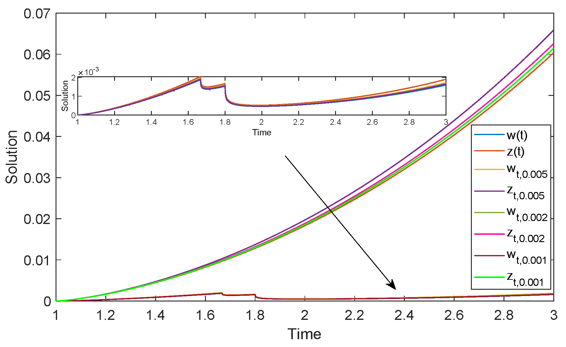
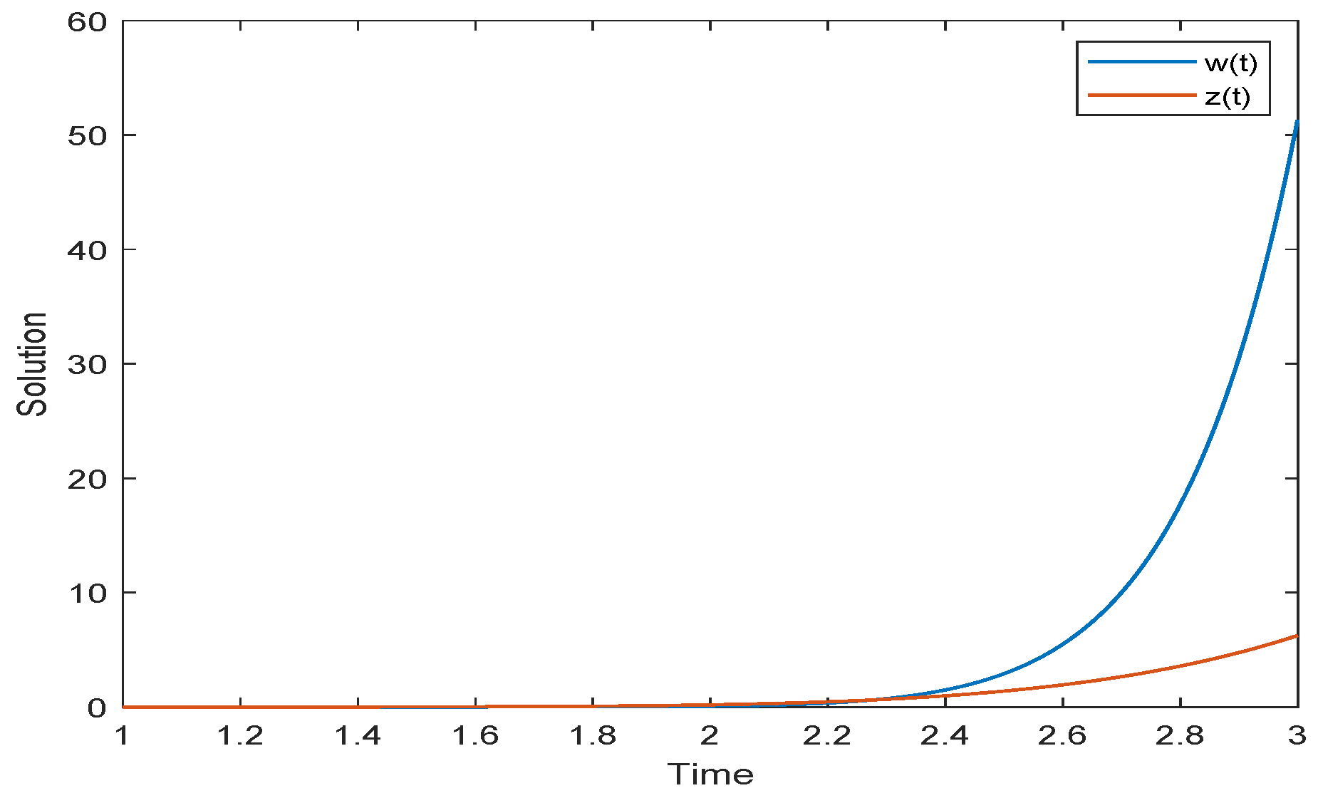
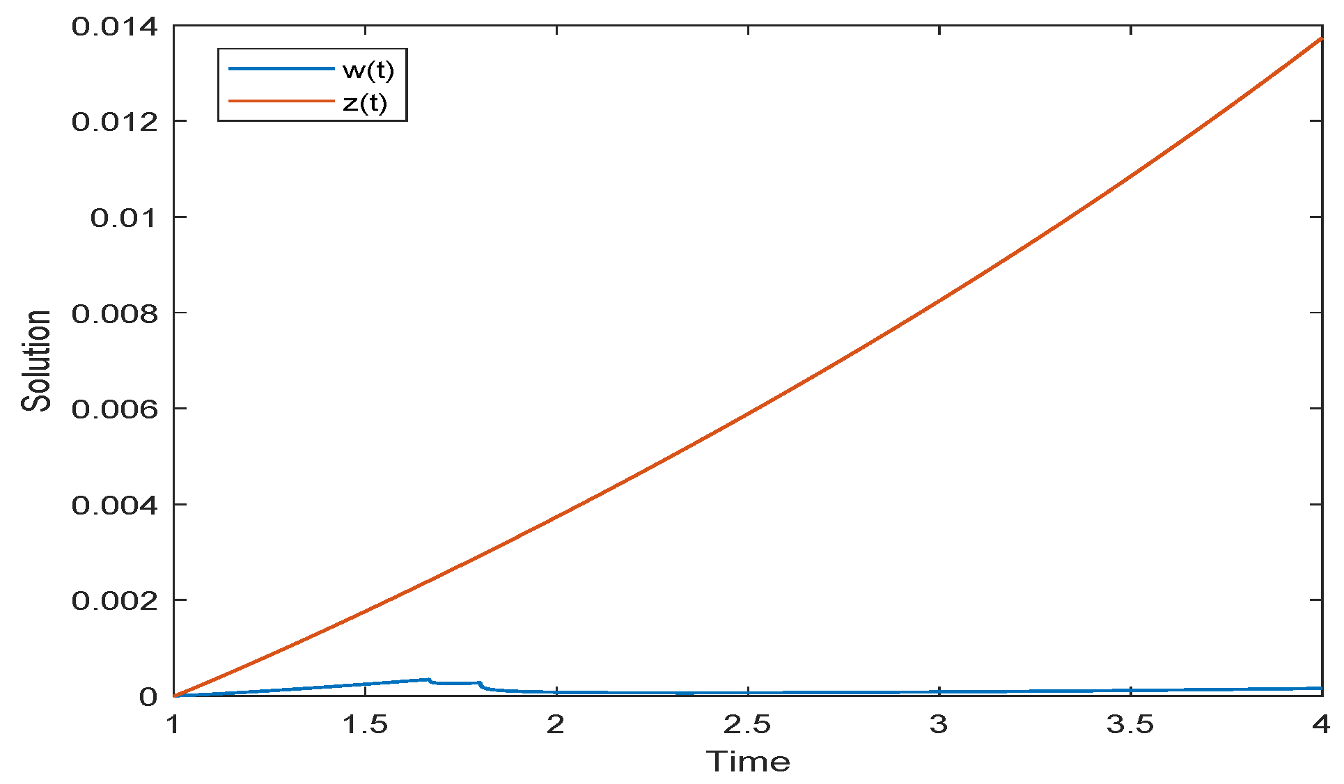
5. Examples and Simulations

Example 1.

Consider a nonlinear $(k,\psi )$-Hilfer fractional differential coupled Laplacian system as follows:

$$\begin{array}{c}\hfill \left\{\begin{array}{c}{}^{2,H}\mathcal{D}_{1^{+}}^{\frac{2}{3},\frac{1}{2},\psi }\left[{\Phi }_{\frac{3}{2}}{(}^{2,H}{\mathcal{D}}_{1^{+}}^{\frac{3}{2},\frac{1}{2},\psi }w\left(t\right))\right]=F_1(t,w\left(t\right),z\left(t\right)),1\le t\le 3,\hfill \\ {}^{2,H}\mathcal{D}_{1^{+}}^{\frac{1}{3},\frac{1}{3},\psi }\left[{\Phi }_2{(}^{2,H}{\mathcal{D}}_{1^{+}}^{\frac{4}{3},\frac{1}{3},\psi }z\left(t\right))\right]=F_2(t,w\left(t\right),z\left(t\right)),1\le t\le 3,\hfill \\ w\left(1\right)=0,{}^{2,H}\mathcal{D}_{1^{+}}^{\frac{3}{2},\frac{1}{2},\psi }w\left(1\right)=0,\hfill \\ w\left(3\right)=\frac{1}{30}{}^{2,H}\mathcal{D}_{1^{+}}^{\frac{1}{2},\frac{1}{2},\psi }z\left(\frac{5}{3}\right)+\frac{1}{20}{}^{2,H}\mathcal{D}_{1^{+}}^{\frac{1}{3},\frac{1}{4},\psi }z\left(\frac{9}{5}\right)+\frac{1}{20}{}^2\mathcal{J}_{1^{+}}^{\frac{1}{3},\psi }z\left(\frac{5}{2}\right)+\frac{1}{30}{}^2\mathcal{J}_{1^{+}}^{\frac{1}{2},\psi }z\left(2\right),\hfill \\ z\left(1\right)=0,{}^{2,H}\mathcal{D}_{1^{+}}^{\frac{4}{3},\frac{1}{3},\psi }z\left(1\right)=0,\hfill \\ z\left(3\right)=\frac{1}{20}{}^{2,H}\mathcal{D}_{1^{+}}^{\frac{1}{3},\frac{1}{3},\psi }w\left(\frac{4}{3}\right)+\frac{1}{30}{}^{2,H}\mathcal{D}_{1^{+}}^{\frac{1}{2},\frac{1}{5},\psi }w\left(\frac{3}{2}\right)+\frac{1}{30}{}^2\mathcal{J}_{1^{+}}^{1,\psi }w\left(2\right)+\frac{1}{20}{}^2\mathcal{J}_{1^{+}}^{\frac{1}{2},\psi }w\left(\frac{5}{2}\right),\hfill \end{array}\right.\end{array}$$

(79)

where $F_1(t,w\left(t\right),z\left(t\right))=\frac{1}{20}{(t^2-1)}^{-\frac{1}{3}}+\frac{t^2-1}{400}|cos\left(w\left(t\right)\right)|+\frac{t^2-1}{640}|sin\left(z\left(t\right)\right)|$ and $F_2(t,$$w\left(t\right),$$z\left(t\right))$$=\frac{1}{20}{(t^2-1)}^{-\frac{1}{6}}+\frac{t^2-1}{400}(sin\left(w\left(t\right)\right)+1)+\frac{t^2-1}{800}|cos\left(z\left(t\right)\right)|$.

Based on the data given above, by calculation, for any $t\in [1,3]$, we obtain

$$|F_1(t,w\left(t\right),z\left(t\right))-F_1(t,w^{\ast }\left(t\right),z^{\ast }\left(t\right))|\le \frac{t^2-1}{400}|w\left(t\right)-w^{\ast }\left(t\right)|+\frac{t^2-1}{640}|z\left(t\right)-z^{\ast }\left(t\right)|,$$

$$|F_2(t,w\left(t\right),z\left(t\right))-F_2(t,w^{\ast }\left(t\right),z^{\ast }\left(t\right))|\le \frac{t^2-1}{400}|w\left(t\right)-w^{\ast }\left(t\right)|+\frac{t^2-1}{800}|z\left(t\right)-z^{\ast }\left(t\right)|.$$

Obviously, $L_{11}\left(t\right)=L_{21}\left(t\right)=\frac{t^2-1}{400}$, $L_{12}\left(t\right)=\frac{t^2-1}{640}$, $L_{22}\left(t\right)=\frac{t^2-1}{800}$, ${\parallel L_{11}\left(t\right)\parallel }_{[1,3]}$ = ${\parallel L_{21}\left(t\right)\parallel }_{[1,3]}$ = $\frac{1}{50}$, ${\parallel L_{12}\left(t\right)\parallel }_{[1,3]}=\frac{1}{80}$, ${\parallel L_{22}\left(t\right)\parallel }_{[1,3]}=\frac{1}{100}$, $q_1=3$, $q_2=2$. Furthermore, we choose ${\delta }_1=\frac{4}{3}$ and ${\delta }_2=\frac{5}{3}$, so, for $\forall (t,w,z)\in I\times {\mathbb{R}}^2$, $F_1(t,w\left(t\right),z\left(t\right))\le {(t^2-1)}^{-\frac{1}{3}}$ and $F_2(t,w\left(t\right),z\left(t\right))\le {(t^2-1)}^{-\frac{1}{6}}$. At the same time, we have ${\gamma }_{2k}=2.75$, ${\gamma }_{3k}\approx 2.2222$, $A_1\approx 1.892$, $A_2\approx 1.2319$, $B_1\approx 0.1946$, $B_2\approx 0.23$, $\Delta =A_1{A}_2-B_1{B}_2\approx 2.2859>0$, ${\Xi }_1\approx 6.9797$, ${\Xi }_2\approx 6.2983$, ${\overline{N}}_1=1.0748$, ${\overline{N}}_2=1.0056$, and

$${\mathcal{M}}_1=\underset{j=1,2}{max}\left\{\frac{(q_j-1){\overline{N}}_j^{q_j-2}}{{\Gamma }_k({\eta }_j+k)}{(\psi \left(d\right)-\psi \left(c\right))}^{\frac{{\eta }_j}{k}}({\parallel L_{j1}\parallel }_{[c,d]}+{\parallel L_{j2}\parallel }_{[c,d]})\right\}\approx 0.1242,$$

$${\varrho }_1={\mathcal{M}}_{1}max\left\{{\Xi }_1,{\Xi }_2\right\}\approx 0.8668<1.$$

Consequently, all the conditions of Theorems 1 and 7 are satisfied. According to Theorems 1 and 7, one knows that system (79) has a unique solution on $[1,3]$, which is GUH-stable.

Example 2.

Consider the following nonlinear $(k,\psi )$-Hilfer fractional differential coupled Laplacian system:

$$\begin{array}{c}\hfill \left\{\begin{array}{c}{}^{6,H}\mathcal{D}_{1^{+}}^{\frac{2}{3},\frac{1}{2},\psi }\left[{\Phi }_{\frac{5}{2}}{(}^{6,H}{\mathcal{D}}_{1^{+}}^{\frac{5}{3},\frac{1}{2},\psi }w\left(t\right))\right]=F_1(t,w\left(t\right),z\left(t\right)),1\le t\le 3,\hfill \\ {}^{6,H}\mathcal{D}_{1^{+}}^{\frac{1}{3},\frac{1}{3},\psi }\left[{\Phi }_{\frac{7}{3}}{(}^{6,H}{\mathcal{D}}_{1^{+}}^{\frac{7}{4},\frac{1}{3},\psi }z\left(t\right))\right]=F_1(t,w\left(t\right),z\left(t\right)),1\le t\le 3,\hfill \\ w\left(1\right)=0,{}^{6,H}\mathcal{D}_{1^{+}}^{\frac{5}{3},\frac{1}{2},\psi }w\left(1\right)=0,\hfill \\ w\left(3\right)=\frac{1}{30}{}^{6,H}\mathcal{D}_{1^{+}}^{\frac{1}{2},\frac{1}{2},\psi }z\left(\frac{5}{3}\right)+\frac{1}{20}{}^{6,H}\mathcal{D}_{1^{+}}^{\frac{1}{3},\frac{1}{4},\psi }z\left(\frac{9}{5}\right)+\frac{1}{20}{}^6\mathcal{J}_{1^{+}}^{\frac{1}{3},\psi }z\left(\frac{5}{2}\right)+\frac{1}{30}{}^6\mathcal{J}_{1^{+}}^{\frac{1}{2},\psi }z\left(2\right),\hfill \\ z\left(1\right)=0,{}^{6,H}\mathcal{D}_{1^{+}}^{\frac{7}{4},\frac{1}{3},\psi }z\left(1\right)=0,\hfill \\ z\left(3\right)=\frac{1}{20}{}^{6,H}\mathcal{D}_{1^{+}}^{\frac{1}{3},\frac{1}{3},\psi }w\left(\frac{4}{3}\right)+\frac{1}{30}{}^{6,H}\mathcal{D}_{1^{+}}^{\frac{1}{2},\frac{1}{5},\psi }w\left(\frac{3}{2}\right)+\frac{1}{30}{}^6\mathcal{J}_{1^{+}}^{1,\psi }w\left(2\right)+\frac{1}{20}{}^6\mathcal{J}_{1^{+}}^{\frac{1}{2},\psi }w\left(\frac{5}{2}\right),\hfill \end{array}\right.\end{array}$$

(80)

where $F_1(t,w\left(t\right),z\left(t\right))={(t^2-1)}^{\frac{8}{3}}+\frac{2+cos\left(2t\right)}{20}\left[\right|arctan\left(w\left(t\right)\right)|+|\mathrm{arccot}\left(z\left(t\right)\right)\left|\right]$ and $F_2(t,$$w\left(t\right),$$z\left(t\right))$ = ${(t^2-1)}^{\frac{5}{2}}+\frac{2+sin\left(2t\right)}{20}\left[\right|\mathrm{arccot}\left(w\left(t\right)\right)|+|arctan\left(z\left(t\right)\right)\left|\right]$.

By a simple calculation, we obtain

$$|F_1(t,w\left(t\right),z\left(t\right))-F_1(t,w^{\ast }\left(t\right),z^{\ast }\left(t\right))|\le \frac{2+cos\left(2t\right)}{20}\left[|w\left(t\right)-w^{\ast }\left(t\right)|+|z\left(t\right)-z^{\ast }\left(t\right)|\right],$$

$$|F_2(t,w\left(t\right),z\left(t\right))-F_2(t,w^{\ast }\left(t\right),z^{\ast }\left(t\right))|\le \frac{2+sin\left(2t\right)}{20}\left[|w\left(t\right)-w^{\ast }\left(t\right)|+|z\left(t\right)-z^{\ast }\left(t\right)|\right].$$

Clearly, $L_{11}\left(t\right)=L_{12}\left(t\right)=\frac{2+cos\left(2t\right)}{20}$, $L_{21}\left(t\right)=L_{22}\left(t\right)=\frac{2+sin\left(2t\right)}{20}$, ${\parallel L_{11}\left(t\right)\parallel }_{[1,3]}$ = ${\parallel L_{12}\left(t\right)\parallel }_{[1,3]}$ = ${\parallel L_{21}\left(t\right)\parallel }_{[1,3]}$ = ${\parallel L_{22}\left(t\right)\parallel }_{[1,3]}$ = $\frac{3}{20}$, $q_1=1.6667$, $q_2=1.75$. Furthermore, we choose ${\zeta }_1=\frac{22}{3}$ and ${\zeta }_2=7$, so $\forall (t,w,z)\in I\times {\mathbb{R}}^2$, $F_1(t,w\left(t\right),z\left(t\right))\ge {(t^2-1)}^{\frac{8}{3}}$, and $F_2(t,w\left(t\right),z\left(t\right))\ge {(t^2-1)}^{\frac{5}{2}}$. Meanwhile, we have ${\gamma }_{2k}\approx 6.8333$, ${\gamma }_{3k}\approx 5.1667$, $A_1\approx 1.111$, $A_2\approx 0.8718$, $B_1\approx 0.1704$, $B_2\approx 0.1587$, $\Delta =A_1{A}_2-B_1{B}_2\approx 0.9415>0$, ${\Xi }_1\approx 2.8691$, ${\Xi }_2\approx 2.8011$, $g_1{\Xi }_1-1\approx -0.0616<0$, $g_2{\Xi }_2-1\approx -0.1205<0$, and

$$\begin{array}{cc}\hfill {\mathcal{M}}_2=& \underset{j=1,2}{\max }\{\frac{(q_j-1)}{{\Gamma }_k({\eta }_j+k)}{\left(\frac{{\Gamma }_k\left({\zeta }_j\right)}{{\Gamma }_k({\zeta }_j+{\eta }_j)}\right)}^{q_j-2}{(\psi \left(d\right)-\psi \left(c\right))}^{((\frac{{\zeta }_j+{\eta }_j}{k}-1)(q_j-2)+\frac{{\eta }_j}{k})}\hfill \\ & \times ({\parallel L_{j1}\parallel }_{[c,d]}+{\parallel L_{j2}\parallel }_{[c,d]})\}\approx 0.2142,\hfill \end{array}$$

$${\varrho }_2={\mathcal{M}}_{2}max\left\{{\Xi }_1,{\Xi }_2\right\}\approx 0.6146<1.$$

Thus, all the conditions of Theorem 2 are also satisfied. According to Theorem 2, we claim that system (80) still has a unique solution on $[1,3]$.

Example 3.

Consider nonlinear $(k,\psi )$-Hilfer fractional differential coupled Laplacian systems of the form

$$\begin{array}{c}\hfill \left\{\begin{array}{c}{}^{2,H}\mathcal{D}_{1^{+}}^{\frac{2}{3},\frac{1}{2},\psi }\left[{\Phi }_{\frac{3}{2}}{(}^{2,H}{\mathcal{D}}_{1^{+}}^{\frac{3}{2},\frac{1}{2},\psi }w\left(t\right))\right]=F_1(t,w\left(t\right),z\left(t\right)),1\le t\le 4,\hfill \\ {}^{2,H}\mathcal{D}_{1^{+}}^{\frac{1}{3},\frac{1}{3},\psi }\left[{\Phi }_2{(}^{2,H}{\mathcal{D}}_{1^{+}}^{\frac{4}{3},\frac{1}{3},\psi }z\left(t\right))\right]=F_2(t,w\left(t\right),z\left(t\right)),1\le t\le 4,\hfill \end{array}\right.\end{array}$$

(81)

subject to the following boundary value conditions

$$\begin{array}{c}\hfill \left\{\begin{array}{c}w\left(1\right)=0,{}^{2,H}\mathcal{D}_{1^{+}}^{\frac{3}{2},\frac{1}{2},\psi }w\left(1\right)=0,\hfill \\ w\left(3\right)=\frac{1}{30}{}^{2,H}\mathcal{D}_{1^{+}}^{\frac{1}{2},\frac{1}{2},\psi }z\left(\frac{5}{3}\right)+\frac{1}{20}{}^{2,H}\mathcal{D}_{1^{+}}^{\frac{1}{3},\frac{1}{4},\psi }z\left(\frac{9}{5}\right)+\frac{1}{20}{}^2\mathcal{J}_{1^{+}}^{\frac{1}{3},\psi }z\left(\frac{5}{2}\right)+\frac{1}{30}{}^2\mathcal{J}_{1^{+}}^{\frac{1}{2},\psi }z\left(2\right),\hfill \\ z\left(1\right)=0,{}^{2,H}\mathcal{D}_{1^{+}}^{\frac{4}{3},\frac{1}{3},\psi }z\left(1\right)=0,\hfill \\ z\left(3\right)=\frac{1}{20}{}^{2,H}\mathcal{D}_{1^{+}}^{\frac{1}{3},\frac{1}{3},\psi }w\left(\frac{4}{3}\right)+\frac{1}{30}{}^{2,H}\mathcal{D}_{1^{+}}^{\frac{1}{2},\frac{1}{5},\psi }w\left(\frac{3}{2}\right)+\frac{1}{30}{}^2\mathcal{J}_{1^{+}}^{1,\psi }w\left(2\right)+\frac{1}{20}{}^2\mathcal{J}_{1^{+}}^{\frac{1}{2},\psi }w\left(\frac{5}{2}\right),\hfill \end{array}\right.\end{array}$$

where $F_1(t,w\left(t\right),z\left(t\right))=\frac{1}{20}{(t^2-1)}^{-\frac{1}{3}}+\frac{t^2-1}{900}|cos\left(w\left(t\right)\right)|+\frac{t^2-1}{1500}|sin\left(z\left(t\right)\right)|$ and $F_2(t,$$w\left(t\right),$$z\left(t\right))$ = $\frac{1}{20}{(t^2-1)}^{-\frac{1}{6}}+\frac{t^2-1}{900}(\sin \left(w\left(t\right)\right)+1)+\frac{t^2-1}{3000}\left|\cos \left(z\left(t\right)\right)\right|$.

From the given data, by a simple calculation, for any $t\in [1,4]$, we obtain

$$|F_1(t,w\left(t\right),z\left(t\right))-F_1(t,w^{\ast }\left(t\right),z^{\ast }\left(t\right))|\le \frac{t^2-1}{900}|w\left(t\right)-w^{\ast }\left(t\right)|+\frac{t^2-1}{1500}|z\left(t\right)-z^{\ast }\left(t\right)|,$$

$$|F_2(t,w\left(t\right),z\left(t\right))-F_2(t,w^{\ast }\left(t\right),z^{\ast }\left(t\right))|\le \frac{t^2-1}{900}|w\left(t\right)-w^{\ast }\left(t\right)|+\frac{t^2-1}{3000}|z\left(t\right)-z^{\ast }\left(t\right)|.$$

Clearly, $L_{11}\left(t\right)=L_{21}\left(t\right)=\frac{t^2-1}{900}$, $L_{12}\left(t\right)=\frac{t^2-1}{1500}$, $L_{22}\left(t\right)=\frac{t^2-1}{3000}$, ${\parallel L_{11}\left(t\right)\parallel }_{[1,4]}$ = ${\parallel L_{21}\left(t\right)\parallel }_{[1,4]}$ = $\frac{1}{60}$, ${\parallel L_{12}\left(t\right)\parallel }_{[1,4]}=\frac{1}{100}$, ${\parallel L_{22}\left(t\right)\parallel }_{[1,4]}=\frac{1}{200}$, $q_1=3$, and $q_2=2$. We choose ${\delta }_1=\frac{4}{3}$ and ${\delta }_2=\frac{5}{3}$, so, for $\forall (t,w,z)\in [1,4]\times {\mathbb{R}}^2$, $F_1(t,w\left(t\right),z\left(t\right))\le {(t^2-1)}^{-\frac{1}{3}}$ and $F_2(t,w\left(t\right),z\left(t\right))\le {(t^2-1)}^{-\frac{1}{6}}$. At the same time, we obtain ${\gamma }_{2k}\approx 2.2222$, ${\gamma }_{3k}\approx 2.75$, $A_1\approx 1.321$, $A_2\approx 2.3949$, $B_1\approx 0.2336$, $B_2\approx 0.2105$, $\Delta =A_1{A}_2-B_1{B}_2\approx 3.1144>0$, ${\Xi }_1\approx 9.349$, ${\Xi }_2\approx 10.9155$, ${\overline{N}}_1\approx 1.0748$, ${\overline{N}}_2\approx 1.0056$, and

$${\mathcal{M}}_1=\underset{j=1,2}{max}\left\{\frac{(q_j-1){\overline{N}}_j^{q_j-2}}{{\Gamma }_k({\eta }_j+k)}{(\psi \left(d\right)-\psi \left(c\right))}^{\frac{{\eta }_j}{k}}({\parallel L_{j1}\parallel }_{[c,d]}+{\parallel L_{j2}\parallel }_{[c,d]})\right\}\approx 0.1256,$$

$${\varrho }_1={\mathcal{M}}_{1}max\left\{{\Xi }_1,{\Xi }_2\right\}\approx 1.3715>1,$$

$${\varrho }_3={\mathcal{M}}_1\underset{j=1,2}{max}\left\{{\Xi }_j-\frac{{(\psi \left(d\right)-\psi \left(c\right))}^{\frac{{\alpha }_j}{k}}}{{\Gamma }_k({\alpha }_j+k)}\right\}\approx 0.7519<1.$$

Thus, all the conditions of Theorem 4 are satisfied. According to Theorem 4, we claim that system (81) has a solution on $[1,4]$. It is worth noting that the condition $\left({\mathrm{H}}_4\right)$ of Theorem 1 is not satisfied, so Theorem 1 cannot be used to analyze the existence of system (81).

To solve the numerical solution of Examples 1–3, we first make $u\left(t\right)={}^k\mathcal{J}_{c^{+}}^{{\eta }_1,\psi }{F}_1(t,w\left(t\right),z\left(t\right))$ and $v\left(t\right)={}^k\mathcal{J}_{c^{+}}^{{\eta }_2,\psi }{F}_2(t,w\left(t\right),z\left(t\right))$; then, it follows from the proof of Lemma 10 that system (4) transforms into the following nonlinear integral coupled system (82)

$$\begin{array}{c}\hfill \left\{\begin{array}{c}w\left(t\right)={}^k\mathcal{J}_{c^{+}}^{{\alpha }_1,\psi }\left[{\Phi }_{q_1}\left(u\left(t\right)\right)\right]+{\mathcal{V}}_1(t,u\left(t\right),v\left(t\right)),\hfill \\ z\left(t\right)={}^k\mathcal{J}_{c^{+}}^{{\alpha }_2,\psi }\left[{\Phi }_{q_2}\left(v\left(t\right)\right)\right]+{\mathcal{V}}_2(t,u\left(t\right),v\left(t\right)),\hfill \\ u\left(t\right)={}^k\mathcal{J}_{c^{+}}^{{\eta }_1,\psi }{F}_1(t,w\left(t\right),z\left(t\right)),\hfill \\ v\left(t\right)={}^k\mathcal{J}_{c^{+}}^{{\eta }_2,\psi }{F}_2(t,w\left(t\right),z\left(t\right)),\hfill \end{array}\right.\end{array}$$

(82)

where

$$\begin{array}{cc}\hfill {\mathcal{V}}_1& (t,u\left(t\right),v\left(t\right))=\frac{1}{\Delta {\Gamma }_k\left({\gamma }_{2k}\right)}\{A_2\sum _{i=1}^m{\lambda }_{1i}{}^k\mathcal{J}_{c^{+}}^{{\alpha }_2-l_i,\psi }\left[{\Phi }_{q_2}\left(v\left(t\right)\right)\right]{|}_{t={\xi }_i}\hfill \\ \hfill & -A_2{}^k\mathcal{J}_{c^{+}}^{{\alpha }_1,\psi }\left[{\Phi }_{q_1}\left(u\left(t\right)\right)\right]{|}_{t=d}+A_2\sum _{i=1}^m{\lambda }_{2i}{}^k\mathcal{J}_{c^{+}}^{{\alpha }_2+{\sigma }_i,\psi }\left[{\Phi }_{q_2}\left(v\left(t\right)\right)\right]{|}_{t={\xi }_i^{\ast }}\hfill \end{array}$$

$$\begin{array}{cc}\hfill & -B_1{}^k\mathcal{J}_{c^{+}}^{{\alpha }_2,\psi }\left[{\Phi }_{q_2}\left(v\left(t\right)\right)\right]{|}_{t=d}+B_1\sum _{i=1}^m{\mu }_{1i}{}^k\mathcal{J}_{c^{+}}^{{\alpha }_1-l_i^{\ast },\psi }\left[{\Phi }_{q_1}\left(u\left(t\right)\right)\right]{|}_{t={\theta }_i}\hfill \\ \hfill & +B_1\sum _{i=1}^m{\mu }_{2i}{}^k\mathcal{J}_{c^{+}}^{{\alpha }_1+{\sigma }_i^{\ast },\psi }\left[{\Phi }_{q_1}\left(u\left(t\right)\right)\right]{|}_{t={\theta }_i^{\ast }}\}{(\psi \left(t\right)-\psi \left(c\right))}^{\frac{{\gamma }_{2k}}{k}-1},\hfill \end{array}$$

and

$$\begin{array}{cc}\hfill {\mathcal{V}}_2& (t,u\left(t\right),v\left(t\right))=\frac{1}{\Delta {\Gamma }_k\left({\gamma }_{3k}\right)}\{A_1\sum _{i=1}^m{\mu }_{1i}{}^k\mathcal{J}_{c^{+}}^{{\alpha }_1-l_i^{\ast },\psi }\left[{\Phi }_{q_1}\left(u\left(t\right)\right)\right]{|}_{t={\theta }_i}\hfill \\ \hfill & -A_1{}^k\mathcal{J}_{c^{+}}^{{\alpha }_2,\psi }\left[{\Phi }_{q_2}\left(v\left(t\right)\right)\right]{|}_{t=d}+A_1\sum _{i=1}^m{\mu }_{2i}{}^k\mathcal{J}_{c^{+}}^{{\alpha }_1+{\sigma }_i^{\ast },\psi }\left[{\Phi }_{q_1}\left(u\left(t\right)\right)\right]{|}_{t={\theta }_i^{\ast }}\hfill \\ \hfill & -B_2{}^k\mathcal{J}_{c^{+}}^{{\alpha }_1,\psi }\left[{\Phi }_{q_1}\left(u\left(t\right)\right)\right]{|}_{t=d}+B_2\sum _{i=1}^m{\lambda }_{1i}{}^k\mathcal{J}_{c^{+}}^{{\alpha }_2-l_i,\psi }\left[{\Phi }_{q_2}\left(v\left(t\right)\right)\right]{|}_{t={\xi }_i}\hfill \\ \hfill & +B_2\sum _{i=1}^m{\lambda }_{2i}{}^k\mathcal{J}_{c^{+}}^{{\alpha }_2+{\sigma }_i,\psi }\left[{\Phi }_{q_2}\left(v\left(t\right)\right)\right]{|}_{t={\xi }_i^{\ast }}\}{(\psi \left(t\right)-\psi \left(c\right))}^{\frac{{\gamma }_{3k}}{k}-1}.\hfill \end{array}$$

Secondly, after taking the derivative on both sides of Equation (82), the nonlinear integral coupled system (82) becomes the first-order differential Equation (83). Next, we can use the appropriate ODE toolbox in MATLAB to complete the numerical solution and simulation of Examples 1–3.

$$\begin{array}{c}\hfill \left\{\begin{array}{c}\frac{dw\left(t\right)}{dt}=\frac{1}{k}\frac{d\psi }{dt}\{{}^k\mathcal{J}_{c^{+}}^{{\alpha }_1-k,\psi }\left[{\Phi }_{q_1}\left(u\left(t\right)\right)\right]+{\mathcal{N}}_1(t,u\left(t\right),v\left(t\right))\},\hfill \\ \frac{dz\left(t\right)}{dt}=\frac{1}{k}\frac{d\psi }{dt}\{{}^k\mathcal{J}_{c^{+}}^{{\alpha }_2-k,\psi }\left[{\Phi }_{q_2}\left(v\left(t\right)\right)\right]+{\mathcal{N}}_2(t,u\left(t\right),v\left(t\right))\},\hfill \\ \frac{du\left(t\right)}{dt}=\frac{1}{k}\frac{d\psi }{dt}{}^k\mathcal{J}_{c^{+}}^{{\eta }_1-k,\psi }{F}_1(t,w\left(t\right),z\left(t\right)),\hfill \\ \frac{dv\left(t\right)}{dt}=\frac{1}{k}\frac{d\psi }{dt}{}^k\mathcal{J}_{c^{+}}^{{\eta }_2-k,\psi }{F}_2(t,w\left(t\right),z\left(t\right)),\hfill \end{array}\right.\end{array}$$

(83)

where

$$\begin{array}{cc}\hfill {\mathcal{N}}_1& (t,u\left(t\right),v\left(t\right))=\frac{{\gamma }_{2k}-k}{\Delta {\Gamma }_k\left({\gamma }_{2k}\right)}(A_2\sum _{i=1}^m{\lambda }_{1i}{}^k\mathcal{J}_{c^{+}}^{{\alpha }_2-l_i,\psi }\left[{\Phi }_{q_2}\left(v\left(t\right)\right)\right]{|}_{t={\xi }_i}\hfill \\ \hfill & -A_2{}^k\mathcal{J}_{c^{+}}^{{\alpha }_1,\psi }\left[{\Phi }_{q_1}\left(u\left(t\right)\right)\right]{|}_{t=d}+A_2\sum _{i=1}^m{\lambda }_{2i}{}^k\mathcal{J}_{c^{+}}^{{\alpha }_2+{\sigma }_i,\psi }\left[{\Phi }_{q_2}\left(v\left(t\right)\right)\right]{|}_{t={\xi }_i^{\ast }}\hfill \\ \hfill & -B_1{}^k\mathcal{J}_{c^{+}}^{{\alpha }_2,\psi }\left[{\Phi }_{q_2}\left(v\left(t\right)\right)\right]{|}_{t=d}+B_1\sum _{i=1}^m{\mu }_{1i}{}^k\mathcal{J}_{c^{+}}^{{\alpha }_1-l_i^{\ast },\psi }\left[{\Phi }_{q_1}\left(u\left(t\right)\right)\right]{|}_{t={\theta }_i}\hfill \\ \hfill & +B_1\sum _{i=1}^m{\mu }_{2i}{}^k\mathcal{J}_{c^{+}}^{{\alpha }_1+{\sigma }_i^{\ast },\psi }\left[{\Phi }_{q_1}\left(u\left(t\right)\right)\right]{|}_{t={\theta }_i^{\ast }})\times {(\psi \left(t\right)-\psi \left(c\right))}^{\frac{{\gamma }_{2k}}{k}-2},\hfill \end{array}$$

and

$$\begin{array}{cc}\hfill {\mathcal{N}}_2& (t,u\left(t\right),v\left(t\right))=\frac{{\gamma }_{3k}-k}{\Delta {\Gamma }_k\left({\gamma }_{3k}\right)}(A_1\sum _{i=1}^m{\mu }_{1i}{}^k\mathcal{J}_{c^{+}}^{{\alpha }_1-l_i^{\ast },\psi }\left[{\Phi }_{q_1}\left(u\left(t\right)\right)\right]{|}_{t={\theta }_i}\hfill \\ \hfill & -A_1{}^k\mathcal{J}_{c^{+}}^{{\alpha }_2,\psi }\left[{\Phi }_{q_2}\left(v\left(t\right)\right)\right]{|}_{t=d}+A_1\sum _{i=1}^m{\mu }_{2i}{}^k\mathcal{J}_{c^{+}}^{{\alpha }_1+{\sigma }_i^{\ast },\psi }\left[{\Phi }_{q_1}\left(u\left(t\right)\right)\right]{|}_{t={\theta }_i^{\ast }}\hfill \\ \hfill & -B_2{}^k\mathcal{J}_{c^{+}}^{{\alpha }_1,\psi }\left[{\Phi }_{q_1}\left(u\left(t\right)\right)\right]{|}_{t=d}+B_2\sum _{i=1}^m{\lambda }_{1i}{}^k\mathcal{J}_{c^{+}}^{{\alpha }_2-l_i,\psi }\left[{\Phi }_{q_2}\left(v\left(t\right)\right)\right]{|}_{t={\xi }_i}\hfill \\ \hfill & +B_2\sum _{i=1}^m{\lambda }_{2i}{}^k\mathcal{J}_{c^{+}}^{{\alpha }_2+{\sigma }_i,\psi }\left[{\Phi }_{q_2}\left(v\left(t\right)\right)\right]{|}_{t={\xi }_i^{\ast }})\times {(\psi \left(t\right)-\psi \left(c\right))}^{\frac{{\gamma }_{3k}}{k}-2}.\hfill \end{array}$$

Based on the above concise algorithm, we take the initial value $\left(w\right(c),z(c\left)\right)=(0,0)$ and apply the ODE45 toolbox in MATLAB R2018b to complete the numerical simulations of systems (79)–(81) and the GUH stability of system (79) shown in Figure 1, Figure 2, Figure 3 and Figure 4 outlined below. Figure 1 and Figure 2 simulate the solution’s evolution and GUH stability of system (79), respectively. Figure 3 simulates the solution’s evolution of system (80). Figure 4 simulates the solution’s evolution of system (81).

6. Conclusions

In this article, we mainly studied the multi-point symmetric integral boundary value problem for nonlinear $(k,\psi )$-Hilfer fractional differential coupled Laplacian Equation (4). Using Banach’s contraction mapping principle and the Krasnosel’skii fixed-point theorem, we obtain some meaningful and easily verifiable sufficient conditions on the existence and uniqueness of solutions to this problem. Furthermore, we also prove the GUH stability of this system using the calculus inequality technique. Finally, three interesting examples and numerical simulations are given to further verify the correctness and effectiveness of the conclusions. It is important that our results are of a more general nature and yield some new results in special cases. For example, the conclusion of the $(k,\psi )$-RL fractional differential coupled Laplacian equations are a result of fixing ${\beta }_i=0$, $i=1,2$ in the obtained results. On the other hand, by taking ${\beta }_i=1$, $i=1,2$ in the results of this paper, we obtain the ones for nonlinear $(k,\psi )$-Caputo fractional differential coupled Laplacian equations. Moreover, our results degenerate to the ones for a Laplacian system involving k-Hilfer–Hadamard fractional derivative operators and k-Hilfer–Katugampola fractional derivative operators by letting $\psi \left(t\right)=logt$ and $\psi \left(t\right)=t^{\rho }$, respectively. Furthermore, inspired by recent works [7,8,28,31,32], we can apply the fractional differential equation theory and fixed-point theorems to study $(k,\psi )$-Hilfer pseudo-fractional differential Laplacian equations and $(k,\psi )$-Hilfer fractional differential Laplacian equations with impulses and random effects in the future.

References

1. Dineshkumar, C.; Udhayakumar, R.; Vijayakumar, V.; Nisar, K. A discussion on the approximate controllability of Hilfer fractional neutral stochastic integro-differential systems. Chaos Solitons Fractals 2020, 142, 110472. [Google Scholar] [CrossRef]
2. Baleanu, D.; Jajarmi, A.; Mohammadi, H.; Rezapour, S. A new study on the mathematical modelling of human liver with Caputo-Fabrizio fractional derivative. Chaos Solitons Fractals 2020, 134, 109705. [Google Scholar] [CrossRef]
3. Lv, X.; Zhao, K.; Xie, H. Ulam-Hyers Stability and Simulation of a Delayed Fractional Differential Equation with Riemann-Stieltjes Integral Boundary Conditions and Fractional Impulses. Axioms 2024, 13, 682. [Google Scholar] [CrossRef]
4. Muthaiah, S.; Murugesan, M.; Awadalla, M.; Unyong, B.; Egami, R. Ulam-Hyers stability and existence results for a coupled sequential Hilfer-Hadamard-type integrodifferential system. AIMS Math. 2024, 9, 16203–16233. [Google Scholar] [CrossRef]
5. Tudorache, A.; Luca, R. Systems of Hilfer-Hadamard Fractional Differential Equations with Nonlocal Coupled Boundary Conditions. Fractal Fract. 2023, 7, 816. [Google Scholar] [CrossRef]
6. Zhao, K. Study on the stability and its simulation algorithm of a nonlinear impulsive ABC-fractional coupled system with a Laplacian operator via F-contractive mapping. Adv. Contin. Discret. Model 2024, 2024, 5. [Google Scholar] [CrossRef]
7. Díaz, R.; Pariguan, E. On hypergeometric functions and Pochhammer k-symbol. Divulg. Mat. 2007, 15, 179–192. [Google Scholar]
8. Mubeen, S.; Habibullah, G. k-fractional integrals and application. Int. J. Contemp. Math. Sci. 2012, 2, 89–94. [Google Scholar]
9. Dorrego, G. An alternative definition for the k-Riemann–Liouville fractional derivative. Appl. Math. Sci. 2015, 9, 481–491. [Google Scholar] [CrossRef]
10. Kilbas, A.; Srivastava, H.; Trujillo, J. Theory and Applications of the Fractional Differential Equations; Elsevier: Amsterdam, The Netherlands, 2006; Volume 204. [Google Scholar]
11. Sousa, J.; Oliveira, E. On the ψ-Hilfer fractional derivative. Commun. Nonlinear Sci. Numer. Simul. 2018, 60, 72–91. [Google Scholar] [CrossRef]
12. Kucche, K.; Mali, A. On the nonlinear (k, ψ)-Hilfer fractional differential equations. Chaos Solitons Fractals 2021, 152, 111335. [Google Scholar] [CrossRef]
13. Samadi, A.; Ntouyas, S.; Tariboon, J. Nonlocal Coupled System for (k, ψ)-Hilfer Fractional Differential Equations. Fractal Fract. 2022, 6, 234. [Google Scholar] [CrossRef]
14. Kharade, J.; Kucche, K. On the (k, ψ)-Hilfer nonlinear impulsive fractional differential equations. Math. Methods Appl. Sci. 2023, 46, 16282–16304. [Google Scholar] [CrossRef]
15. Kamsrisuk, N.; Ntouyas, S.; Ahmad, B.; Samadi, A.; Tariboon, J. Existence results for a coupled system of (k, ψ)-Hilfer fractional differential equations with nonlocal integro-multi-point boundary conditions. AIMS Math. 2023, 8, 4079–4097. [Google Scholar] [CrossRef]
16. Samadi, A.; Ntouyas, S.; Ahmad, B.; Samadi, A.; Tariboon, J. On a Coupled Differential System Involving (k, ψ)-Hilfer Derivative and (k, ψ)-Riemann-Liouville Integral Operators. Axioms 2023, 12, 229. [Google Scholar] [CrossRef]
17. Samadi, A.; Ntouyas, S.; Tariboon, J. Study on a Nonlocal Fractional Coupled System Involving (k, ψ)-Hilfer Derivatives and (k, ψ)-Riemann-Liouville Integral Operators. Fractal Fract. 2024, 8, 211. [Google Scholar] [CrossRef]
18. Leibenson, L. General problem of the movement of a compressible uid in a porous medium. Izv. Akad. Nauk Kirg. SSR Ser. Biol. Nauk 1983, 9, 7–10. [Google Scholar]
19. Zhao, K. Solvability, Approximation and Stability of Periodic Boundary Value Problem for a Nonlinear Hadamard Fractional Differential Equation with p-Laplacian. Axioms 2023, 12, 733. [Google Scholar] [CrossRef]
20. Khan, H.; Chen, W.; Sun, H. Analysis of positive solution and Hyers-Ulam stability for a class of singular fractional differential equations with p-Laplacian in Banach space. Math. Methods Appl. Sci. 2018, 41, 3430–3440. [Google Scholar] [CrossRef]
21. Lv, X.; Zhao, K.; Xie, H. Stability and Numerical Simulation of a Nonlinear Hadamard Fractional Coupling Laplacian System with Symmetric Periodic Boundary Conditions. Symmetry 2024, 16, 774. [Google Scholar] [CrossRef]
22. Li, S.; Zhang, Z.; Jiang, W. Multiple positive solutions for four-point boundary value problem of fractional delay differential equations with p-Laplacian operator. Appl. Numer. Math. 2021, 165, 348–356. [Google Scholar] [CrossRef]
23. Rao, S.; Ahmadini, A. Multiple positive solutions for system of mixed Hadamard fractional boundary value problems with (p1, p2)-Laplacian operator. AIMS Math. 2023, 8, 14767–14791. [Google Scholar] [CrossRef]
24. Zhao, K. Stability of a nonlinear Langevin system of ML-type fractional derivative affected by time-varying delays and differential feedback control. Fractal Fract. 2022, 6, 725. [Google Scholar] [CrossRef]
25. Abbas, S.; Benchohra, M.; Lagreg, J.; Alsaedi, A.; Zhou, Y. Existence and Ulam stability for fractional differential equations of Hilfer-Hadamard type. Adv. Differ. Equ. 2017, 2017, 180. [Google Scholar] [CrossRef]
26. Ho, V.; Ngo, V. Hyers-Ulam stability of fuzzy fractional Volterra integral equations with the kernel ψ-function via successive approximation method. Fuzzy Set. Syst. 2021, 419, 67–98. [Google Scholar]
27. Sousa, J.; Oliveira, E. On the Ulam-Hyers-Rassias stability for nonlinear fractional differential equations using the ψ-Hilfer operator. J. Fixed Point Theory Appl. 2018, 20, 96. [Google Scholar] [CrossRef]
28. Zhao, K.; Liu, J.; Lv, X. A unified approach to solvability and stability of multipoint BVPs for Langevin and Sturm–Liouville equations with CH–fractional derivatives and impulses via coincidence Theory. Fractal Fract. 2024, 8, 111. [Google Scholar] [CrossRef]
29. Murugesan, M.; Muthaiah, S.; Alzabut, J.; Gopal, T. Existence and H-U stability of a tripled system of sequential fractional differential equations with multipoint boundary conditions. Bound. Value Probl. 2023, 2023, 56. [Google Scholar] [CrossRef]
30. Ahmed, A.; Madeaha, A.; Bashir, A. Uniqueness of solutions for a ψ-Hilfer fractional integral boundary value problem with the p-Laplacian operator. Demonstr. Math. 2023, 56, 20220195. [Google Scholar]
31. Selvam, A.; Govindaraj, V.; Ahmad, H. Examining reachability criteria for fractional dynamical systems with mixed delays in control utilizing ψ-Hilfer pseudo-fractional derivative. Chaos Solitons Fractals 2024, 181, 114702. [Google Scholar] [CrossRef]
32. Abbas, S.; Benchohra, M.; Zhou, Y. Coupled Hilfer fractional differential systems with random effects. Adv. Differ. Equ. 2018, 2018, 369. [Google Scholar] [CrossRef]
Figure 1. Numerical simulation of solutions ( w ( t ) , z ( t ) ) for system (79).
Symmetry 17 00472 g001
Figure 2. Evolution of GUH stability with ϵ = 0.001, 0.002, 0.005 for system (79).
Symmetry 17 00472 g002
Figure 3. Numerical simulation of solutions ( w ( t ) , z ( t ) ) for system (80).
Symmetry 17 00472 g003
Figure 4. Numerical simulation of solutions ( w ( t ) , z ( t ) ) for system (81).
Symmetry 17 00472 g004
Disclaimer/Publisher’s Note: The statements, opinions and data contained in all publications are solely those of the individual author(s) and contributor(s) and not of MDPI and/or the editor(s). MDPI and/or the editor(s) disclaim responsibility for any injury to people or property resulting from any ideas, methods, instructions or products referred to in the content.