Abstract
Neural Radiance Fields (NeRF) have transformed 3D reconstruction by enabling high-fidelity scene generation from sparse views. However, existing neural SLAM systems face challenges such as limited scene understanding and heavy reliance on depth sensors. We propose UE-SLAM, a real-time monocular SLAM system integrating semantic segmentation, depth fusion, and robust tracking modules. By leveraging the inherent symmetry between semantic segmentation and depth estimation, UE-SLAM utilizes DINOv2 for instance segmentation and combines monocular depth estimation, radiance field-rendered depth, and an uncertainty framework to produce refined proxy depth. This approach enables high-quality semantic mapping and eliminates the need for depth sensors. Experiments on benchmark datasets demonstrate that UE-SLAM achieves robust semantic segmentation, detailed scene reconstruction, and accurate tracking, significantly outperforming existing monocular SLAM methods. The modular and symmetrical architecture of UE-SLAM ensures a balance between computational efficiency and reconstruction quality, aligning with the thematic focus of symmetry in engineering and computational systems.
1. Introduction
In recent years, with the rapid development of novel view synthesis techniques, the fields of computer vision and 3D reconstruction have made significant progress [1,2,3,4,5]. Among these advancements, Neural Radiance Fields (NeRF) [6] have emerged as a groundbreaking approach, garnering widespread attention from both academia and industry. NeRF enable the generation of high-fidelity 3D scenes from sparse input views, which is crucial for applications that require precise understanding and representation of the environment, such as virtual reality (VR), augmented reality (AR), robotics, and autonomous navigation. The ability to synthesize novel views from a small set of input images enables realistic scene rendering, enhancing immersive experiences and facilitating real-time interaction.
A noteworthy feature of NeRF-based systems, particularly in the context of SLAM, is their ability to maintain symmetrical properties in 3D reconstructions. This is important in ensuring that reconstructed environments preserve geometric consistency, contributing to more accurate navigation and map generation. The symmetry of a scene, whether in static or dynamic conditions, plays a crucial role in improving the precision of mapping algorithms and ensuring the coherence of the generated 3D models. This capability aligns with Symmetry’s focus on the theoretical and practical aspects of symmetrical properties in computational models and real-world applications.
One of the key advantages of NeRF is their real-time performance, making them particularly well-suited for dynamic environments that require rapid updates and interactions. This characteristic naturally facilitates the integration of NeRF with Simultaneous Localization and Mapping (SLAM) [7,8,9,10], an important technology that enables autonomous agents to navigate and comprehend their surroundings. The combination of NeRF and SLAM holds the potential to achieve real-time, high-precision, and highly detailed 3D mapping, significantly enhancing the capabilities of robotic systems and other autonomous platforms. Furthermore, the ability to update and refine 3D maps continuously as an agent moves through its environment is a key step toward fully autonomous systems capable of navigating unknown or changing landscapes with high fidelity, all while respecting the symmetry and structure of the physical world.
However, despite these potential advantages, current neural implicit SLAM systems still face several significant challenges. One primary issue is the difficulty in scene understanding. Existing SLAM systems often lack flexible scene comprehension due to the absence of a dedicated semantic module, which hinders effective object-level segmentation. Without semantic segmentation, these systems struggle to differentiate between objects and their surroundings, making it challenging to handle dynamic environments or specific object interactions. Furthermore, the lack of symmetry in scene reconstruction can lead to inconsistencies in object representation, which further complicates the system’s ability to accurately track and map dynamic elements. In this context, leveraging symmetry—whether through inherent geometric regularities or learned representations—could significantly improve object detection and segmentation accuracy, facilitating more robust SLAM performance.
Additionally, many of these systems rely heavily on depth sensors, which limits their adaptability and scalability. In environments where depth information is sparse or unavailable, performance tends to degrade significantly. The absence of symmetry in the representation of 3D objects exacerbates this issue, as objects without clear geometric patterns are harder to recognize and track. This dependence on depth sensors also introduces additional computational complexity and hardware requirements, further limiting the portability and efficiency of the systems, especially in resource-constrained scenarios. By incorporating symmetry into neural implicit models, one could reduce the reliance on detailed depth data and improve robustness across a wider range of environments.
To address these limitations, we introduce UE-SLAM, a real-time dense SLAM system designed for monocular RGB input. Our key contributions include leveraging DINOv2 [11] for instance segmentation, integrating monocular depth estimation from DepthAnythingV2 [12], radiance field-rendered depth, and an MLP-based uncertainty framework to produce refined proxy depth. We then combine this depth with tri-plane features to obtain a TSDF [13] representation, enhancing geometric and texture fidelity. Additionally, our tracking module employs proxy depth and photometric error minimization for robust per-pixel tracking, ensuring accurate motion estimation across frames. This integration enables real-time, highly accurate mapping and localization, even in complex, dynamic environments.
Our experimental results demonstrate that UE-SLAM effectively generates robust semantic segmentation results, high-quality scene texture and detail representation, and simultaneously constructs a semantic map. This addresses the critical limitations of current monocular neural implicit SLAM systems, which either depend on RGB-D inputs or lack semantic segmentation capabilities. Furthermore, our method is designed to operate without relying on external depth sensors, making it suitable for real-world applications where such sensors may be unavailable or impractical. The key contributions of our approach can be summarized as follows:
- We propose UE-SLAM, a real-time dense SLAM system designed for monocular RGB input. It comprises a semantic segmentation module, proxy depth fusion module, implicit reconstruction module, and frame-to-frame tracking module. Our system achieves robust semantic map reconstruction while preserving texture details, without relying on depth sensors.
- We introduce a novel proxy depth model, which integrates monocular depth estimation, radiance field-rendered depth, local semantic information, and an uncertainty framework to perform depth fusion. This approach produces a refined proxy depth, effectively mitigating the dependency on external depth sensors while maintaining high accuracy.
- Both the tracking and mapping threads in our system benefit from the proxy depth, resulting in robust tracking and reconstruction performance. Furthermore, UE-SLAM supports multi-sensor inputs, including RGB and RGB-D. Experimental results demonstrate that our method achieves superior performance across multiple benchmark datasets, with improvements in tracking accuracy, scene fidelity, and semantic mapping capabilities compared to existing approaches.
2. Related Works
2.1. Monocular RGB-SLAM
Simultaneous Localization and Mapping (SLAM) is a fundamental problem in robotics and virtual/augmented reality (VR/AR), widely considered as a core solution for enabling robotic scene understanding and embodied intelligence. Due to their affordability, ease of acquisition, and dense sensing capabilities, monocular sensors have become an essential perception medium for a variety of applications. Consequently, monocular vision-based SLAM systems have emerged as a popular research area [14,15,16,17,18].
Traditional monocular SLAM systems [19,20,21] can be primarily categorized into frame-to-frame methods [22,23] and feature-based methods. Frame-to-frame systems typically rely on optical flow estimation or the minimization of photometric loss for tracking, while these methods work well for low-complexity scenarios, they face challenges in handling high-fidelity dense textures and geometric details. This is primarily due to the sparse nature of these traditional systems, which fail to provide the level of detail required for real-world applications. Additionally, the lack of scale information in monocular systems further limits their usability, especially in large-scale environments where depth information is crucial for accurate mapping.
Another limitation of conventional monocular SLAM is the absence of object-level semantic segmentation. Traditional SLAM systems often focus solely on geometric reconstruction and spatial mapping, neglecting the semantic understanding of the environment. This lack of semantic awareness makes it difficult for these systems to interpret and interact with the environment in a meaningful way, especially in dynamic or complex environments. Therefore, the development of a monocular SLAM system capable of providing high-fidelity, dense reconstruction along with accurate semantic understanding [24] is of great importance for advancing real-world robotic and AR/VR applications.
2.2. Neural Implicit SLAM
Neural Implicit SLAM systems combine neural implicit representations, such as Neural Radiance Fields (NeRF) and Signed Distance Functions (SDFs), with traditional SLAM techniques to create memory-efficient 3D scene representations capable of rendering detailed textures and complex geometries. This fusion offers a compact, flexible, and scalable solution for 3D mapping, overcoming the limitations of traditional point cloud-based systems.
These systems excel in both small- and large-scale environments by using implicit functions to represent continuous surfaces, enabling smoother transitions and better occlusion handling. This makes them particularly suitable for real-time applications in dynamic environments.
Key advancements include Nerf-SLAM [25], which integrates monocular SLAM with neural implicit models for precise localization and high-quality reconstruction, and DeepIM-SLAM [26], which combines deep learning-based segmentation with implicit modeling for robust scene understanding, especially in textureless or reflective environments.
However, challenges remain, such as high computational demands and limited robustness in sparse or texture-poor environments due to the lack of depth sensors. Future work should focus on improving computational efficiency, integrating hybrid sensor setups (monocular, stereo, and depth), and optimizing network architectures to enhance real-time performance for applications in robotics, AR/VR, and autonomous navigation.
2.3. Monocular Neural Implicit SLAM
Recent advancements in deep learning have popularized neural radiance fields (NeRF) and neural implicit representations in SLAM applications [27,28]. NeRF excel in high-fidelity texture generation, scene reasoning, and memory efficiency, making them ideal for SLAM. iMAP [29] pioneered neural implicit SLAM, balancing real-time performance with high-quality reconstruction, while NICE-SLAM and VMAP [30] expanded this with multi-MLP architectures for large-scale scenes.
However, these systems often lack adaptability due to fixed pre-trained networks. For example, SNI-SLAM [31] and ESLAM rely on depth sensors and tri-plane features [32], limiting their use in monocular or resource-constrained settings. Incorporating symmetry into 3D representations could reduce depth sensor dependency, enhancing robustness in diverse environments. Uncle-SLAM [33] improves depth prediction with uncertainty-aware networks but underutilizes proxy depth for texture optimization and scene understanding.
Current systems like ESLAM and SNI-SLAM struggle with monocular limitations, while MOD-SLAM [34] and GO-SLAM [35] face challenges in geometric accuracy and semantic segmentation. To address these issues, we propose UE-SLAM, which integrates semantic segmentation with a proxy depth module for accurate depth estimation and real-time semantic mapping. This approach enhances dynamic environment understanding, offering significant benefits for robotics and embodied intelligence applications.
3. Methodology
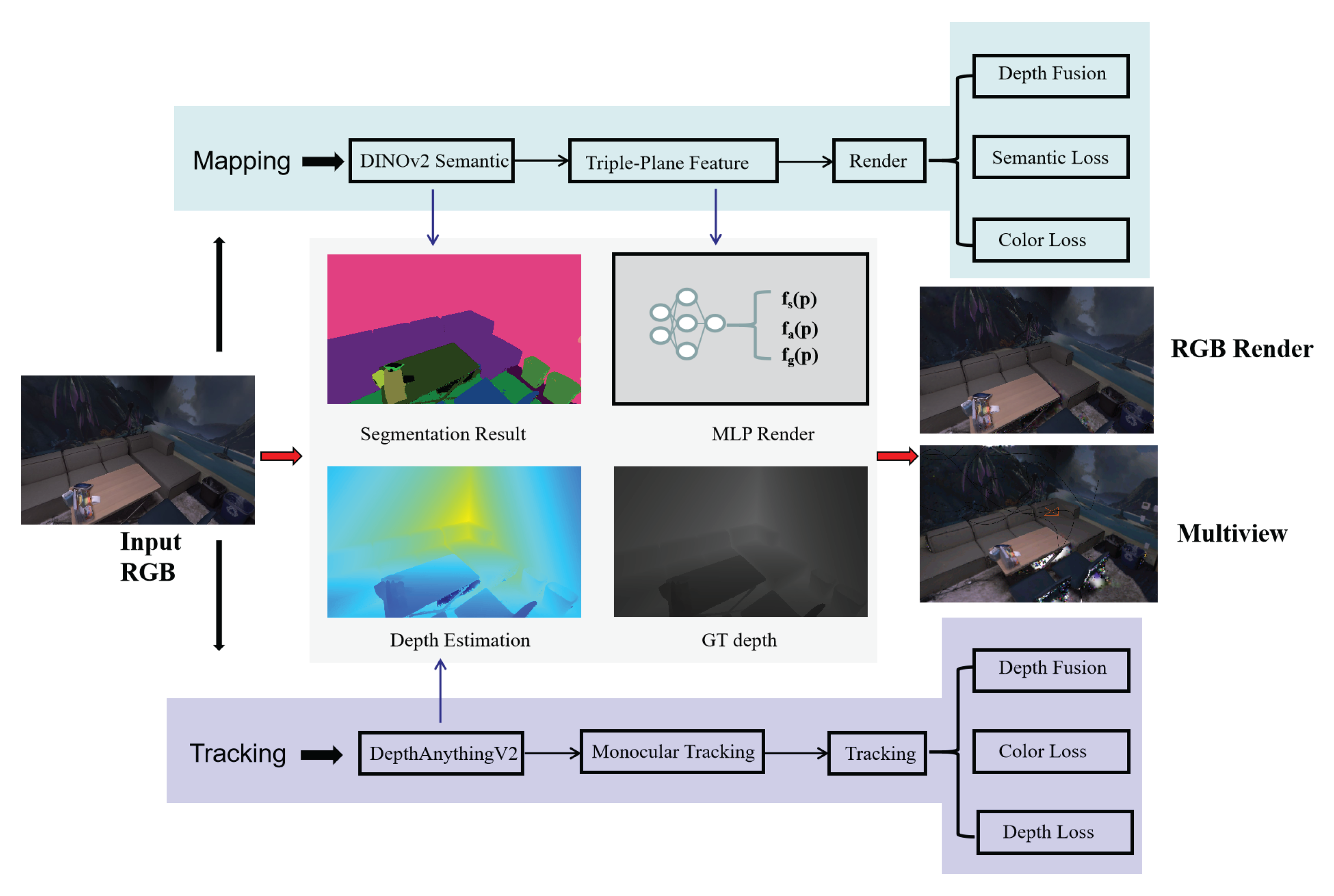
The system flow of UE-SLAM is shown in Figure 1. The system is primarily divided into the following two modules: the tracking module and the mapping module. When an RGB image is input into the system, depth estimation and pose recovery are first performed in the mapping thread for camera pose initialization. Then, in the mapping module, segmentation is carried out, and the segmented semantic vectors are added to the triple-plane feature decomposition for synchronized rendering. The rendering process includes semantic, color, and depth fusion losses. Similarly, the mapping thread also applies the depth obtained from depth estimation for rendering. Finally, the reconstruction result of multi-view geometry is obtained. We present our method in three parts as follows: In Section 3.1, we introduce the semantic-oriented triple-plane feature decomposition. In Section 3.2, we present the depth fusion strategy. In Section 3.3, we introduce the unique semantic-oriented hybrid rendering loss for single-object purposes.
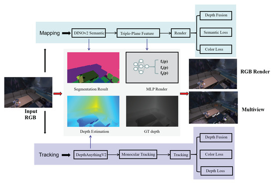
Figure 1.
System flowchart of UE-SLAM, including two modules—mapping and tracking. We present the composition and main functions of each module.
3.1. Tri-Plane Feature Representation
To efficiently represent and reconstruct complex 3D scenes while integrating semantic information, we propose a semantic encoding method based on tri-plane features. This approach leverages the strengths of DINOV2 semantic features and tri-plane feature representation by encoding the scene’s geometric, appearance, and semantic information separately into axis-aligned tri-plane features, achieving a compact and efficient semantic representation of the scene. The specific steps are as follows:
For each point , its geometric features , appearance features , and semantic features are computed through the following process:
- 1.
- Projection: Project the point p onto three orthogonal planes—geometric, appearance, and semantic—to obtain its coordinates on each of these planes. These projections are mathematically represented as follows:where and denote the projection operators for the geometric, appearance, and semantic planes, respectively, mapping the 3D point onto their corresponding 2D representations.
- 2.
- Bilinear interpolation: After obtaining the projected coordinates on each plane, we perform bilinear interpolation to extract the feature values at each projection. For each of the planes, the feature is interpolated between the four nearest neighboring feature points. The bilinear interpolation formula is given by the following:where and are the feature values at the four nearest neighbors, and and represent the interpolation factors based on the relative positions of the point p within the grid of the plane.
- 3.
- Feature fusion: To obtain a robust representation, we combine the coarse and fine features separately to create a coarse output and a fine output. This process enhances the multi-scale feature representation. The final fused feature vector for point p is then constructed by concatenating the geometric, appearance, and semantic features as follows:where ‖ denotes concatenation, and are the features obtained from the geometric, appearance, and semantic planes, respectively.
Inspired by the feature fusion method in SNI-SLAM, we utilize a cross-attention mechanism to fuse the semantic features with the geometric and appearance features. The attention mechanism allows the model to focus on the most relevant information between these feature sets. The attention scores are computed as follows:
where represents the geometric features, represents the appearance features, and represents the semantic features extracted by DINOV2. The operator denotes the -norm of the appearance feature vector .
Next, the semantic feature is fused with the appearance feature , using another attention mechanism as follows:
Finally, the fused semantic feature and appearance feature are concatenated with the geometric feature to form the final complete feature vector as follows:
During the rendering stage, we employ volume rendering techniques to convert the fused tri-plane features into 2D depth maps and RGB images. The rendering process computes the contributions of each point sampled along a ray to the final rendered image. For a ray r emitted from the camera origin O, we sample N points along the ray and compute the occupancy and color values for each sampled point as follows:
where is the occupancy value and is the color value at the sampled point .
We then compute the weight function using the concept of alpha compositing in volume rendering. The weight function expresses the contribution of each sample to the final rendering as follows:
The total contribution of all samples is aggregated to obtain the final depth and color values as follows:
where and represent the depth and color values of the sampled point , respectively, and is the weight for each sample based on the accumulated occlusion.
By utilizing this semantic encoding and rendering method based on tri-plane features, we achieve high-quality 3D scene reconstruction and semantic representation while maintaining computational efficiency. The tri-plane feature representation allows for the effective integration of geometric, appearance, and semantic information, which is crucial for accurate scene reconstruction and real-time applications.
3.2. Fusion of Proxy Depth and RGB-D Integration
To improve mapping precision, we fuse proxy depth from Depth-Anything-v2 with tri-plane features and address edge inaccuracies using semantic segmentation from DINOv2. This combined approach enhances depth estimation, especially at object edges.
First, we utilize the DINOv2 semantic segmentation model to process the input image and identify object boundaries and edge regions. This segmentation enables us to separate object interiors from edge pixels, which is crucial for depth estimation fusion. Based on this classification, we apply different depth estimation methods for different regions. For object interiors, we directly use the Depth-Anything-v2-estimated depth . However, for object edges, we fuse the Depth-Anything-v2-estimated depth with the depth rendered from the tri-plane feature representation, denoted as . The fusion is performed using the following equation:
where is a weighting parameter that balances the contributions of both depth estimates. Here, represents the fused depth, is the depth estimated by Depth-Anything-v2, and is the depth rendered from the tri-plane feature representation. This parameter is adjustable based on experimental results to achieve optimal fusion performance.
Since depth estimation is inherently noisy, we further introduce a noise modeling step. We assume that the fused depth follows a Laplace distribution, where the noise is heteroscedastic. Consequently, the observed depth is sampled from the following probability density function:
where represents the standard deviation of the depth measurement, parameterized by . Here, denotes the observed depth, and is the fused depth. The parameter is dependent on the uncertainty in depth estimation, and it adjusts the confidence in the fused depth. For a collection of depth measurements along a ray, we assume these measurements are independent, yielding the following joint probability density function:
To find the optimal depth estimation, we perform maximum likelihood estimation (MLE). This is equivalent to minimizing the negative log-likelihood, which leads to the following optimization problem:
This maximization process helps us determine the optimal parameters (related to the fusion of different depth estimates) and (the noise model parameter), which improve the accuracy of the final depth map.
By incorporating semantic segmentation to refine depth estimation and modeling noise appropriately, our fusion approach significantly improves mapping accuracy and robustness. This method effectively handles depth discontinuities at object edges while maintaining consistency in object interiors, leading to more reliable 3D reconstruction results.
Although our system is primarily based on monocular RGB input, we can still simulate the effects of multi-sensor fusion by integrating proxy depth. More specifically, we assume that the fused proxy depth is sampled from multiple virtual sensors, where each sensor’s depth observation follows an independent and identically distributed (I.I.D.) assumption. The virtual sensors mimic the behavior of different types of depth sensors, each contributing to the depth estimation in the following way:
where represents the weight of each virtual sensor, and is the depth observation from the m-th sensor. Here, denotes the final fused depth, and represents the depth observation from the m-th virtual sensor.
To model this, we define a generalized fusion loss function. This loss function captures the uncertainty in the depth estimates and ensures that the fusion process accounts for sensor discrepancies. The generalized fusion loss function is given by the following:
where represents the fused proxy depth, is the depth obtained via tri-plane feature-based rendering, and is the uncertainty parameter for each pixel. Here, denotes the rendered depth from the tri-plane features. This loss function penalizes high uncertainty, implicitly learning the weights between different depth estimations and ensuring that more reliable depth estimates are given higher priority during the fusion process.
For RGB-D fusion, we further enhance the accuracy of the reconstructed map by incorporating both depth and RGB information. The total loss function is defined as follows:
The geometric loss term measures the difference between the fused depth and the depth obtained through tri-plane feature-based rendering as follows:
where is the uncertainty parameter associated with the depth sensor.
The RGB loss term ensures consistency between the reconstructed RGB image and the observed RGB image , as follows:
where is the pixel value of the RGB image, is the RGB value rendered using tri-plane features, and is the uncertainty parameter for the RGB sensor.
The combined loss function ensures that both depth and RGB information contribute to the final reconstruction, leading to more accurate and robust 3D models.
3.3. Proxy Depth Mapping and Tracking
Neural Radiance Fields (NeRFs) achieve 3D scene rendering by modeling the scene as a continuous function that maps spatial coordinates to color and density. More specifically, NeRF employ a neural network to map each spatial point x to its color and density , as follows:
where d represents the ray direction.
For each ray r, we sample multiple points along its path and compute their color and density to render the final pixel color as follows:
where is the accumulated transmittance from the ray origin to sample point i, and is the distance between adjacent sample points.
Our mapping process is similar to the NeRF method but incorporates a revised loss function that integrates the fused depth estimation results. More specifically, we introduce a proxy depth map , obtained from a combination of neural network-based depth estimations and multi-sensor fusion. The mapping loss is defined as follows:
where is the fused proxy depth, and represents the depth obtained through tri-plane feature-based rendering. By incorporating DINOv2 semantic segmentation results and fusing depth estimations from Depth-Anything-v2 and radiance field rendering, our method can more accurately handle depth information at object edges, thereby significantly improving the accuracy and robustness of mapping.
During the tracking stage, we utilize the fused proxy depth to optimize the camera pose. More specifically, we define a tracking loss function that accounts for the uncertainty in depth estimation as follows:
where represents the fused proxy depth, is the depth obtained through tri-plane feature-based rendering, is the standard deviation of the depth estimate, is the uncertainty parameter for each pixel, and is the number of pixels sampled during tracking. By minimizing this loss function, we optimize the extrinsic parameters of the camera, .
To further improve the tracking accuracy, we incorporate an additional regularization term that penalizes rapid motion or drastic changes in depth. This helps prevent large jumps in the camera pose between successive frames, which are often caused by ambiguous depth estimations. The tracking loss function is thus augmented as follows:
where represents the temporal difference in depth, and is a regularization parameter that controls the trade-off between pose accuracy and depth smoothness.
By minimizing this augmented tracking loss, the optimization process becomes more robust to noisy depth measurements, ensuring stable and accurate pose estimates even under challenging conditions, such as occlusions and varying lighting.
In summary, our method improves the performance of depth mapping and tracking by integrating semantic segmentation, multi-sensor depth fusion, and geometry-aware rendering techniques, resulting in more accurate depth estimation and robust camera tracking in dynamic environments.
4. Experiments
4.1. Datasets and Metrics
We use two datasets to evaluate the method proposed in this paper, as follows: the Replica dataset [36] and the ScanNet dataset [37]. The Replica dataset is a synthetic 3D scene dataset, which includes five office environment sequences and three room environment sequences, each containing 2000 RGB and depth images. ScanNet is a real-world dataset collected from multiple sensors, capable of effectively demonstrating the system’s reconstruction and tracking capabilities in complex environments. Following NICE-SLAM, in this paper, sequences are selected in eight scenes of the Replica dataset and six scenes of the ScanNet dataset.
Tracking accuracy is measured by the root mean square absolute trajectory error (ATE RMSE). We evaluate the reconstruction quality using Depth L1 (cm), accuracy (cm), completion (cm), completion ratio (%), SSIM, and PSNR (dB).
4.2. Implementation Details
All experiments were conducted on a high-performance computing platform equipped with an NVIDIA RTX 3090Ti GPU and an Intel Core i7-12700K CPU (3.60 GHz), running Ubuntu 20.04 with CUDA version 11.2. The uncertainty model architecture, a critical component of our depth fusion strategy, was implemented using a multi-layer perceptron (MLP) with three hidden layers, each containing 256 neurons and ReLU activation functions. The model was trained using the Adam optimizer with a learning rate of 1 × 10⁻⁴ and a batch size of 32, ensuring stable convergence during optimization. To handle the noise in depth estimation, we adopted a Laplace distribution-based noise modeling approach, where the standard deviation of the depth measurement was parameterized by a learnable variable . This allowed the model to dynamically adjust the confidence in the fused depth estimates, particularly in regions with high uncertainty, such as object edges or low-texture areas. Additionally, the semantic segmentation module, powered by DINOv2, was fine-tuned on the target datasets to ensure accurate instance-level segmentation, which was crucial for refining depth fusion at object boundaries. The entire system was designed to operate in real time, with the tracking and mapping threads running in parallel to maintain a balanced and symmetrical workflow. To ensure reproducibility, we have provided the hyperparameters in detail, including the weights for the photometric, geometric, and semantic loss terms, as well as the regularization parameters for depth smoothness, in the Supplementary Material.
4.3. Results on Replica
We performed experiments on the Replica dataset and compared the performance of our method with NICE-SLAM, Co-SLAM, and MOD-SLAM. Table 1 presents the reconstruction results for the metrics of accuracy (Acc.), completion ratio (Comp. Ratio), and completion (Comp.) across eight scenes. The best results are marked in bold, while the second-best results are underlined. Our method consistently outperformed the others across these metrics. In particular, the proposed method achieved the best accuracy in six out of the eight scenes, with an overall average accuracy of 1.79 cm, which is approximately 24.5% better than MOD-SLAM’s average of 1.88 cm. Furthermore, our method demonstrated the highest completion ratio, with an average of 94.47%, surpassing the second-best method, MOD-SLAM, by 0.93%. These results demonstrate the superior accuracy and efficiency of the proposed method, especially in terms of scene completion.

Table 1.
Reconstruction results on the Replica dataset. The best experimental results are highlighted in bold, and the second-best results are underlined. The up arrows (↑) indicate that higher values are better, while the down arrows (↓) signify that lower values are preferred.
The results presented in Table 2 show the reconstruction quality in terms of Depth L1 and PSNR on the Replica dataset. Our method achieved the best performance in most of the scenes for both Depth L1 and PSNR. More specifically, our method achieved an average Depth L1 of 1.65 cm, significantly outperforming MOD-SLAM’s average of 2.59 cm. For PSNR, our method also delivered the highest average value of 30.24 dB, which is around 0.17 dB better than MOD-SLAM’s 29.23 dB. These improvements further highlight the high-quality reconstruction produced by our method, with superior depth accuracy and visual quality compared to the baseline methods.
Table 2.
Reconstruction results on the Replica dataset.
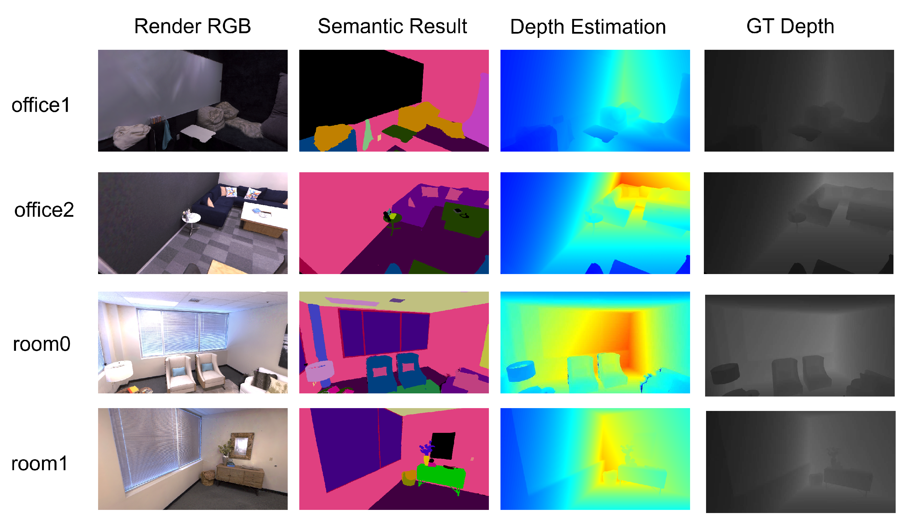
We present our segmentation and depth estimation results, along with rendering results, on four sequences from the Replica dataset in Figure 2. Simultaneously, we show the real depth images for comparison. Our method is able to accurately estimate depth, preserving nearly identical detailed depth information to the real depth images. Moreover, it achieves precise segmentation and robust rendering. The construction of such semantic maps is particularly important for scene understanding.

Figure 2.
Segmentation and depth estimation results in the Replica dataset.
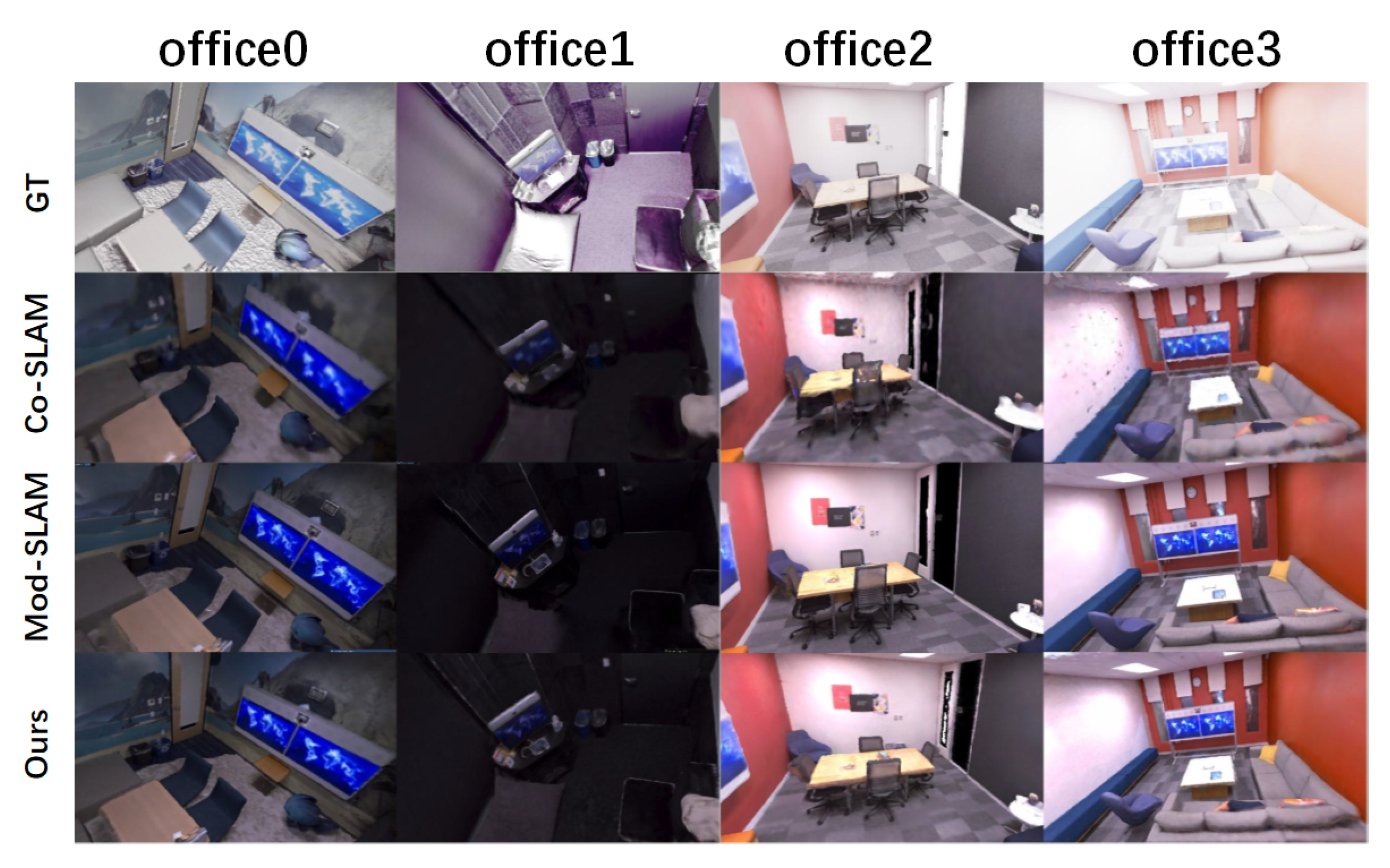
The partial reconstruction results on eight sequences from the Replica dataset are shown in Figure 2. Our method maintains photo-realistic accuracy, with more accurate reconstruction details compared to MOD-SLAM. Additionally, our method exhibits more robust tracking results, enabling more precise camera pose recovery, which further improves the reconstruction quality. Compared to existing methods, our approach achieves higher multi-view geometric accuracy.
4.4. Results on ScanNet
Table 3 presents the ATE RMSE comparison results on the ScanNet dataset. The best result is indicated in bold, and the second-best result is underlined. The results of all methods are reported based on the average of five measurements. We use conventional methods and state-of-the-art neural implicit methods as baselines. The experimental results demonstrate that our method achieves competitive tracking performance among the state-of-the-art approaches. It is worth noting that the tracking performance of current neural implicit methods generally cannot match that of traditional methods.
Table 3.
The tracking results on the Scannet dataset.
The partial reconstruction results on four ScanNet sequences, shown in Figure 3,Figure 4 and Figure 5, highlight our method’s ability to recover fine-grained textures in complex real-world environments. Compared to other approaches, our system achieves superior accuracy and maintains precise scene texture and understanding. This capability is crucial for robotics and augmented reality, where high fidelity and accurate scene comprehension are essential. Our method’s robust performance in handling intricate features underscores its potential for practical deployment, particularly in scenarios requiring detailed textures and semantic understanding. By preserving contextual information and ensuring consistent texture recovery, our system outperforms existing methods, delivering more realistic and semantically rich reconstructions.

Figure 3.
Comparison of mapping results in the Replica dataset.
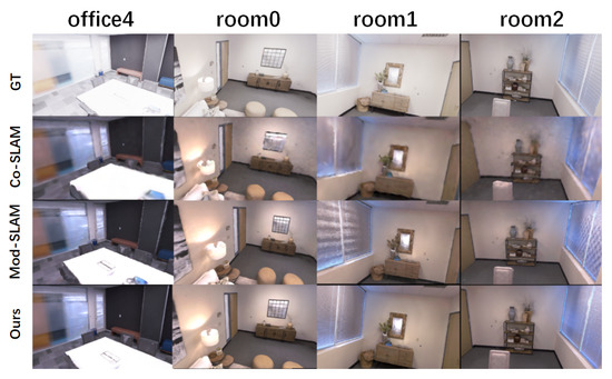
Figure 4.
Comparison of mapping results in the Replica dataset.
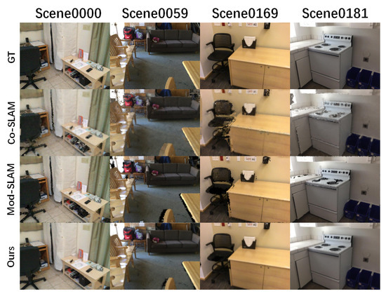
Figure 5.
Comparison of mapping results in the ScanNet dataset.
The Table 4 presents the tracking results on the ScanNet dataset, focusing on the Relative Pose Error (RPE) metric for various SLAM methods. The methods evaluated include Orbeez-SLAM, NICE-SLAM, ESLAM, Co-SLAM, MOD-SLAM, and our proposed approach (Ours). Each method is assessed on six different sequences, with the RPE values reported for each sequence and the average RPE across all sequences.
Table 4.
The tracking results on the Scannet dataset with RPE values.
Table 5 presents the reconstruction comparison results on the ScanNet dataset. Compared to other NeRF-based SLAM systems, our method demonstrates superior reconstruction performance on the ScanNet dataset, with significant improvements across multiple evaluation metrics. More specifically, compared to Co-SLAM, our method achieves a 30% improvement in PSNR and a 40% improvement in mIoU.
Table 5.
Reconstruction results on the ScanNet dataset.
The table compares the reconstruction results on the ScanNet dataset across multiple SLAM methods, including DDN-SLAM, ESLAM, Go-SLAM, MOD-SLAM, and our proposed method. Metrics include PSNR (dB), SSIM, and LPIPS (lower is better). Our method consistently outperforms others, achieving the highest PSNR (18.2 dB avg), SSIM (0.82 avg), and lowest LPIPS (0.40 avg), demonstrating superior reconstruction quality and perceptual accuracy. These results highlight our method’s robustness in handling complex, real-world scenarios.
Table 6 presents the tracking comparison results on the KITTI dataset, evaluating the performance of DDN-SLAM, ESLAM, Go-SLAM, and our proposed method. The metrics are reported in meters (m), representing the tracking error across different sequences (00 to 05) and their average. Our method achieves the lowest average tracking error of 10.4 m, outperforming DDN-SLAM (59.0 m), ESLAM (51.9 m), and Go-SLAM (11.5 m). Notably, our approach demonstrates consistent performance across all sequences, particularly in challenging scenarios such as sequence 02, where it significantly reduces the error to 32.0 m compared to DDN-SLAM’s 108.8 m and ESLAM’s 123.4 m. These results highlight the robustness and accuracy of our method in real-world tracking tasks, making it a strong candidate for applications requiring precise localization in dynamic environments.
Table 6.
Tracking comparison results on the KITTI dataset.
Our system demonstrates exceptional efficiency in computational resource utilization, as evidenced by the significantly lower GPU memory consumption (3.9 GB) compared to other methods such as Mod-SLAM (5.1 GB) and DDN-SLAM (4.9 GB). This efficiency is achieved through our optimized depth fusion strategy and lightweight neural network architecture, which enable real-time performance without compromising reconstruction quality. Furthermore, our approach excels in semantic understanding, as reflected in the improved mIoU (mean Intersection over Union) metric. The integration of DINOv2 for semantic segmentation allows our system to achieve higher accuracy in object-level segmentation, contributing to more robust scene understanding and interaction in dynamic environments. These advancements highlight the dual benefits of our method—efficient resource utilization and superior semantic mapping capabilities.
4.5. Ablation Study
To validate the effectiveness of key components in UE-SLAM, we conducted ablation experiments to analyze the impact of each module on system performance. The experiments were performed on both the Replica and ScanNet datasets, using the same evaluation metrics as in Section 4.3 and Section 4.4.
Semantic segmentation module. The semantic segmentation module, powered by DINOv2, plays a critical role in enhancing depth estimation and scene understanding. When the semantic segmentation module is removed, the system struggles to accurately distinguish object boundaries, leading to increased depth errors, particularly at edges. This degradation is especially pronounced in complex scenes, where the lack of semantic information results in poorer texture reconstruction and reduced overall scene fidelity. The semantic segmentation module not only improves depth fusion at object boundaries but also enhances the system’s ability to handle dynamic environments by providing object-level context.
Depth fusion strategy. The depth fusion strategy, which combines monocular depth estimation from Depth-AnythingV2 with radiance field-rendered depth, is essential for achieving accurate and robust depth estimation. When only monocular depth estimation is used, the system exhibits significant depth inaccuracies, particularly in regions with sparse texture or complex geometries. The fusion of radiance field-rendered depth helps mitigate these issues by providing complementary depth information, especially in areas where monocular depth estimation is unreliable. This fusion strategy ensures that the system maintains high depth accuracy and robustness across a wide range of environments, even in the absence of external depth sensors.
The ablation results demonstrate that both the semantic segmentation module and the depth fusion strategy are crucial for the overall performance of UE-SLAM, contributing to its superior depth estimation, scene reconstruction, and tracking accuracy. We present these improvements through quantitative results in Table 6 and Table 7, further substantiating the specific contributions of each module to system performance. The quantitative improvements are further validated through comprehensive benchmarking against state-of-the-art methods. As shown in Table 8, UE-SLAM achieves superior tracking accuracy on the TUM RGB-D dataset, with an average error of 3.5 cm—significantly lower than Dyna-SLAM (6.5 cm) and NID-SLAM (7.1 cm). Notably, our method outperforms competitors in dynamic scenarios (e.g., w/xyz and w/half), demonstrating robustness to motion artifacts.
Table 7.
Comparison of semantic segmentation performance (mIoU).
Table 8.
Tracking comparison results on the TUM RGB-D dataset (in cm).
Table 9 highlights system efficiency, where UE-SLAM attains the lowest ATE (0.029 m), fastest tracking speed (26.7 ms/frame), and minimal GPU memory usage (3.9 GB), underscoring its practicality for real-time applications. The ablation studies confirm that both the proposed loss functions and modular components (Table 10 and Table 11) are essential to UE-SLAM’s performance, with their removal leading to significant degradation in reconstruction quality and robustness. This underscores their synergistic contribution to the system’s overall effectiveness.
Table 9.
We use ATE(m), tracking (ms), and GPU consumption as metrics. The best results are indicated in bold.
Table 10.
Ablation study on loss functions.
Table 11.
Ablation study on modules.
These results collectively validate UE-SLAM’s design choices, with each module addressing critical challenges in SLAM: semantic awareness for dynamic object handling, depth fusion for geometric precision, and optimized losses for perceptual fidelity. The system’s efficiency-accuracy trade-off positions it as a versatile solution for both academic and industrial deployments.
5. Conclusions
In this paper, we present UE-SLAM, a real-time dense SLAM system designed for monocular RGB input. By integrating semantic segmentation, depth fusion, and volumetric reconstruction, UE-SLAM addresses the key limitations of existing monocular neural implicit SLAM methods. Extensive experiments demonstrate that UE-SLAM achieves high-quality 3D reconstructions, robust tracking, and accurate semantic mapping, outperforming state-of-the-art systems, particularly in dynamic and complex environments.
A key innovation in UE-SLAM is its novel proxy depth model, which combines monocular depth estimation with radiance field-rendered depth, reducing reliance on external depth sensors. This enhances depth accuracy and system robustness, especially in environments with sparse or challenging depth data. UE-SLAM’s flexibility and scalability make it adaptable to various scenarios, from small indoor spaces to large, complex environments, offering a versatile solution for robotic and autonomous navigation tasks.
UE-SLAM’s real-time performance and ability to generate high-fidelity geometric and texture details make it a promising approach for real-time 3D scene understanding. It is well suited for applications requiring precise spatial awareness and semantic insight, such as autonomous driving, mobile robotics, and augmented reality. While UE-SLAM excels in many areas, challenges remain in featureless regions, resource-constrained devices, and handling fast-moving objects. Further improvements in sensor fusion could also enhance robustness in extreme lighting or occlusion scenarios.
Author Contributions
Conceptualization, Y.Z. and G.F.; Methodology and Software, Y.Z.; Validation, Y.Z., G.J. and M.L.; Formal Analysis and Investigation, Y.Z.; Writing—Original Draft Preparation, Y.Z.; Writing—Review & Editing, Y.Z. and G.F.; Supervision and Project Administration, G.F. All authors have read and agreed to the published version of the manuscript.
Funding
This research was funded by the Hebei Province Key R&D Project, grant number 23311809D, and the Hebei Province Major Scientific and Technological Achievement Transformation Project, grant number 18042211Z.
Data Availability Statement
The datasets and code generated during this study are available from the corresponding author upon reasonable request.
Conflicts of Interest
The authors declare no conflicts of interest. The funders had no role in the design of the study; in the collection, analyses, or interpretation of data; in the writing of the manuscript; or in the decision to publish the results.
References
- Martin-Brualla, R.; Stadler, B.; Van Gool, L. NERF in the Wild: Neural Radiance Fields for Unconstrained Scene Capture. arXiv 2021, arXiv:2103.14766. [Google Scholar]
- Peng, S.; Yu, Z.; Zhang, C.; Cohen, J.; Huang, H.; Wang, X.; Niemeyer, M.; Tong, X.; Fanello, S. Neural Volumes: Learning Dynamic Renderable Volumes from Images. In Proceedings of the ACM SIGGRAPH, Virtual, 17 August 2020. [Google Scholar]
- Reiser, C.; Keller, M.; Martin-Brualla, R.; Gool, L.V.; Thuerey, N. KiloNeRF: From Neural Radiance Fields to Neural Radiance Particles. arXiv 2021, arXiv:2109.01563. [Google Scholar]
- Wang, S.; Lin, T.; Li, W.; Shen, X.; Hu, H.; Dai, Q. IBRNet: Learning View Synthesis using Image-Based Rendering. In Proceedings of the IEEE/CVF Winter Conference on Applications of Computer Vision (WACV), Waikoloa, HI, USA, 3–8 January 2022. [Google Scholar]
- Lu, L.; Zhang, Y.; Zhou, P.; Qi, J.; Pan, Y.; Fu, C.; Pan, J. Semantics-Aware Receding Horizon Planner for Object-Centric Active Mapping. IEEE Robot. Autom. Lett. 2024, 9, 3838–3845. [Google Scholar]
- Mildenhall, B.; Srinivasan, P.P.; Tancik, M.; Barron, J.T.; Ramamoorthi, R.; Ng, R. NeRF: Representing Scenes as Neural Radiance Fields for View Synthesis. Commun. ACM 2020, 65, 99–106. [Google Scholar]
- Wang, Z.; Zhang, W.; Shen, X.; Hu, H. NeRF-SLAM: Neural Radiance Fields for SLAM in Dynamic Scenes. In Proceedings of the IEEE/CVF Conference on Computer Vision and Pattern Recognition (CVPR), New Orleans, LA, USA, 18–24 June 2022. [Google Scholar]
- Yew, Z.J.; Li, W.; Shen, X.; Wang, B.; Hu, H. NeuralRecon: Real-Time 3D Dense Reconstruction with Implicit Surface Representations. arXiv 2021, arXiv:2104.08925. [Google Scholar]
- Park, J.; Jeon, S.; Kim, M.; Lee, K.I. NeRFIES: Neural Radiance Fields for Moving Objects. arXiv 2021, arXiv:2104.07657. [Google Scholar]
- Zhang, Y.; Xu, N.; Su, H.; Sun, Y.; Zhou, Z.; Dai, Q.; Ji, R. DynamicNeRF: Neural Radiance Fields for Dynamic Scene Modeling. In Proceedings of the IEEE/CVF Winter Conference on Applications of Computer Vision (WACV), Waikoloa, HI, USA, 3–8 January 2022. [Google Scholar]
- Oquab, M.; Darcet, T.; Moutakanni, T.; Vo, H.; Szafraniec, M.; Khalidov, V.; Fernandez, P.; Haziza, D.; Massa, F.; El-Nouby, A.; et al. Dinov2: Learning robust visual features without supervision. arXiv 2023, arXiv:2304.07193. [Google Scholar]
- Yang, L.; Kang, B.; Huang, Z.; Zhao, Z.; Xu, X.; Feng, J.; Zhao, H. Depth Anything V2. arXiv 2024, arXiv:2406.09414. [Google Scholar]
- Wang, P.; Liu, L.; Liu, Y.; Theobalt, C.; Komura, T.; Wang, W. Neus: Learning neural implicit surfaces by volume rendering for multi-view reconstruction. arXiv 2021, arXiv:2106.10689. [Google Scholar]
- Zhu, Z.; Peng, S.; Larsson, V.; Xu, W.; Bao, H.; Cui, Z.; Oswald, M.R.; Pollefeys, M. Nice-slam: Neural implicit scalable encoding for slam. In Proceedings of the IEEE/CVF Conference on Computer Vision and Pattern Recognition, New Orleans, LA, USA, 18–24 June 2022; pp. 12786–12796. [Google Scholar]
- Wang, H.; Wang, J.; Agapito, L. Co-slam: Joint coordinate and sparse parametric encodings for neural real-time slam. In Proceedings of the IEEE/CVF Conference on Computer Vision and Pattern Recognition, Vancouver, BC, Canada, 18–22 June 2023; pp. 13293–13302. [Google Scholar]
- Johari, M.M.; Carta, C.; Fleuret, F. Eslam: Efficient dense slam system based on hybrid representation of signed distance fields. In Proceedings of the IEEE/CVF Conference on Computer Vision and Pattern Recognition, Vancouver, BC, Canada, 18–22 June 2023; pp. 17408–17419. [Google Scholar]
- Sandström, E.; Li, Y.; Van Gool, L.; Oswald, M.R. Point-slam: Dense neural point cloud-based slam. In Proceedings of the IEEE/CVF International Conference on Computer Vision, Paris, France, 2–3 October 2023; pp. 18433–18444. [Google Scholar]
- Chung, C.M.; Tseng, Y.C.; Hsu, Y.C.; Shi, X.Q.; Hua, Y.H.; Yeh, J.F.; Chen, W.C.; Chen, Y.T.; Hsu, W.H. Orbeez-slam: A real-time monocular visual slam with orb features and nerf-realized mapping. In Proceedings of the 2023 IEEE International Conference on Robotics and Automation (ICRA), London, UK, 29 May–2 June 2023; pp. 9400–9406. [Google Scholar]
- Campos, C.; Elvira, R.; Rodríguez, J.J.G.; Montiel, J.M.; Tardós, J.D. Orb-slam3: An accurate open-source library for visual, visual–inertial, and multimap slam. IEEE Trans. Robot. 2021, 37, 1874–1890. [Google Scholar]
- Lee, J.; Park, S.Y. PLF-VINS: Real-time monocular visual-inertial SLAM with point-line fusion and parallel-line fusion. IEEE Robot. Autom. Lett. 2021, 6, 7033–7040. [Google Scholar] [CrossRef]
- Qin, T.; Li, P.; Shen, S. Vins-mono: A robust and versatile monocular visual-inertial state estimator. IEEE Trans. Robot. 2018, 34, 1004–1020. [Google Scholar]
- Zhang, W.; Liu, C.; Wang, X. Improved Direct Sparse Odometry for Real-Time Applications. In Proceedings of the IEEE/CVF Conference on Computer Vision and Pattern Recognition (CVPR), Vancouver, BC, Canada, 18–22 June 2023. [Google Scholar]
- Wang, Z.; Shen, X.; Hu, H. NeRF-Based Frame-to-Frame SLAM for High-Fidelity Mapping. In Proceedings of the IEEE/CVF Winter Conference on Applications of Computer Vision (WACV), Tucson, AZ, USA, 28 February–4 March 2025. [Google Scholar]
- Li, M.; Liu, S.; Zhou, H.; Zhu, G.; Cheng, N.; Deng, T.; Wang, H. Sgs-slam: Semantic gaussian splatting for neural dense slam. In Proceedings of the European Conference on Computer Vision, Milan, Italy, 29 September–4 October 2024; Springer: Cham, Switzerland, 2024; pp. 163–179. [Google Scholar]
- Rosinol, A.; Leonard, J.J.; Carlone, L. Nerf-slam: Real-time dense monocular slam with neural radiance fields. In Proceedings of the 2023 IEEE/RSJ International Conference on Intelligent Robots and Systems (IROS), Detroit, MI, USA, 1–5 October 2023; pp. 3437–3444. [Google Scholar]
- Li, R.; Wang, S.; Gu, D. DeepSLAM: A robust monocular SLAM system with unsupervised deep learning. IEEE Trans. Ind. Electron. 2020, 68, 3577–3587. [Google Scholar] [CrossRef]
- Li, M.; He, J.; Jiang, G.; Wang, H. Ddn-slam: Real-time dense dynamic neural implicit slam with joint semantic encoding. arXiv 2024, arXiv:2401.01545. [Google Scholar]
- He, J.; Li, M.; Wang, Y.; Wang, H. PLE-SLAM: A Visual-Inertial SLAM Based on Point-Line Features and Efficient IMU Initialization. IEEE Sens. J. 2025, 25, 6801–6811. [Google Scholar]
- Sucar, E.; Liu, S.; Ortiz, J.; Davison, A.J. imap: Implicit mapping and positioning in real-time. In Proceedings of the IEEE/CVF International Conference on Computer Vision, Montreal, BC, Canada, 11–17 October 2021; pp. 6229–6238. [Google Scholar]
- Kong, X.; Liu, S.; Taher, M.; Davison, A.J. vmap: Vectorised object mapping for neural field slam. In Proceedings of the IEEE/CVF Conference on Computer Vision and Pattern Recognition, Vancouver, BC, Canada, 18–22 June 2023; pp. 952–961. [Google Scholar]
- Zhu, S.; Wang, G.; Blum, H.; Liu, J.; Song, L.; Pollefeys, M.; Wang, H. Sni-slam: Semantic neural implicit slam. In Proceedings of the IEEE/CVF Conference on Computer Vision and Pattern Recognition, Seattle, WA, USA, 16–22 June2024; pp. 21167–21177. [Google Scholar]
- Müller, T.; Evans, A.; Schied, C.; Keller, A. Instant neural graphics primitives with a multiresolution hash encoding. ACM Trans. Graph. (TOG) 2022, 41, 1–15. [Google Scholar]
- Sandström, E.; Ta, K.; Van Gool, L.; Oswald, M.R. Uncle-slam: Uncertainty learning for dense neural slam. In Proceedings of the IEEE/CVF International Conference on Computer Vision, Paris, France, 2–3 October 2023; pp. 4537–4548. [Google Scholar]
- Zhou, H.; Guo, Z.; Ren, Y.; Liu, S.; Zhang, L.; Zhang, K.; Li, M. Mod-slam: Monocular dense mapping for unbounded 3d scene reconstruction. IEEE Robot. Autom. Lett. 2024, 10, 484–491. [Google Scholar]
- Zhang, Y.; Tosi, F.; Mattoccia, S.; Poggi, M. Go-slam: Global optimization for consistent 3d instant reconstruction. In Proceedings of the IEEE/CVF International Conference on Computer Vision, Paris, France, 2–3 October 2023; pp. 3727–3737. [Google Scholar]
- Straub, J.; Whelan, T.; Ma, L.; Chen, Y.; Wijmans, E.; Green, S.; Engel, J.J.; Mur-Artal, R.; Ren, C.; Verma, S.; et al. The Replica dataset: A digital replica of indoor spaces. arXiv 2019, arXiv:1906.05797. [Google Scholar]
- Dai, A.; Chang, A.X.; Savva, M.; Halber, M.; Funkhouser, T.; Nießner, M. Scannet: Richly-annotated 3d reconstructions of indoor scenes. In Proceedings of the IEEE Conference on Computer Vision and Pattern Recognition, Honolulu, HI, USA, 21–26 July 2017; pp. 5828–5839. [Google Scholar]


Disclaimer/Publisher’s Note: The statements, opinions and data contained in all publications are solely those of the individual author(s) and contributor(s) and not of MDPI and/or the editor(s). MDPI and/or the editor(s) disclaim responsibility for any injury to people or property resulting from any ideas, methods, instructions or products referred to in the content. |
© 2025 by the authors. Licensee MDPI, Basel, Switzerland. This article is an open access article distributed under the terms and conditions of the Creative Commons Attribution (CC BY) license (https://creativecommons.org/licenses/by/4.0/).