Abstract
In one of our previous papers, we obtained a general class of potentials inside the nucleus, such that the singular solution of the Dirac equation for the S-states of hydrogen atoms outside the nucleus can be matched with the corresponding regular solution inside the nucleus (the proton) at the boundary. The experimental charge density distribution inside the proton generates a particular case of such potentials inside the proton. In this way, the existence of the second kind of hydrogen atom was predicted: atoms having only S-states. This theoretical prediction was then evidenced by several different types of atomic experiments and by astrophysical observations. In the present paper we provide the following new results. First, we show that the solution of the Dirac equation inside the proton can be (and is) found within the class of functions that are non-analytic at r = 0—in distinction to the traditional practice of limiting the search for the solution by the class of analytic functions. We demonstrate that this non-analytic solution inside the proton can be matched at the proton boundary R with the corresponding singular solution outside the proton regardless of the particular value of R. Second, we show that the interior and exterior solutions are scale-invariant with respect to the change of the boundary R between these two regions. Such invariance is the manifestation of a new symmetry—in addition to the previously discussed symmetries of the Dirac equation in the literature. Third, based on the new, more accurate results for the wave function inside and outside the proton, we revisit the resolution of the neutron lifetime puzzle initially outlined in our previous papers. On the basis of the more accurate calculations, we reconfirm that (A) the 2-body decay of neutrons produces overwhelmingly the SFHA (rather than the usual hydrogen atoms) and (B) the strengthened-in-this-way branching ratio for the 2-body decay of neutrons (compared to the 3-body decay) is in excellent agreement with the branching ratio required for reconciling the neutron lifetime values measured in the trap and beam experiments, so that the neutron lifetime puzzle seems to be indeed resolved in this way.
1. Introduction
There was a long-standing huge disagreement between the experimental [1] and theoretical [2] results concerning one of the features of hydrogen atoms: the Distribution of the Linear Momentum (DLM) in the lowest (ground) state. Namely, for relatively large momenta p, the theoretical DLM decreased much more rapidly than the experimental DLM, the ratio of the two reaching tens of thousands.
In paper [3], this discrepancy was resolved by engaging the second solution of the Dirac equation, for which the corresponding radial wave function R0,−1 (r) is proportional (at relatively small r) to 1/r q with q = 1 + (1 − α2)1/2, α being the fine structure constant (The second subscript of the wave function R0,−1 is the eigenvalue of the operator K = b(2Ls +1), which is the conserved quantity. Here, L is the orbital angular momentum, s is the spin, and b is the Dirac matrix 4 × 4). In paper [3], it was shown that after allowing for the finite size of the proton and for the fact that the charge density distribution inside the proton has the maximum at the origin and then decreases toward the proton periphery, the second solution becomes legitimate—because at the proton boundary, both the interior solution and the second exterior solution, as well as their derivatives, are continuous, as required by quantum mechanics.
The central point was the following. The much more robust increase of the second exterior wave function toward the proton boundary compared to the first exterior wave function corresponded—in the momentum representation—to the significantly more moderate decrease of the second exterior wave function for large momenta compared to the 1st exterior wave function, according to the Fourier transform properties. As a result, the long-standing huge disagreement between the experimental and theoretical results concerning the DLM was totally removed.
Later, in paper [4], it was noted that the legitimacy of the second exterior solution in paper [3] was based on the fact that the quantum number k (shown as the second subscript of R0,−1 (r)) was equal to −1. For this reason, the second exterior solution of the Dirac equation is legitimate for any state (of hydrogen atoms) characterized by k = −1. The states of k = −1 are the S-states, i.e., the states of zero orbital momentum.
This second kind of hydrogen atom, which does not have states of the non-zero orbital momentum, was called the Second Flavor of Hydrogen Atoms (SFHA) in a subsequent paper [5]. This is because both the first and second exterior solutions correspond to the same energy: consequently, the additional degeneracy—consequently, an additional conserved quantity—consequently, the flavor symmetry (just as in the case of quarks).
The above solution of the DLM puzzle, together with the absence of any alternative explanation, represented the 1st experimental evidence that the SFHA exists. By now there are several pieces of additional experimental/observational evidence regarding the existence of the SFHA, as follows.
The experimental [6,7,8] and theoretical [9] cross sections of the excitation of the triplet states of the H2 molecule by the electron impact showed a disagreement of 3 to 5 times. The possible presence of the SFHA in the experimental gas removed this disagreement [10], while no alternative explication was given.
The experimental [11,12] and theoretical [13] cross sections of the excitation of the 2S state of hydrogen atoms by the electron impact demonstrated a disagreement of 20% (while the error margins were just 9%). The possible presence of the SFHA in the experimental gas removed this disagreement [14], while no alternative explication was given.
One of the primary latest applications of the SFHA is in resolving the neutron lifetime puzzle, as briefly presented in paper [15]. The puzzle was the following.
In the experiments using the beam technique, the measured neutron lifetime τbeam turned out to be greater than the neutron lifetime τtrap measured in the experiments using the trap technique, significantly beyond the margins of error (see, e.g., paper [16] and the references therein). The primary channel of limiting the neutron lifetime is the 3-body decay, producing a proton, an electron, and an antineutrino. In the beam experiments, there were counted only the protons from the 3-body decay. Theoretically, there should be also the 2-body decay producing a hydrogen atom and an antineutrino. To explain the neutron lifetime puzzle via 2-body decay, missed in the beam experiments, it would require the branching ratio (BR) for the 2-body decay (with respect to the 3-body decay) to be ~1%. However, from paper [17] of 1961, it was known that the corresponding BR is just 4 × 10⁻⁶.
In paper [15], there was outlined that the 2-body decay of neutrons should produce overwhelmingly the SFHA rather than the usual hydrogen atoms. It was roughly estimated that this can increase the corresponding BR to ~1%, which would resolve the puzzle. We note that paper [15] was focused primarily on neutron stars, so that the 2-body decay of neutrons was just a “by-product” presented sketchily.
The most important feature of the SFHA is that, because of having only S-states, and in view of the selection rules of quantum mechanics, the SFHA does not couple to the electromagnetic radiation, including the dipole and higher multipole radiation, as well as multi-photon transitions. The SFHA cannot be excited or ionized by a static electric field or by a laser field, though it can be excited or ionized, e.g., by an electron beam.
In connection with the above most important feature of the SFHA, let us briefly reiterate astrophysical evidence of the existence of the SFHA. Bowman et al. [18], while observing the 21 cm line from the early Universe, found that the absorption signal in this line is 2 to 3 times stronger than expected from standard cosmology, meaning that the primordial hydrogen gas was significantly cooler than expected. The most plausible cooling agent was some unspecified baryonic dark matter (DM) particles that cooled the hydrogen gas by collisions—first according to Barcana [19] and then confirmed by McGaugh [20]. Then, in paper [4], it was shown that if the role of the unspecified baryonic DM particles was played by the SFHA, then this would explain the perplexing observation made by Bowman et al. [18], not only qualitatively, but also quantitatively; this made the SFHA a compelling candidate for being the baryonic DM.
Moreover, the comparison of the observed cosmological data on the ratio of the total DM to the usual matter and on the ratio of baryonic DM to non-baryonic DM with the data from atomic experiments that evidenced the existence of the SFHA, led to the following conclusion. The SFHA seems to comprise most of the baryonic DM in the current epoch [21].
It is significant that the SFHA is established as the solution of the Dirac equation, i.e., within the standard quantum mechanics. Thus, first, it is within the Standard Model of particle physics and second, no change of the physical laws is required. This is the clear difference of the SFHA compared to the vast majority of the models of DM (For completeness, we note the possibility of the existence of the second flavor of heavy hydrogenic ions, whose nuclei are doubly-magic and therefore spherical—as presented in our previous paper [22]).
In the present paper, we provide the following new results. First, we derive the explicit form of the solution of the Dirac equation inside the proton for the S-states—the solution that at the proton boundary matches the corresponding singular solution, as required by quantum mechanics—both the wave function and its derivative are continuous at the boundary. We show that such a solution inside the proton can be (and is) found within the class of functions that are non-analytic at r = 0—in distinction to the traditional practice of limiting the search for the solution by the class of analytic functions, i.e., by functions that can be adequately represented by their expansion into the Laurent series.
Second, we show that the interior and exterior solutions are scale-invariant with respect to the change of the boundary R between these two regions. Such invariance is the manifestation of a new symmetry—in addition to the previously discussed symmetries of the Dirac equation in the literature (see, e.g., papers [23,24,25,26,27,28] and the references therein).
Third, based on the new, more accurate results for the wave function inside and outside the proton, we revisit the resolution of the neutron lifetime puzzle initially outlined in our paper [15]. On the basis of the more accurate calculations, we reconfirm that the 2-body decay of neutrons produces overwhelmingly the SFHA (rather than the usual hydrogen atoms). Further, we reconfirm that the strengthened-in-this-way branching ratio for the 2-body decay of neutrons (compared to the 3-body decay) is in excellent agreement with the branching ratio required for reconciling the neutron lifetime values measured in the trap and beam experiments. In other words, our new, more accurate results for the wave function inside and outside the proton enhance the reliability of this resolution of the neutron lifetime puzzle.
In Appendix A, we offer details on the experimental charge distribution inside the proton.
2. Analytic Solution of the Dirac Equation Inside the Proton for the S-States of Hydrogen Atoms
For hydrogen atoms, the Dirac equation for the f- and g-components of the Dirac bispinor has the form (in the natural units ħ = me = c = 1)—see, e.g., textbook [29]:
where
df(r)/dr = (k − 1)f(r)/r − h1(r)g(r),
dg(r)/dr = h2(r)f(r) − (k + 1)g(r)/r,
h1(r) = W − 1 − V(r), h2(r) = W + 1 − V(r).
In Equation (3), W is the energy and V(r) is the potential energy of the atomic electron. In Equations (1) and (2)), k is the eigenvalue of the operator K = b(2Ls +1) mentioned in the Introduction.
For the S-states (on which we focus in the present paper), k = −1. Then, from Equation (2) we find:
f(r) = [dg(r)/dr]/h2(r).
On substituting Equation (4) in Equation (1), we obtain:
r(d2g/dr2) + [2 + r(dV/dr)/h2(r)](dg/dr) + rh1(r)h2(r)g = 0.
Now, we study this equation and its solution near the origin, i.e., near r = 0. After denoting
V0 = −|V(0)| = const > 0,
Equations (4) and (5) can be simplified as follows:
where
r[d2g(r)/dr2) + 2[dg(r)/dr] + hrg(r) = 0,
f(r) = [dg(r)/dr]/h20,
h = (W + V0)2 − 1 = const,
h20 = W + 1 +V0 = const.
We start from the traditional practice of limiting the search for the solutions by the class of analytic functions, i.e., by functions that can be adequately represented by their expansion into the Laurent series. Namely, we seek the solutions in the form:
where am = const for any n and d = const. On substituting Equation (11) into Equation (7) and requesting the mutual cancellation of the lowest powers of r, we find:
so that d1 = 0 and d2 = −1.
d(d + 1) = 0,
For the solution with d1 = 0, corresponding to
from Equation (8) we get:
g1(r) ≈ a0,
f1(r) ≈ a1/h20.
For the solution with d2 = –1, corresponding to
from Equation (8) we obtain:
g2(r) ≈ a0/r,
f2(r) ≈ −a0/( h20r2).
The normalization integral is
It is easy to see that for the solution with d = −1, the normalization integral diverges at r = 0, so that this solution should be rejected. For the solution with d = 0, the normalization integral converges at r = 0, so that this solution should be accepted.
3. Non-Analytic Solution of the Dirac Equation Inside the Proton for the S-States of Hydrogen Atoms
Non-analytic solutions of differential equations have been studied for many years—see, e.g., papers [30,31,32,33,34,35,36] listed in reversed chronological order. Here, we seek a non-analytic solution for the “interior” Equation (7) in the form:
where R is the matching radius, i.e., the radius at which the interior solution should be matched with the singular exterior solution.
gint(r) = (1/rγ)exp[−(R/r)β], β = const > 0, γ = const,
It is important to note that this class of solutions embraces the traditional class of analytical solutions as a particular case of β = 0. Thus, this class of solutions constitutes the generalization of the traditional class of analytical solutions.
Obviously, the function gint(r) from Equation (18) satisfies Equation (7) at r → 0. Then, according to Equation (8):
fint(r) = [−γ/rγ+1 +βRβ/rγ+1+β]exp[−(R/r)β]/h20.
For the exterior solution, the potential energy of the atomic electron is (in the natural units)
V(r) = −α/r,
α being the fine structure constant. Since the energy of the states of the principal quantum number n is approximately
then h1(r) and h2(r) from Equation (3) can be approximated as follows:
W ≈ 1 − α2/(2n2), n = 1, 2, 3, … .
h1(r) ≈ α/r − α2/(2n2), h2(r) ≈ α/r + 2.
For the range of r such that
h1(r) and h2(r) can be further simplified to
R ≤ r << 2/α,
h1(r) ≈ α/r, h2(r) ≈ α/r.
After taking into account Equations (20) and (24), the exterior solution should satisfy the Dirac equation in the following form:
r(d2g/dr2) + 3(dg/dr) + (α2/r)g = 0.
We seek the solution of the “exterior” Equation (25) expressed as
gext(r) = Crδ, C = const.
On substituting Equation (26) in Equation (25), we get the following equation:
δ2 + 2δ + α2 = 0.
Equation (27) has two solutions:
δ1 = (1 − α2)1/2 − 1 ≈ − α2/2, δ2 = − (1 − α2)1/2 − 1 ≈ − 2.
For the first solution (which we call “regular”):
gext(r) ≈ C/rε, fext(r) ≈ −αC/(2rε), ε = α2/2 ≈ 2.66 × 10⁻⁵ << 1.
For the second solution (which we call “singular”):
gext(r) ≈ C/r2, fext(r) ≈ −2C/(αr2).
In Equations (29) and (30), for deriving f(r) from g(r), we used Equations (4) and (23). The expressions for gext(r) from Equations (29) and (30) reproduce the well-known “small r” results of solving the Dirac equation for the Coulomb potential—see, e.g., textbook [30].
Now, we proceed by matching the singular gext(r) and fext(r) from Equation (30), as well as the logarithmic derivatives of these functions, with the corresponding interior solutions from Equations (18) and (19) at r = R. Equating the interior and exterior logarithmic derivatives of the g-component yields
so that
−(γ − β)/R = −2/R,
γ = β + 2.
Equating the interior and exterior logarithmic derivatives of the f-component and taking into account Equation (32) yields
so that
−(3 − β2/2)/R = −2/R,
β = 21/2.
Thus, the explicit form of the non-analytic interior solution is
By equating gint(r) from Equation (35) to gext(r) from Equation (30) at r = R, we find:
Thus,
It turns out that the required match of the above interior and exterior solutions occurs regardless of the particular value of R, as illustrated below.
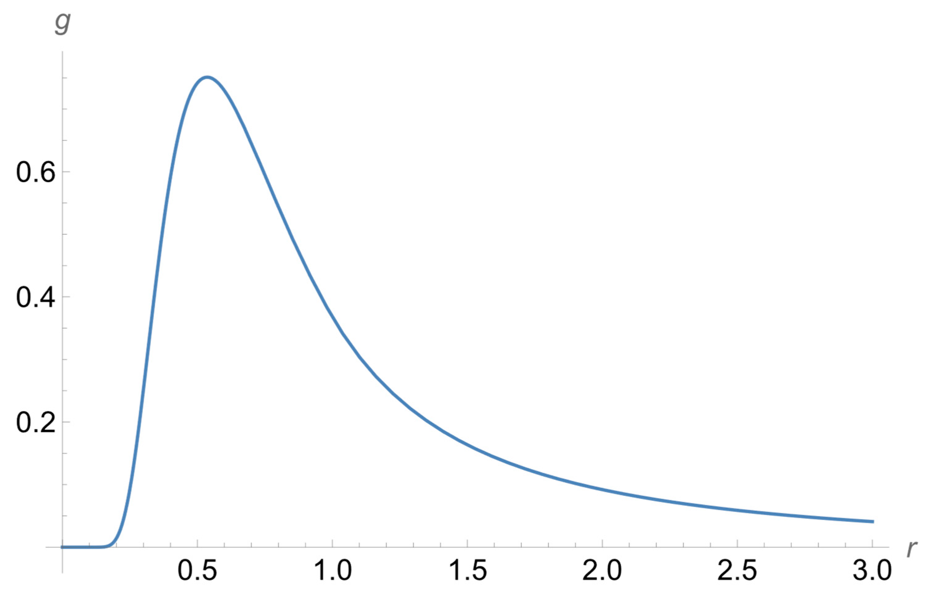
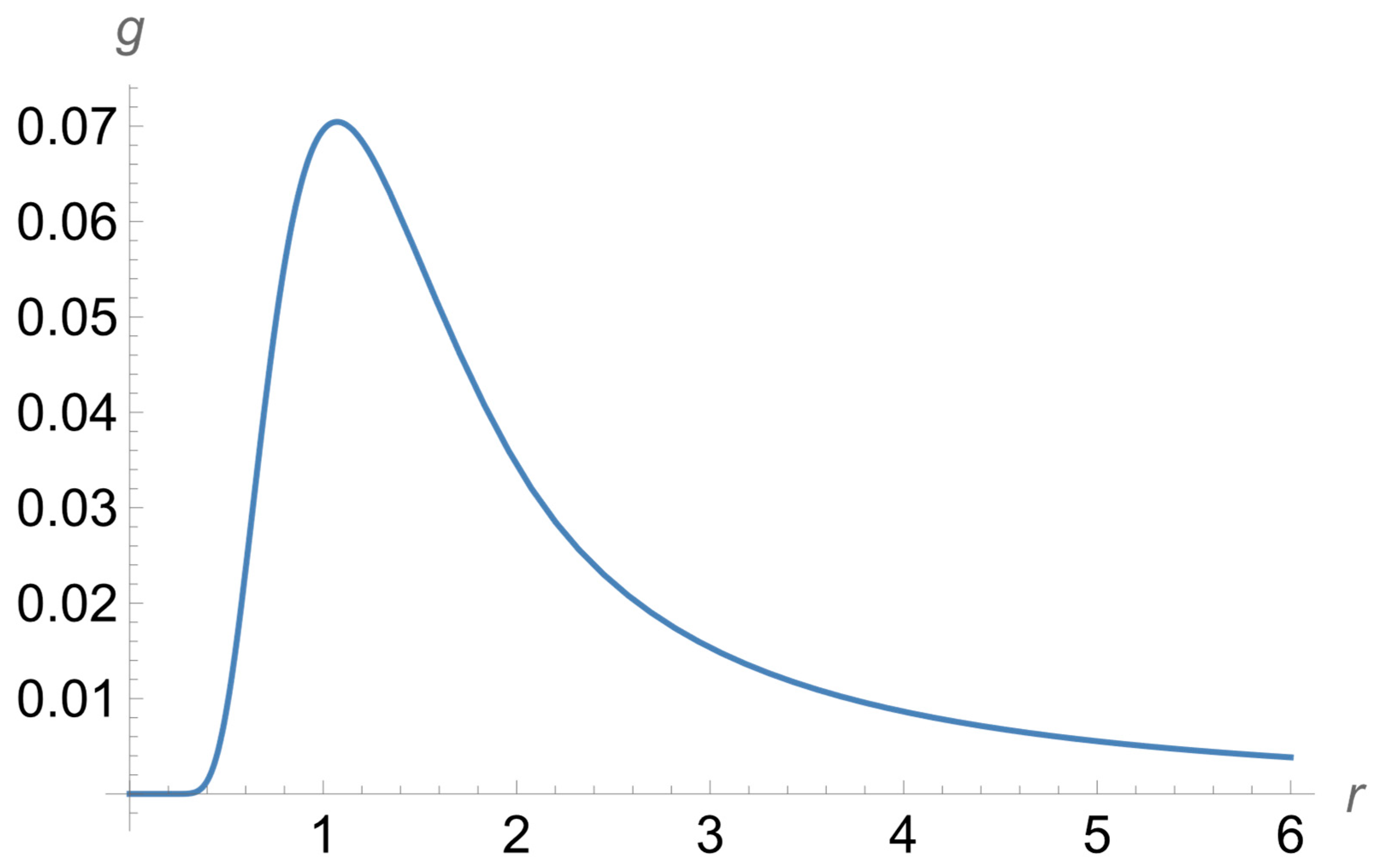
Figure 1 presents the dependence of the g-component of the wave function on r as we set R = 1 in some arbitrary unit of length. It is seen that the interior and exterior parts of the solution are perfectly matched at R = 1.
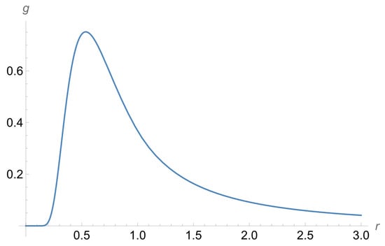
Figure 1.
Dependence of the g-component of the wave function on r as we set R = 1 in some arbitrary unit of length.
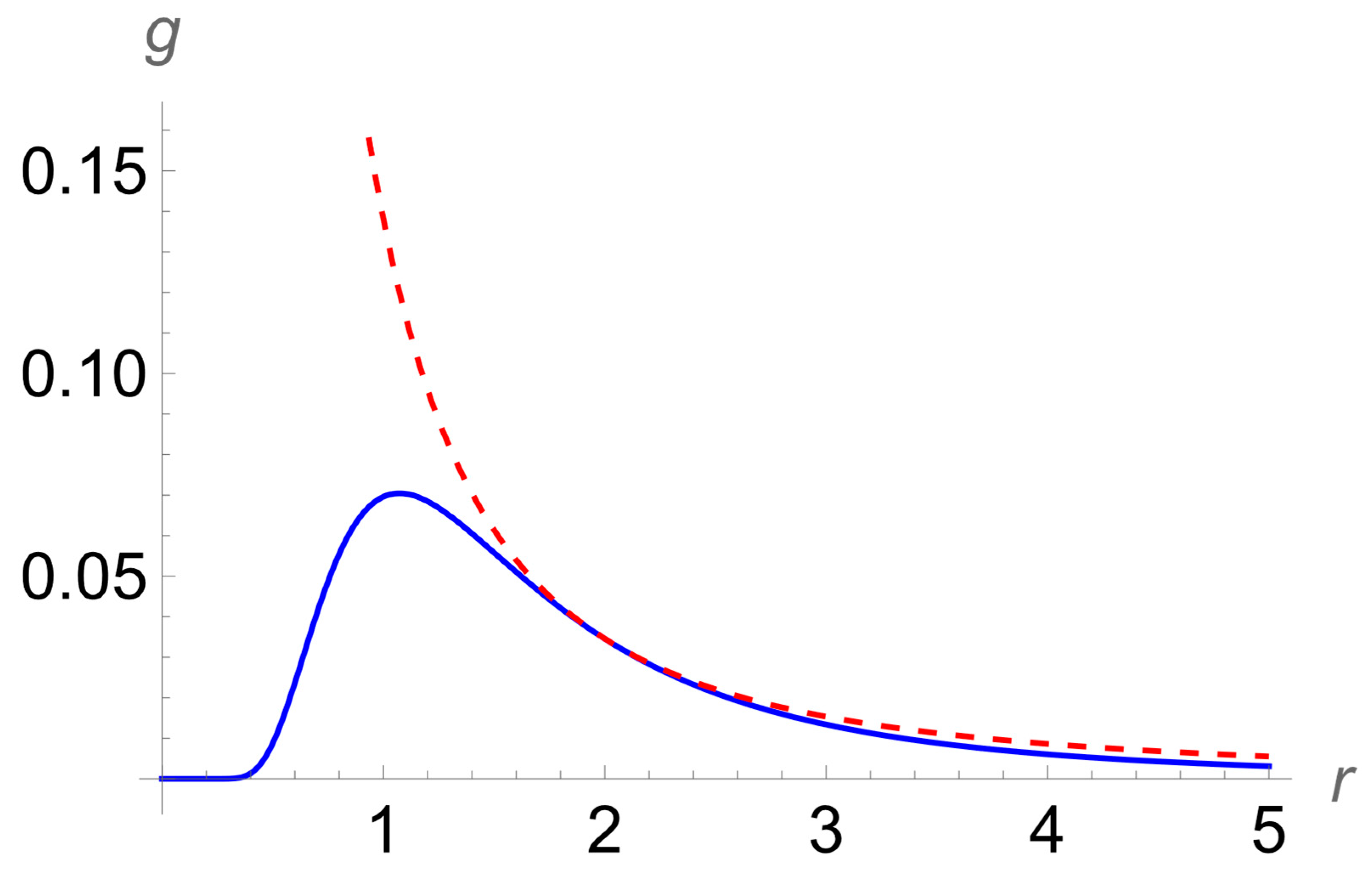
For illustrating the perfect match in more detail, we provide Figure 2 showing, by the solid line, gint(r) from Equation (35) and, by the dashed line, gext(r) from Equation (38). It is seen that at R = 1, there is a smooth transition from the solid line to the dashed line.
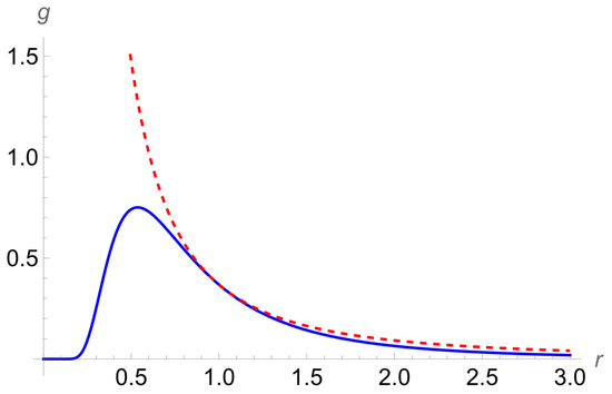
Figure 2.
The plots of gint(r) from Equation (35) (solid line) and of gext(r) from Equation (38) (dashed line) for R = 1.
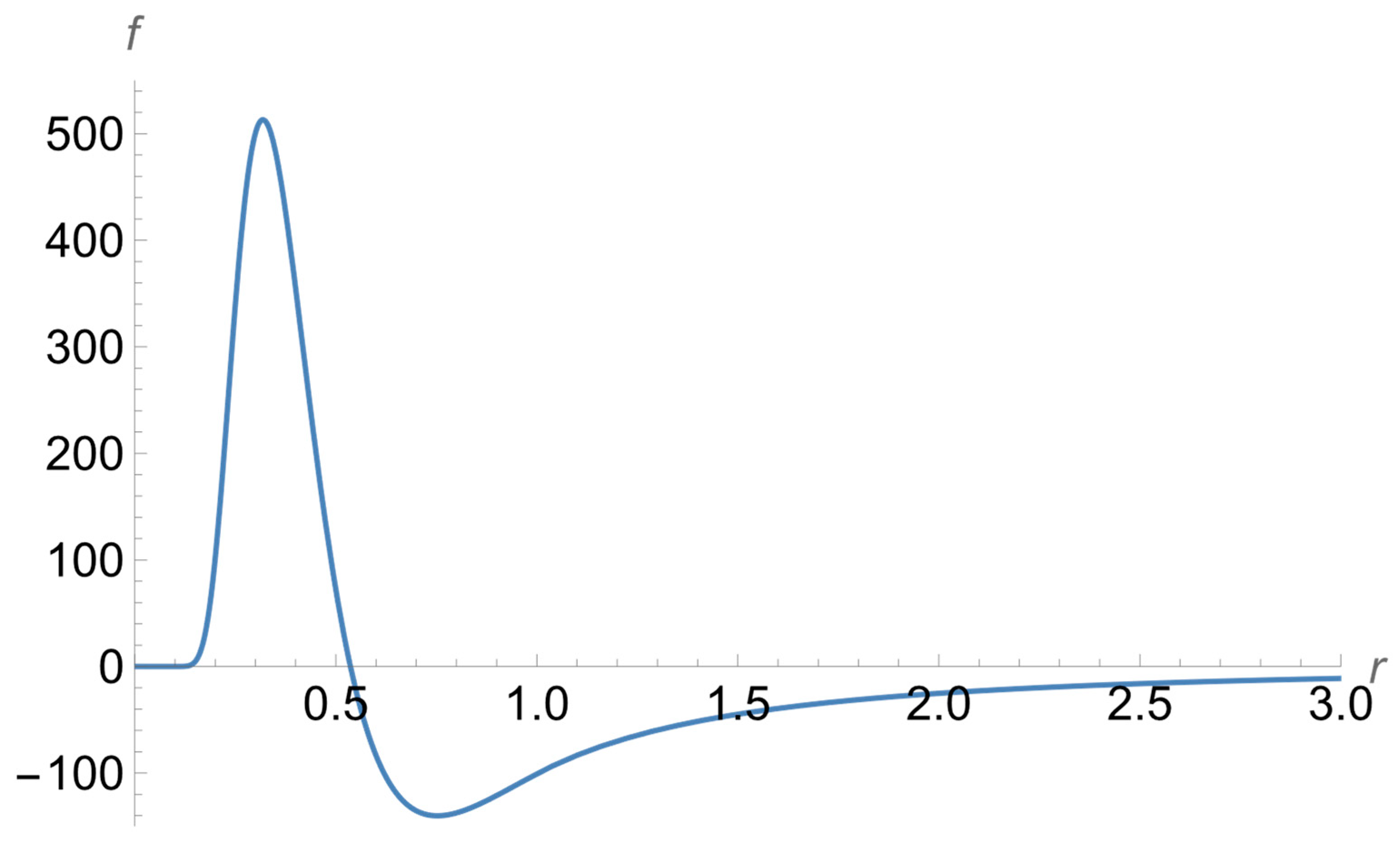
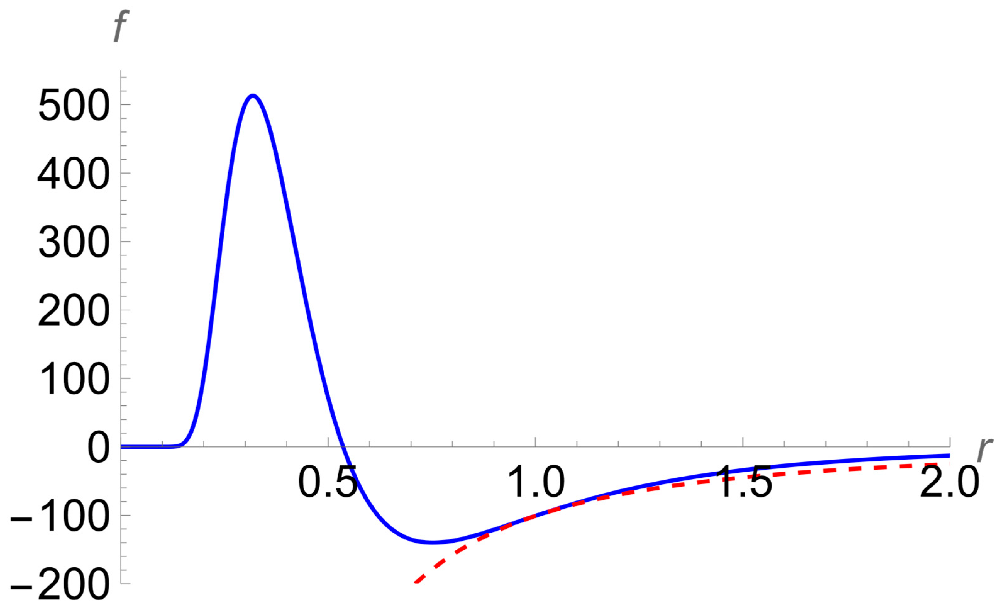
Figure 3 displays the dependence of the f-component of the wave function on r for R = 1. It is seen that the interior and exterior parts of the solution are perfectly matched at R = 1.
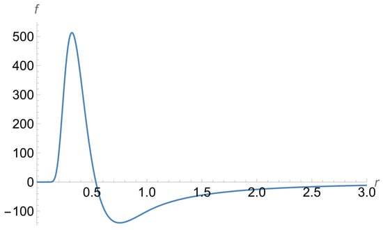
Figure 3.
Dependence of the f-component of the wave function on r for R = 1.
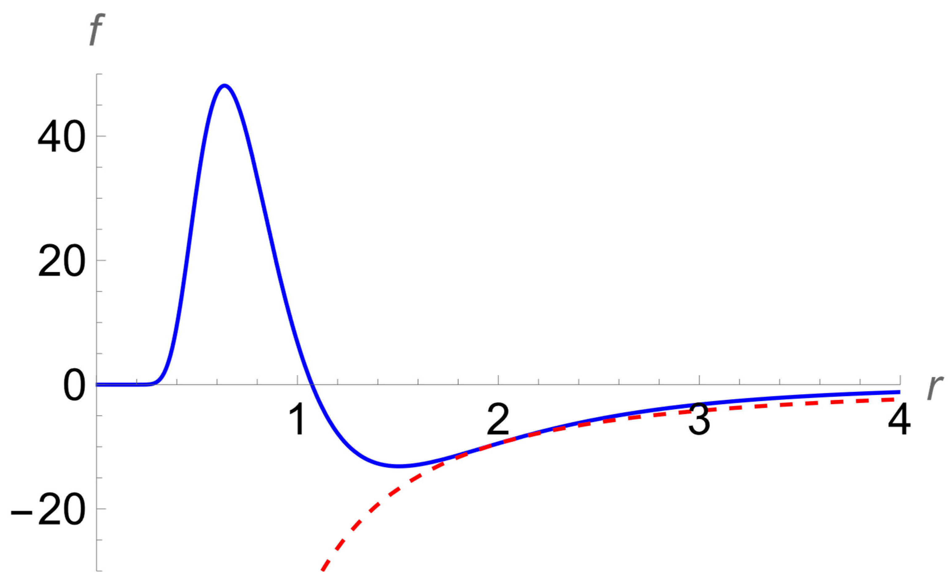
For illustrating the perfect match in more detail, we provide Figure 4 showing, by the solid line, fint(r) from Equation (36) and, by the dashed line, fext(r) from Equation (38). It is seen that at R = 1, there is a smooth transition from the solid line to the dashed line.
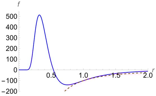
Figure 4.
The plots of fint(r) from Equation (36) (solid line) and of fext(r) from Equation (38) (dashed line) for R = 1.
Now, we demonstrate that the required match of the above interior and exterior solutions occurs regardless of the particular value of R. For this purpose, in Figure 5 we present the dependence of the g-component of the wave function for R = 2 in the same arbitrary unit of length as for R = 1. It is seen that the interior and exterior parts of the solution are perfectly matched at R = 2.
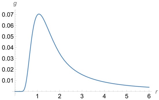
Figure 5.
Dependence of the g-component of the wave function for R = 2 in the same arbitrary unit of length, as for R = 1.
For illustrating the perfect match in more detail, we provide Figure 6 showing, by the solid line, gint(r) from Equation (35) and, by the dashed line, gext(r) from Equation (38). It is seen that at R = 2, there is a smooth transition from the solid line to the dashed line.
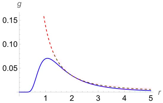
Figure 6.
The plots of gint(r) from Equation (35) (solid line) and of gext(r) from Equation (38) (dashed line) for R = 2.
Figure 7 displays the dependence of the f-component of the wave function on r for R = 2. It is seen that the interior and exterior parts of the solution are perfectly matched at R = 2.
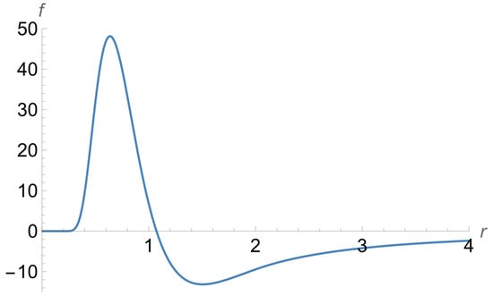
Figure 7.
Dependence of the f-component of the wave function on r for R = 2.
For illustrating the perfect match in more detail, we provide Figure 8 showing, by the solid line, fint(r) from Equation (36) and, by the dashed line, fext(r) from Equation (38). It is seen that at R = 2, there is a smooth transition from the solid line to the dashed line.
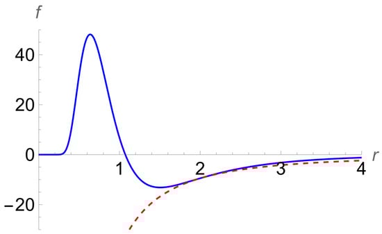
Figure 8.
The plots of fint(r) from Equation (36) (solid line) and of fext(r) from Equation (38) (dashed line) for R = 2.
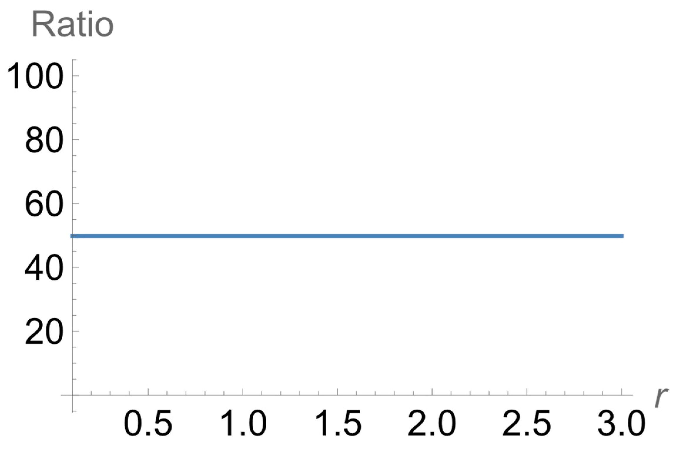
We found the following relation:
In words, the ratio g(R, Rr)/g(1,r) does not depend on r for any R. Figure 9 illustrates this fact for the example of R = π (the value R = π is chosen for demonstrating that the above statement is not limited to integer values of R).
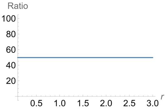
Figure 9.
The ratio g(R, Rr)/g(1,r) versus r for R = π.
Thus, the above interior and exterior solutions are scale-invariant with respect to the change of the boundary R between them. This invariance is the manifestation of the new symmetry of the Dirac equation.
The above completes the detailed theoretical proof of the existence of the SFHA. The rest of the paper concerns applications and has no bearing on the above theoretical proof of the existence of the SFHA. For completeness, we note that solutions of the Dirac equations were discussed not only in textbook [29] but in several other textbooks, such as, e.g., [37,38,39,40,41,42].
4. More Accurate Calculations Related to the Resolution of the Neutron Lifetime Puzzle
In the present paper, we provide more accurate calculations and details (on the neutron lifetime) that were not given in our paper [15], which was devoted primarily to neutron stars. (There was a misprint in the expression for gint(r) in Equation (3) from paper [15]: in the denominator, instead of r it should have been r2. This misprint was “inherited” from paper [3], where in the expression for gint(r) in Equation (17), the power of r in the denominator should have been increased by 1. In the above papers, the subsequent calculations were performed using the correct formulas, so that these misprints did not affect the results). First, the wave function, combining the results from Equations (35), (36), and (38) was complemented by the exponentially declining tail—the tail being similar to the regular solution of the corresponding Dirac equation (see, e.g., textbook [29]):
gtail(r) ~ 2 exp( −αr), ftail(r) ~ α exp(−αr).
Then, we calculated the normalization integral N(R):
In Equation (41), g2(R, r) and f2(R, r) are the wave functions of the second solution of the Dirac equation (based on Equations (35), (36), (38), and (40)), as indicated by the subscript “2”.
According to Bahcall [17], the probability P(R) of the 2-body decay of neutrons is proportional to the square absolute value of the wave function of the atomic electron at the proton surface, i.e., at r = R. So, we calculated the following Enhancement Factor (EF)
where
EF(R) = P2(R)/P1(R) = [g2N(R, R)2 + f2N(R, R)2]/[g1(R)2 + f1(R)2],
g2N(R, R) = g2(R, R)/[N(R)]1/2, f2N(R, R) = f2(R, R)/[N(R)]1/2.
In Equation (43), g1(R) and f1(R) are the well-known regular solutions of the Dirac equation for hydrogen atoms (see, e.g., textbook [29]).
On substituting in Equation (42) as the proton boundary R the experimental root-mean-square value of the proton radius 0.85 fm = 0.0022 n.u., we obtain EF~3 × 10³ >> 1. This means that the 2-body decay of neutrons should indeed lead to producing mostly the SFHA. The physical reason is that the rise of the wave functions in the direction of the proton (from the exterior) is much more robust for the second solution compared to the first solution.
The corresponding theoretical BR for the 2-body decay of neutrons becomes ~1%, which is indeed in very good agreement with the BR of (1.15 ± 0.27)% required for reconciling the experimental values of τtrap and τbeam. The neutron lifetime puzzle (sometimes called “anomaly”) seems to be likely resolved.
Finally, we note that the experimental verification of the above results could use as the starting point for the designs from papers [43] or [44], with modifications based on the properties of the SFHA. Details will be published elsewhere.
5. Conclusions
We obtained the explicit form of the solution of the Dirac equation inside the proton for the S-states—the solution that at the proton boundary matches the corresponding singular solution, as required by quantum mechanics, i.e., both the wave function and its derivative are continuous at the boundary. We demonstrated that such a solution inside the proton can be (and is) obtained within the class of functions that are non-analytic at r = 0—in distinction to the conventional practice of limiting the search for the solution by the class of analytic functions, i.e., by functions that can be adequately represented by their expansion into the Laurent series.
We showed that the interior and exterior solutions are scale-invariant with respect to the change of the boundary R between these two regions. Such invariance is the manifestation of a new symmetry—in addition to the previously discussed symmetries of the Dirac equation in the literature.
We used the obtained results for more accurate calculations related to the 2-body decay of neutrons and their application to resolving the neutron lifetime puzzle. On the basis of the more accurate calculations, we reconfirmed that the 2-body decay of neutrons produces mostly the SFHA and that the significantly increased BR for the 2-body decay becomes indeed sufficient for explaining the difference between the neutron lifetime values measured in the trap and beam experiments. Thus, our new, more accurate results for the wave function inside and outside the proton heightened the reliability of this resolution of the neutron lifetime puzzle.
Our results seem to be important both from the theoretical and experimental viewpoints. For example, they have profound cosmological consequences. They lead to viewing neutron stars in a new light as the generators of the baryonic DM in the Universe, as presented in paper [15].
Funding
This research received no external funding.
Data Availability Statement
All data are included in the paper.
Conflicts of Interest
The author declares no conflicts of interest.
Appendix A. The Experimental Charge Density Distribution Inside the Proton
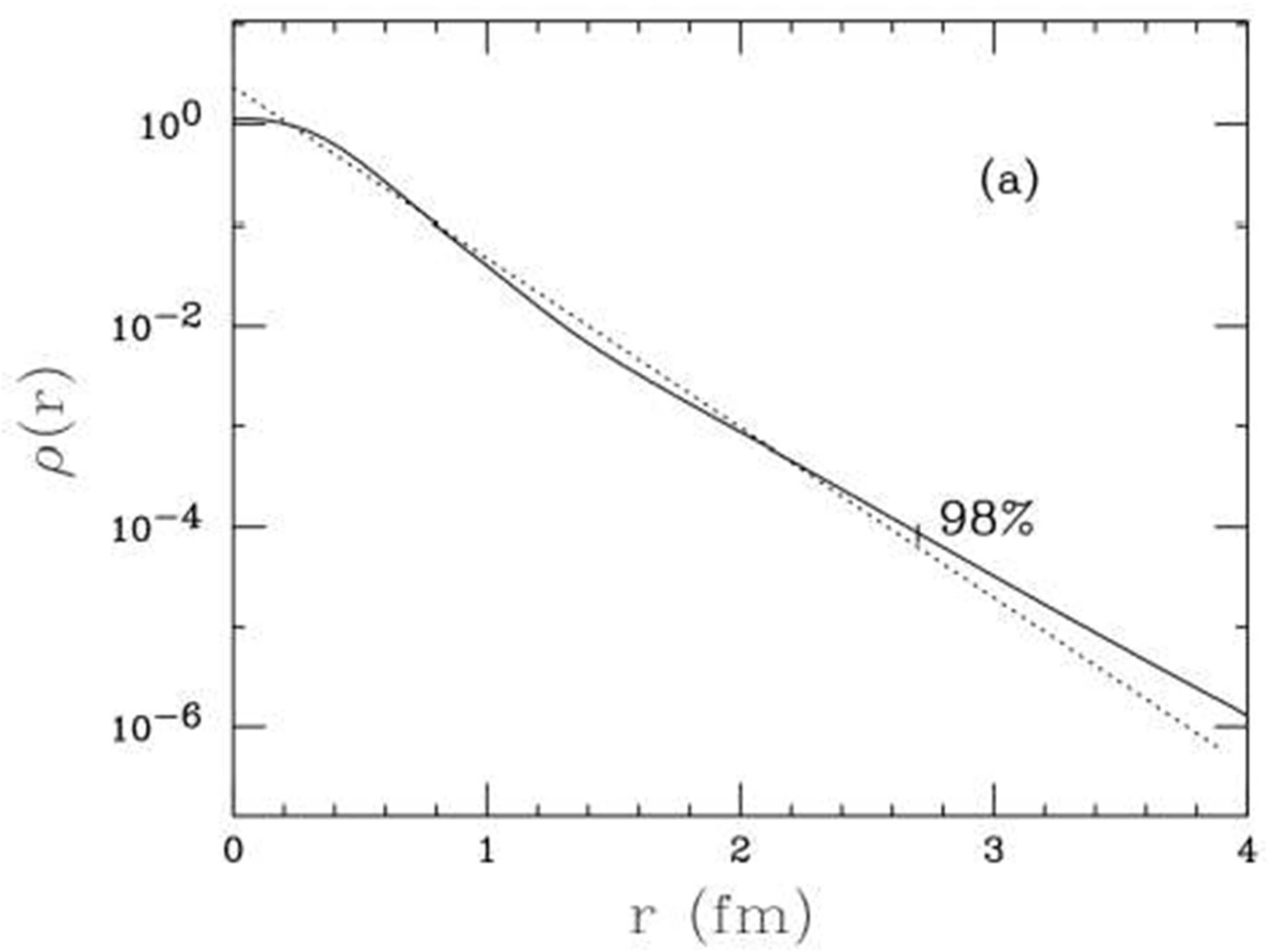
The most recent Charge Density Distribution (CDD) inside protons ρ(r), deduced from the corresponding experimental electric form-factors Ge(q), was presented in 2018 by Sick [45]—see Figure A1.

Figure A1.
The experimental charge density distribution inside the protons according to Sick [41]: the distribution corresponding to the dipole form factor (dotted line) and a more realistic one (solid line) resulting from the fit to the experimental electron scattering data. The mark 98% shows that integrating from 0 to 2.7 fm yields 98% of the rms-radius of protons.
The experimental Ge(q) values were taken from a variety of world data. In the non-relativistic limit, ρ(r) is related to Ge(q) via the Fourier transform:
The proton form factor is roughly described by the dipole shape:
where RD is the corresponding rms proton charge radius. The CDD corresponding to this form factor has the shape of an exponential:
GD(q) = 1/(1 + q2RD2/12)2,
ρD(r) ∝ exp(−121/2r/RD).
It is seen that the experimental CDD in protons (solid line) has the maximum at r = 0 and then monotonically falls-off to the periphery. This kind of CDD yields the potential satisfying, as a particular case, the general condition from Equation (14) from paper [3], under which the wave functions inside the proton can be matched at the proton boundary with the wave function of the singular solution outside the proton.
The commonly used characteristic parameter of any distribution (or of a spectral line shape) is its Half Width at Half Maximum (HWHM). For the experimental CDD shown by the solid line in Figure A1, we found HWHM ≈ 0.32 fm ≈ 0.00089 n.u.
References
- Gryzinski, M. Classical theory of atomic collisions. I. Theory of inelastic collisions. Phys. Rev. 1965, 138, A336. [Google Scholar]
- Fock, V. Zur Theorie des Wasserstoffatoms. Z. Phys. 1935, 98, 145. [Google Scholar] [CrossRef]
- Oks, E. High-energy tail of the linear momentum distribution in the ground state of hydrogen atoms or hydrogen-like ions. J. Phys. B At. Mol. Opt. Phys. 2001, 34, 2235. [Google Scholar]
- Oks, E. Alternative kind of hydrogen atoms as a possible explanation for the latest puzzling observation of the 21 cm radio line from the early Universe. Res. Astron. Astrophys. 2020, 20, 109. [Google Scholar] [CrossRef]
- Oks, E. Two Flavors of Hydrogen Atoms: A Possible Explanation of Dark Matter. Atoms 2020, 8, 33. [Google Scholar] [CrossRef]
- Wrkich, J.; Mathews, D.; Kanik, I.; Trajmar, S.; Khakoo, M.A. Differential Cross-Sections for the Electron Impact Excitation of the B 1Σu+, c 3Πu, a 3Σ+, C 1Πu, E, F 1Σ+ and e 3Σu+ States of Molecular Hydrogen. J. Phys. B At. Mol. Opt. Phys. 2002, 35, 4695–4709. [Google Scholar] [CrossRef]
- Mason, N.J.; Newell, W.R. The Total Excitation Cross Section of the c 3Πu State of H2. J. Phys. B At. Mol. Opt. Phys. 1986, 19, L587–L591. [Google Scholar]
- Ajello, J.M.; Shemansky, D.E. Electron Excitation of the H2(a 3Σg+ − b 3Σu+) Continuum in the Vacuum Ultraviolet. Astrophys. J. 1993, 407, 820–825. [Google Scholar] [CrossRef]
- Zammit, M.C.; Savage, J.S.; Fursa, D.V.; Bray, I. Electron-Impact Excitation of Molecular Hydrogen. Phys. Rev. A 2017, 95, 022708. [Google Scholar] [CrossRef]
- Oks, E. Experiments on the electron impact excitation of hydrogen molecules indicate the presence of the second flavor of hydrogen atoms. Foundations 2022, 2, 697–703. [Google Scholar] [CrossRef]
- Callaway, J.; McDowell, M.R.C. What we do and not know about electron impact excitation of atomic hydrogen. Comments At. Mol. Phys. 1983, 13, 19. [Google Scholar]
- Kauypila, W.E.; Ott, W.R.; Fite, W.L. Excitation of Atomic Hydrogen to the Metastable 22S1/2 State by Electron Impact. Phys. Rev. A 1970, 1, 1099–1108. [Google Scholar] [CrossRef]
- Whelan, C.T.; McDowell, M.R.C.; Edmunds, P.W. Electron impact excitation of atomic hydrogen. J. Phys. B At. Mol. Phys. 1987, 20, 1587. [Google Scholar] [CrossRef]
- Oks, E. Experiments on the electron impact excitation of the 2s and 2p states of hydrogen atoms confirm the presence of their second flavor as the candidate for dark matter. Foundations 2022, 2, 541–546. [Google Scholar] [CrossRef]
- Oks, E. New results on the two-body decay of neutrons shed new light on neutron stars. N. Astron. 2024, 113, 102275. [Google Scholar] [CrossRef]
- Gonzalez, F.M.; Fries, E.M.; Cude-Woods, C.; Bailey, T.; Blatnik, M.; Broussard, L.J.; Callahan, N.B.; Choi, J.H.; Clayton, S.M.; Currie, S.A.; et al. Improved neutron lifetime measurement with UCN τ. Phys. Rev. Lett. 2021, 127, 162501. [Google Scholar] [CrossRef]
- Bahcall, J.N. Theory of bound-state beta decay. Phys. Rev. 1961, 124, 495. [Google Scholar] [CrossRef]
- Bowman, J.D.; Rogers, A.E.E.; Monsalve, R.A.; Mozdzen, T.J.; Mahesh, N. An absorption profile centred at 78 megahertz in the sky-averaged spectrum. Nature 2018, 555, 67–70. [Google Scholar] [CrossRef]
- Barkana, R. Possible interaction between baryons and dark-matter particles revealed by the first stars. Nature 2018, 555, 71–74. [Google Scholar] [CrossRef]
- McGaugh, S.S. Research Notes of the Amer. Astron. Soc. 2018, 2, 37. [Google Scholar]
- Oks, E. The second flavor of hydrogen atoms constitutes most of baryonic dark matter. Int. J. Mod. Phys. D 2025, 34, 2550008. [Google Scholar] [CrossRef]
- Oks, E. Second flavor of heavy ions. Nucl. Phys. A 2023, 1040, 122758. [Google Scholar] [CrossRef]
- Marsch, E.; Narita, Y. CPTM symmetry for the Dirac equation and its extended version based on the vector representation of the Lorentz group. Front. Phys. 2021, 9, 618392. [Google Scholar] [CrossRef]
- Breev, A.I.; Shapovalov, A.V. The Dirac equation in an external electromagnetic field: Symmetry algebra and exact integration. J. Phys. Conf. Ser. 2016, 670, 012015. [Google Scholar] [CrossRef]
- Simulik, V.M.; Krivsky, A.Y. Bosonic symmetries of the Dirac equation. Phys. Lett. A 2011, 375, 2479–2483. [Google Scholar] [CrossRef]
- Ke, H.W.; Li, Z.; Chen, J.L.; Ding, Y.B.; Li, X.Q. Symmetry of Dirac Equation and Corresponding Phenomenology. arXiv 2009, arXiv:0907.0051. [Google Scholar] [CrossRef]
- Shapovalov, A.V.; Shirokov, I.V. Noncommutative integration method for linear partial differential equations. functional algebras and dimensional reduction. Theoret. Math. Phys. 1996, 106, 3–15. [Google Scholar] [CrossRef]
- Shapovalov, A.V.; Shirokov, I.V. Noncommutative integration of linear differential equations. Theoret. Math. Phys. 1995, 104, 921–934. [Google Scholar] [CrossRef]
- Rose, M.E. Relativistic Electron Theory; Sections 28, 29, 39; Wiley: New York, NY, USA, 1961. [Google Scholar]
- Mohammadi, F. An extended Legendre wavelet method for solving differential equations with non analytic solutions. J. Math. Ext. 2014, 8, 55–74. [Google Scholar]
- Hosseini, S.G.; Mohammadi, F. A new operational matrix of derivative for Chebyshev wavelets and its applications in solving ordinary differential equations with non analytic solution. Appl. Math. Sci. 2011, 5, 2537–2548. [Google Scholar]
- Mohammadi, F.; Hosseini, M.M.; Mohyud-Din, S.T. Legendre wavelet Galerkin method for solving ordinary differential equations with non-analytic solution. Intern. J. Syst. Sci. 2011, 42, 579–585. [Google Scholar] [CrossRef]
- Byers, P.; Himonas, A. Nonanalytic solutions of the KdV equation. In Abstract and Applied Analysis; Hindawi Publishing Corporation: London, UK, 2004; Volume 6, pp. 453–460. [Google Scholar]
- Bronshtein, M.D. Differential equations that have nonanalytic solutions. Uspekhi Mat. Nauk 1975, 30, 227–228. [Google Scholar]
- Oleinik, O.A.; Radkevich, E.V. A certain class of linear differential equations that have nonanalytic solutions. Uspekhi Mat. Nauk 1973, 28, 191–192. [Google Scholar]
- Oleinik, O.A.; Radkevich, E.V. Systems of differential equations that have nonanalytic solutions. Uspekhi Mat. Nauk 1972, 27, 247–248. [Google Scholar]
- Rebhan, E. Theoretische Physik: Relativistische Quantenmechanik, Quantenfeldtheorie und Elementarteilchentheorie; Springer: Berlin, Germany, 2010. [Google Scholar]
- Greiner, W. Relativistic Quantum Mechanics; Springer: Berlin, Germany, 2000. [Google Scholar]
- Bethe, H.A.; Salpeter, E.E. Quantum Mechanics of One- and Two-Electron Atoms; Dover: Mineola, NY, USA, 2008. [Google Scholar]
- Berestetskii, V.B.; Lifshitz, E.M.; Pitaevskii, L.P. Relativistic Quantum Theory; Pergamon: Oxford, UK, 1971. [Google Scholar]
- Davydov, A.S. Quantum Mechanics; Pergamon: Oxford, UK, 1965. [Google Scholar]
- Rojansky, V. Introductory Quantum Mechanics; Prentice Hall: Englewood Cliffs, NJ, USA, 1938. [Google Scholar]
- McAndrew, J.; Paul, S.; Engels, R.; Fierlinger, P.; Gutsmiedl, E.; Schön, J.; Schott, W. Bound beta-decay of the free neutron: BoB. Phys. Procedia 2014, 51, 37–40. [Google Scholar] [CrossRef]
- Nico, J.S.; Dewey, M.S.; Gilliam, D.M.; Wietfeldt, F.E.; Fei, X.; Snow, W.M.; Greene, G.L.; Pauwels, J.; Eykens, R.; Lamberty, A.; et al. Measurement of the neutron lifetime by counting trapped protons in a cold neutron beam. Phys. Rev. C 2005, 71, 055502. [Google Scholar] [CrossRef]
- Sick, I. Proton charge radius from electron scattering. Atoms 2018, 6, 2. [Google Scholar]


Disclaimer/Publisher’s Note: The statements, opinions and data contained in all publications are solely those of the individual author(s) and contributor(s) and not of MDPI and/or the editor(s). MDPI and/or the editor(s) disclaim responsibility for any injury to people or property resulting from any ideas, methods, instructions or products referred to in the content. |
© 2025 by the author. Licensee MDPI, Basel, Switzerland. This article is an open access article distributed under the terms and conditions of the Creative Commons Attribution (CC BY) license (https://creativecommons.org/licenses/by/4.0/).