Research on the Damage Mechanism and Shear Strength Weakening Law of Rock Discontinuities Under Dynamic Load Disturbance

Abstract

Discontinuity damage and shear strength weakening under dynamic loading are important causes of engineering rock instability. To study the damage mechanism of rock discontinuities under dynamic loading and the law of shear strength weakening after disturbance, the dominant controlling factors of dynamic loading-induced discontinuity damage were analyzed using the discrete element method. The evolution characteristics and formation mechanism of discontinuity damage were revealed, and the shear strength weakening law of discontinuities under dynamic loading was quantitatively characterized and verified by laboratory tests. The results are as follows: (1) Due to the symmetry of the structural distribution and material properties, a 2D UDEC-Tri model containing a discontinuity specimen was established. The number of failure blocks and the crack development length were calculated using Fish scripting in UDEC. Based on the orthogonal design method, it was found that the dominant controlling factors of dynamic load-induced discontinuity damage are the dynamic load frequency, peak dynamic load, and cycle number. (2) In the rising stress stage, the discontinuity mainly accumulates energy, causing minor damage with slight shear crack development. In the falling stress stage, energy release increases the damage, leading to significant shear and tensile crack growth with a hysteresis effect. The cracks are symmetrically distributed on both sides of the discontinuity. (3) The greater the damage to the discontinuity caused by the dynamic load disturbance, the more obvious the shear strength weakening after the disturbance. By comprehensively considering the symmetry characteristics of the damage distribution and strength weakening law of the discontinuity, and based on mathematical analysis, the model of discontinuity shear strength weakening after dynamic load disturbance was established. The model considers three dominant controlling factors: the dynamic loading frequency, peak dynamic load, and cycle number. The research results reveal the damage mechanism of discontinuities under dynamic loading and obtain the shear strength weakening law, which provides a reference for the stability evaluation of engineering rock masses under dynamic loading.

1. Introduction

Jointed rock masses are highly susceptible to dynamic disturbance. It has a significant impact on the engineering safety of mining infrastructure and resource development. Dynamic disturbances such as blast impacts, ramming-induced abrupt loads, seismic waves, vehicle vibrations, and other low-magnitude construction-related dynamic actions can directly trigger discontinuity instability or shear strength weakening. The 2007 collapse accident at the Gaoyangzhai tunnel entrance in Hubei Province, China, was an example of such engineering hazards [1]. Therefore, it is necessary to study the damage of discontinuities and the shear strength weakening law under dynamic loading.

Existing research has extensively investigated dynamic load-induced damage in homogeneous rocks. Hong et al. [2] evaluated the damage process of sandstone under dynamic loading from the perspective of microscopic crack propagation through theoretical models and experiments and established a model for the propagation of wing cracks that effectively predicts the strength of sandstone. Liu et al. [3] revealed the damage and failure mechanism of granite during the loading and unloading process by counting tensile and shear cracks through discrete element software. Shi et al. [4] studied the macroscopic deformation characteristics of sandstone under dynamic loading by cyclic dynamic loading tests and revealed the relationship between energy evolution and dissipation characteristics and the deformation and damage law of sandstone. Geranmayeh Vaneghi et al. [5] found that rock specimens exhibited strength degradation under dynamic loading compared to static loading by carrying out uniaxial cyclic compression tests. Kim et al. [6] established an in situ rock damage evolution assessment method through incremental cyclic dynamic loading tests and numerical simulations, demonstrating the feasibility of using acoustic emission technology to quantitatively evaluate the evolution of rock damage under dynamic loading.

For rock masses containing discontinuities, the effects of dynamic loading show increased complexity. Niktabar et al. [7] studied the effect of different frequencies on joints through dynamic load shear tests and found that the frequency dominates the initial peak shear stress, revealing the law of change in the joint shear mechanism. Soomro et al. [8] established a calculation model for the critical shear strain of rock joints and a classification method for the sliding potential of rock joints through cyclic triaxial tests, revealing the influence of the number of cycles on the stability of rock joints. Peellage et al. [9,10] analyzed the relationship between the amplitude of the shear stress and the damage of joint over-deformation by performing dynamic cyclic tests on jointed rock samples and found that parameters such as the critical shear stress and elastic modulus under dynamic loading deteriorate significantly. Siamaki et al. [11] analyzed the damage and shear strength of discontinuities after repeated vibration loading through blast vibration records and particle flow numerical simulations, revealing the law of crack damage and shear strength degradation of discontinuities under dynamic loading. Gao et al. [12] used numerical experiments to study the effect of discontinuity vibration deterioration under the influence of different factors and derived and proposed a discontinuity vibration deterioration model. Zheng et al. [13] studied the shear strength and deformation characteristics of limestone through true triaxial multi-stage cyclic shear tests and acoustic emission monitoring, proposed a three-dimensional shear strength criterion that considers lateral stress, established a mechanical model that considers parameter degradation, and verified its effectiveness.

Most of the above studies on the influence of dynamic load disturbance on rock masses with discontinuities have focused on dynamic load disturbance during shearing. However, through the engineering statistical analysis of existing research [14], the instability of many projects occurred after a period of time when the dynamic load disturbance had ceased, i.e., the dynamic load disturbance caused discontinuity damage before the shear slip occurred. Therefore, it is necessary to study the damage mechanism of rock discontinuities under dynamic load disturbance and the shear strength weakening law after disturbance separately. In this paper, the discrete element method is used to analyze the dominant controlling factors of blast dynamic load-induced structural damage, to reveal the structural damage evolution characteristics and mechanisms, and to obtain the shear strength weakening law of the discontinuity under dynamic load disturbance, which is verified by laboratory tests.

2. Numerical Simulation Protocol for Dynamic Load Disturbance in Rock Discontinuity

2.1. Model Construction and Parameter Calibration

There are many methods that exist for numerical modeling [15,16,17]. Due to the consideration of the influence of dynamic loads on damage to rock discontinuities and to better observe the cracking and deformation characteristics of rock discontinuities during dynamic loading, a UDEC simulation specimen containing a discontinuity was created. The model was divided into several triangular blocks using a Voronoi trigon. Since each triangular block is an independent deformable body, the constitutive model of the block is set to the commonly used Mohr–Coulomb model. During the dynamic loading process, each microscopic block and contact will experience corresponding changes in force and displacement. The change in the joints near the discontinuity will be manifested as damage to the entire discontinuity on a macroscopic scale. Therefore, the joint and the discontinuity are set to an area Coulomb slip model to better reproduce the damage characteristics of rock discontinuities under dynamic loading. Figure 1a shows a schematic diagram of the numerical model with an inclination angle of 30° and JRC = 8–10. Here, it is assumed that the mechanical properties and structural distribution of the rock are the same in different cross-sections; that is, they are isotropic in different cross-sections, which belongs to the plane strain model. This behavior is essentially a manifestation of symmetry in material properties and structural distribution. On the same cross-section, the blocks and joints satisfy rotational symmetry along the discontinuity. At the same time, the distribution of each joint direction and each block is different, exhibiting anisotropy, which is consistent with the actual rock discontinuities.

The model is a two-dimensional rectangle with dimensions of 50 mm × 100 mm, which facilitates studying the influence of the inclination angle of the discontinuity. The maximum size of the triangular block is 4 mm. The y-direction velocity of the grid point node at the lower boundary is set to 0 to fix the direction, and the dynamic load is applied from the upper boundary downward. To make the results more intuitive, the maximum length of the longest edge of the triangles near the discontinuities is set to 2 mm for densification, and the material parameters of the blocks in this area are reduced accordingly. This is consistent with the fact that, in reality, a certain amount of rock debris on the discontinuities results in smaller rock parameters [18]. The reduction is determined based on factors such as the degree of rock weathering and the degree of fracture development and is generally assumed to be between 0.3 and 0.7 of the original value [19,20]. In this case, 0.3 is used. The macroscopic deformation of the block is determined by the two parameters of bulk modulus K and shear modulus G, while the macroscopic deformation of joints and discontinuity is determined by the two parameters of normal stiffness K_n and tangential stiffness K_s. The relationship between them is determined by Equations (1) and (2).

$$K={\displaystyle \frac{E}{3\left(1-2\nu \right)}},G={\displaystyle \frac{E}{2\left(1+\nu \right)}}$$

(1)

$$K_s=0.4K_n$$

(2)

where E is the modulus of elasticity of the block and ν is the Poisson ratio of the block. The relevant physical parameter values are shown in

Table 1. Block mechanical parameters.

	Density (kg/m3)	Bulk Modulus K (Pa)	Shear Modulus G (Pa)	Friction Angle $\mathit{\varphi }$ (°)	Cohesion C (Pa)	Tensile Strength T (Pa)
Blocks at both ends	2160	2.38 × 109	1.32 × 109	43	6.72 × 106	3.83 × 106
Blocks near discontinuity	2160	7.80 × 108	4.50 × 108	43	2.06 × 106	1.12 × 106

and

Table 2. Joint mechanical parameters.

	Normal Stiffness Kn (Pa/m)	Shear Stiffness Ks (Pa/m)	Friction Angle $\mathit{\phi }$ (°)	Cohesion c (Pa)	Tensile Strength t (Pa)
Joints at both ends	4.16 × 1013	1.66 × 1013	39	6.72 × 106	3.83 × 106
Joints near discontinuity	4.16 × 1013	1.66 × 1013	39	2.06 × 106	1.12 × 106
Discontinuity	4.16 × 1013	1.66 × 1013	39	0.0	0.0

. The parameters of the blocks and the joints at each end were determined by the trial-and-error method. They are similar in strength to the deeply buried mudstone of a particular mine [21]. A comparison of the stress–strain curves calibrated with the parameters is shown in Figure 1b. The specimen strength of the parameters set for the blocks and joints near the discontinuity is similar to the reduced uniaxial strength of the mudstone.

To ensure that the upper and lower disc blocks are always in contact with each other through discontinuity, an axial load of 1 MPa is first applied and maintained, and all subsequent dynamic loads are superimposed on it. The triangular waveform shown in Figure 1c is selected as the dynamic load waveform to simulate blast dynamic loads. Each triangle waveform is divided into two stages: a rising stress stage and a falling stress stage. The ratio of the rise time to the fall time is calculated according to Equation (3) and is always 1:10.

$$t_{end}=10t_{peak}$$

(3)

where t_peak is the time to peak stress and t_end is the total time of a single cycle.

2.2. Orthogonal Experimental Design for Dynamic Load Disturbance

In order to study the dominant controlling factors that lead to damage on the discontinuity under dynamic load disturbance, in combination with existing research [22,23,24], five influencing factors are considered: the peak dynamic load, dynamic loading frequency, cycle number, discontinuity inclination angle, and discontinuity roughness. Each influencing factor is considered at five levels. The dynamic loading frequency is taken as the frequency of blasting loads, which cause greater damage in engineering [25,26,27], and is set at a gradient of 100 Hz in the range of 100–500 Hz. The roughness coefficient was obtained by rotating the specified angles and reducing them proportionally according to Barton standard joint profile lines No. 3 (JRC = 4–6), No. 5 (JRC = 8–10), No. 8 (JRC = 14–16), and No. 10 (JRC = 18–20) [28,29]. The horizontal values of each influencing factor are shown in

Table 3. The level values of five influencing factors.

Levels	Factors
	Peak Dynamic Load (MPa)	Cycle Number (times)	Dynamic Loading Frequency (Hz)	Inclination Angle (°)	Roughness
1	5	1	100	0	0
2	7.5	2	200	10	5
3	10	3	300	20	9
4	12.5	4	400	30	15
5	15	5	500	40	19

, and roughness is expressed as the average value of the corresponding section.

The orthogonal design method is a method for studying multi-factor, multi-level problems. By selecting representative experimental points and arranging an orthogonal table, the effect of a large number of experiments can be obtained with only a small number of experiments [30,31,32]. The core of it is the symmetrical and even distribution of the experimental points; that is, the geometric symmetry is presented through the experimental combinations of the orthogonal table, which avoids local errors and thus determines the global law through some experiments. The five factors and five levels selected were arranged in an L25 (5⁵) orthogonal table according to the orthogonal design method, for a total of 25 groups. The specific design is shown in

Table 4. Orthogonal design schemes.

Group Number	Peak Dynamic Load (MPa)	Cycle Number (times)	Dynamic Loading Frequency (Hz)	Inclination Angle (°)	Roughness	Group Number	Peak Dynamic Load (MPa)	Cycle Number (times)	Dynamic Loading Frequency (Hz)	Inclination Angle (°)	Roughness
1	15.0	2	100	20	5	14	15.0	1	400	30	9
2	5.0	4	200	20	9	15	7.5	2	500	10	9
3	10.0	5	300	0	9	16	5.0	1	100	0	0
4	5.0	3	500	30	15	17	10.0	2	200	30	0
5	12.5	4	300	30	5	18	15.0	3	300	10	0
6	7.5	4	400	40	0	19	10.0	4	100	10	15
7	7.5	1	300	20	15	20	12.5	5	500	20	0
8	10.0	3	400	20	19	21	12.5	1	200	10	19
9	15.0	4	500	0	19	22	10.0	1	500	40	5
10	7.5	5	100	30	19	23	5.0	2	300	40	19
11	12.5	2	400	0	15	24	12.5	3	100	40	9
12	5.0	5	400	10	5	25	15.0	5	200	40	15
13	7.5	3	200	0	5

.

3. Dominant Controlling Factors and Formation Mechanisms of Discontinuity Damage Under Dynamic Load Disturbance

3.1. Characterization Indices for Discontinuity Damage

To study the evolution process of discontinuity damage under dynamic loading, the Fish language function built into the UDEC 7.0 software was used for programming. The number of failure blocks, the crack propagation length, and dissipated energy during the loading process were counted. Changes in the first two parameters can directly reflect the degree of damage to the rock discontinuities, while the dissipated energy can reflect the energy dissipation during dynamic loading. The number of failure blocks is the sum of the number of blocks that fail in tension and the number of blocks that fail in shear, calculated using Equation (4). The crack propagation length is the sum of the propagation lengths of tensile cracks and shear cracks, calculated using Equation (5). Dissipated energy is the difference between the loading work and the total strain energy, calculated using Equation (6).

$$N_b=N_{bs}+N_{bt}$$

(4)

$$L_j=L_{js}+L_{jt}$$

(5)

$$W_j=W-U_c$$

(6)

Among them, N_b is the number of failure blocks. N_bs and N_bt are the number of blocks that have experienced shear failure and tensile failure, respectively. L_j is the crack propagation length. L_js and L_jt are the propagation lengths of shear cracks and tensile cracks, respectively. W_j is the total dissipated energy in joints. W and U_c are the work done and the total strain energy of the material, respectively.

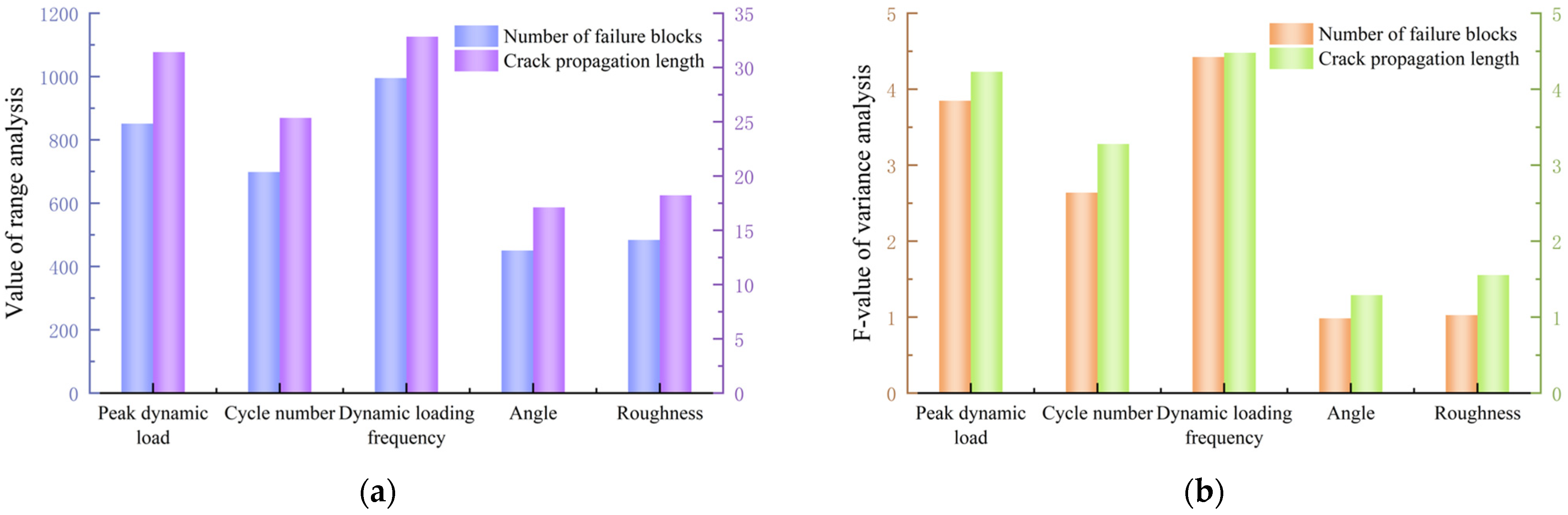
3.2. Sensitivity Analysis for Different Influencing Factors

Table 5. Damage index values of each group.

Group Number	Number of Failure Blocks (Number)	Crack Propagation Length (cm)	Group Number	Number of Failure Blocks (Number)	Crack Propagation Length (cm)
1	58	3.74	14	373	3.03
2	72	2.96	15	162	5.13
3	119	7.40	16	2	0.49
4	416	8.37	17	70	9.30
5	179	7.03	18	97	11.03
6	218	12.14	19	93	4.13
7	1	0.17	20	1941	69.51
8	18	1.12	21	137	3.62
9	2508	93.06	22	260	7.61
10	130	4.61	23	32	0.91
11	113	8.89	24	341	9.29
12	4	0.63	25	1733	59.58
13	2	0.24

shows the specific data obtained from numerical simulations using the discrete element method for the two indicators, the number of failure blocks, and the crack propagation length, which facilitates range analysis and analysis of variance.

A range analysis is a method of measuring the degree of data dispersion by calculating the difference between the maximum and minimum values in a set of data. The range is the difference between the maximum and minimum mean values for each level of a single factor. The greater the range, the greater the influence of the factor on the indicator, and vice versa [30,31,32]. The average values for each factor and level for the two indicators of the number of failure blocks and crack propagation length were calculated, and the range of each factor is shown in

Table 6. The average value and range of the number of failure blocks.

Levels	Factors
	Peak Dynamic Load (MPa)	Cycle Number (Times)	Dynamic Loading Frequency (Hz)	Inclination Angle (°)	Roughness
1	105	155	125	549	466
2	103	87	403	99	81
3	112	175	62	418	213
4	633	723	145	247	471
5	954	785	1057	517	565
Range	851	698	995	450	484

and

Table 7. Average and range of crack propagation length.

Levels	Factors
	Peak Dynamic Load (MPa)	Cycle Number (Times)	Dynamic Loading Frequency (Hz)	Inclination Angle (°)	Roughness
1	2.67	2.98	4.45	22.02	20.49
2	4.46	5.60	15.14	4.91	2.44
3	5.91	6.01	3.90	15.50	5.56
4	18.26	22.46	5.16	5.06	16.23
5	34.09	28.35	36.74	17.90	20.66
Range	31.42	25.36	32.83	17.11	18.22

. Figure 2a shows the histogram of the range of each factor for the two damage indices. The dynamic loading frequency, peak dynamic load, and cycle number are ranked in the top three, with the range of each exceeding that of the roughness or inclination angle by more than 30%. This result shows that the dynamic loading frequency, peak dynamic load, and cycle number have a greater impact on discontinuity under dynamic loading in the range analysis.

The analysis of variance can test for significant differences in the means of two or more samples. When dealing with multi-factor differences within and between groups, the F-test is performed using the mean square error ratio of each factor to determine whether a single factor has a significant effect [30,31,32]. The data in Table 5 were imported into SPSS 27.0 software for the analysis of variance, and the results of the main effect test are shown in

Table 8. Variance analysis of numbers of block failures.

Source	Type III Sum of Squares	Degrees of Freedom	Mean Square	F-Value	Significance	Ranking
Corrected model	9,709,510.800	20	485,475.54	2.584	0.185
Intercept	3,297,129.64	1	3,297,129.6	17.549	0.014
Peak dynamic load	2,892,135.76	4	723,033.94	3.848	0.110	2
Cycle number	1,982,242.16	4	495,560.54	2.638	0.185	3
Dynamic loading frequency	3,324,510.56	4	831,127.64	4.424	0.089	1
Inclination angle	739,263.36	4	184,815.84	0.984	0.506	5
Roughness	771,358.96	4	192,839.74	1.026	0.490	4
Error	751,546.56	4	187,886.64
Total	137,58187	25
Corrected total	10,461,057.36	24

and

Table 9. Variance analysis of crack propagation length.

Source	Type III Sum of Squares	Degrees of Freedom	Mean Square	F-Value	Significance	Ranking
Corrected model	12,595.178	20	629.759	2.966	0.150
Intercept	4461.52	1	4461.52	21.011	0.010
Peak dynamic load	3591.85	4	897.963	4.229	0.096	2
Cycle number	2784.24	4	696.06	3.278	0.138	3
Dynamic loading frequency	3805.01	4	951.253	4.48	0.088	1
Inclination angle	1095.43	4	273.858	1.29	0.406	5
Roughness	1318.65	4	329.661	1.553	0.340	4
Error	849.353	4	212.338
Total	17906.1	25
Corrected total	13444.5	24

. Figure 2b shows the analysis of the variance F-value histogram for the two damage indices of each factor. The F-values of dynamic loading frequency, peak dynamic load, and cycle number also ranked in the top three in order, all more than twice the F-value of the roughness or inclination angle. It can be seen that the dynamic loading frequency, dynamic loading peak value, and cycle number are dominant controlling factors on the damage to the discontinuity under dynamic loading in the analysis of variance.

Data were obtained by designing orthogonal experiments and performing numerical simulations. A sensitivity analysis of the two damage indices was carried out using range analysis and analysis of variance. It was concluded that the dynamic loading frequency, peak dynamic load, and cycle number are the dominant controlling factors affecting the damage to discontinuities under dynamic loading.

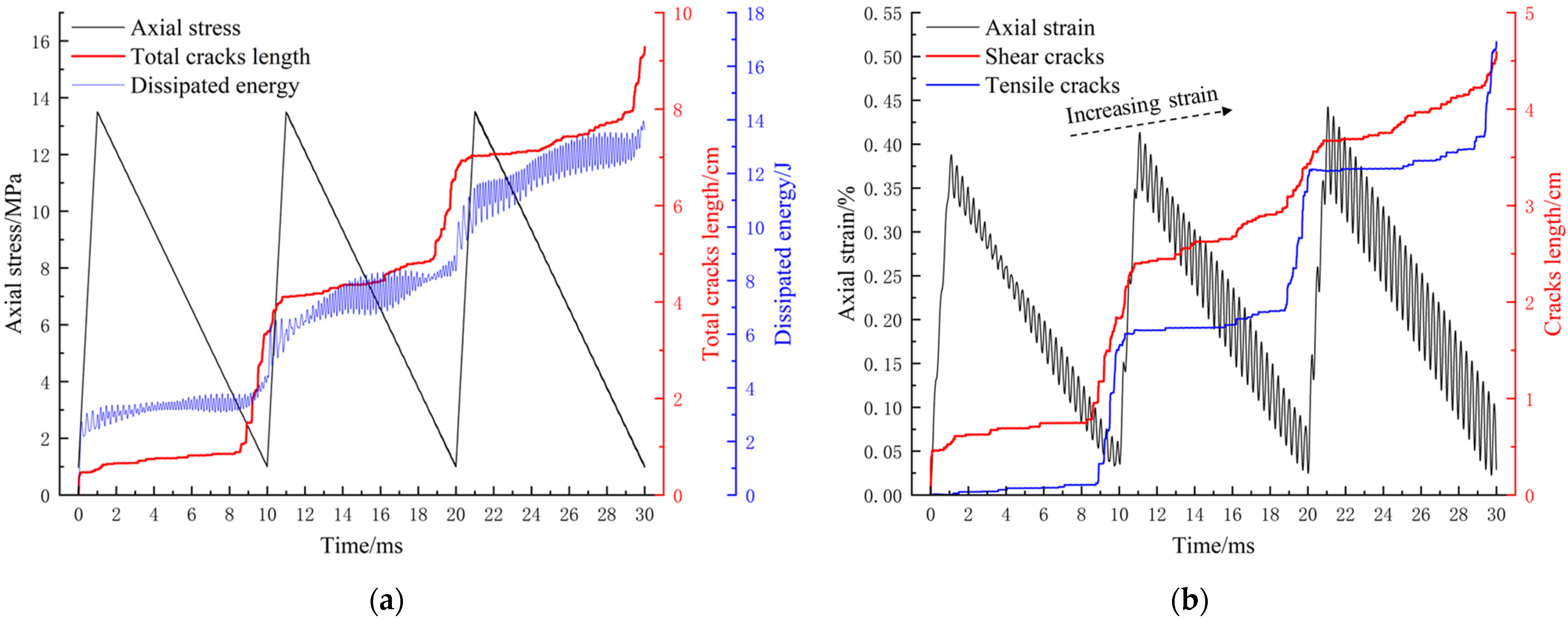
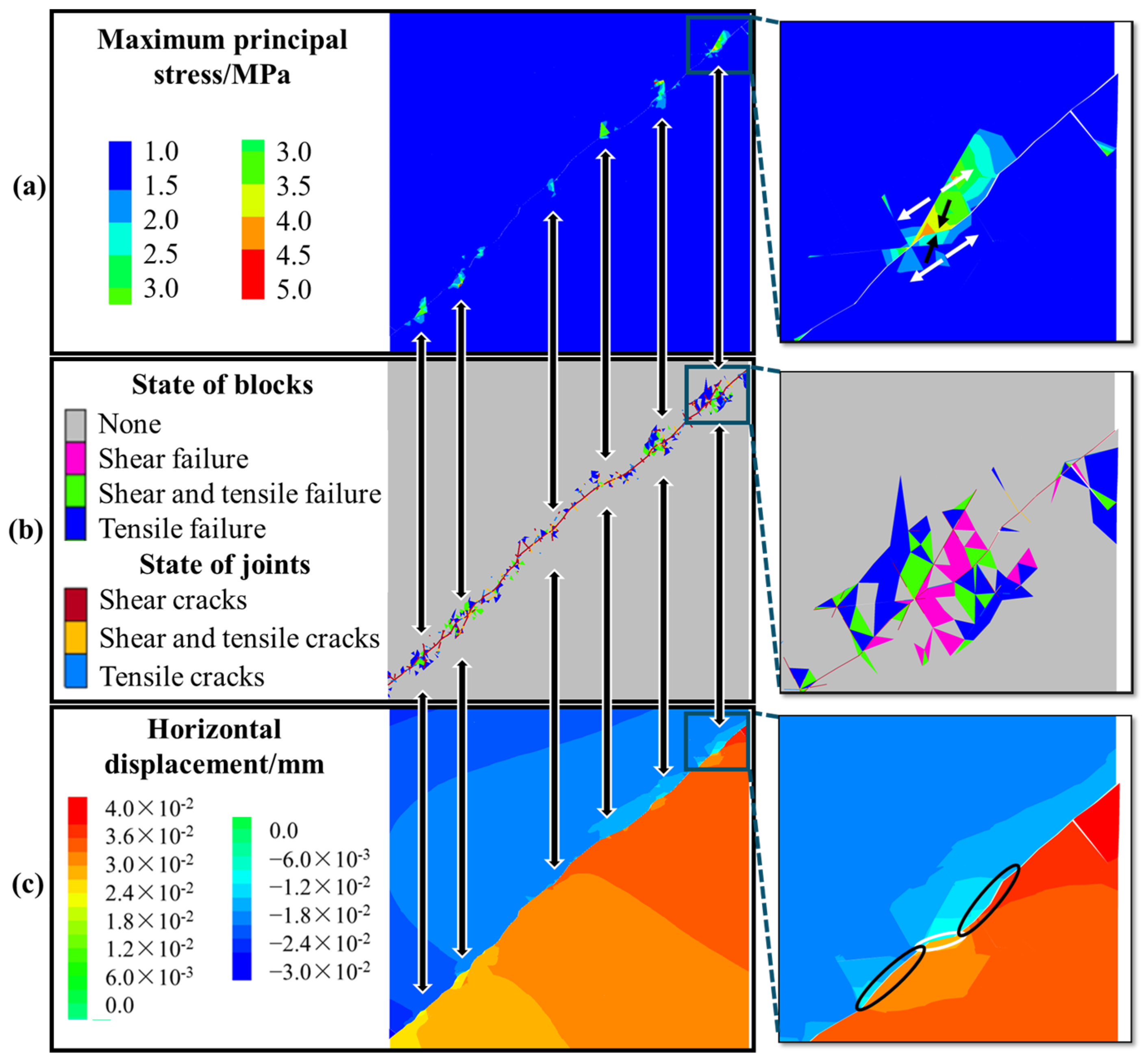
3.3. Characteristics and Formation Mechanism of Discontinuity Damage

Figure 3a shows the relationship between the axial stress of the specimen, crack propagation length, and dissipated energy over time during the application of a dynamic load. Figure 3b shows the relationship between the axial strain, tensile cracks, and shear crack propagation length over time. The peak dynamic load was 12.5 MPa, the cycle number was 3, the dynamic loading frequency was 100 Hz, the inclination angle was 40°, and the roughness JRC = 8–10.

As can be seen from Figure 3, during the rising stress stage, the stress on the joints increases at the beginning of loading, the strain rises steadily, and friction and slippage occur on the discontinuities, resulting in a small instantaneous increase in dissipated energy and the instantaneous development of shear cracks. Thereafter, the stress gradually reaches equilibrium, some of the joints begin to stretch, tensile cracks develop slowly, and crack development is inhibited by the increase in stress, with energy gradually accumulating. Both shear and tensile cracks develop insignificantly.

Then, it enters the falling stress stage. During the initial unloading period, the direction of dynamic load unloading gradually undergoes rebound deformation, strain oscillation decreases, the stress inhibition effect weakens, and the joints tend to develop, resulting in oscillating changes in dissipated energy and a slow increase. The development of both shear and tensile cracks is small. After a period of energy accumulation and an increase in rebound deformation, dissipated energy begins to increase significantly, and micro-cracks develop significantly. Shear cracks begin to develop significantly before tensile cracks because shear failure is more likely to occur near discontinuity.

Due to the susceptibility to shear damage in the vicinity of the discontinuity, shear cracks begin to develop much earlier than tensile cracks. In contrast, tensile cracks must overcome the tensile strength of the joints between the blocks. When the dissipated energy reaches a certain threshold, the development of tensile cracks shows more significant mutations and develops faster than that of shear cracks. The development of shear cracks mainly occurs at the end of the rising stress stage and falling stress stage, when the shear force between joints can reach the threshold of shear crack development. The development of tensile cracks mainly occurs at the end of the falling stress stage, when the tensile force between joints can reach the threshold of tensile crack development.

Crack development and joint energy dissipation show similar patterns for each cycle. Damage to discontinuities occurs primarily in the later stages of the cycle, lagging behind the increase in dynamic stress and exhibiting a damage hysteresis effect. Due to the incremental strain and damage accumulation caused by the cumulative fatigue damage effects of multiple cycles, more joints reach the damage threshold in the later cycles than in the earlier ones, and the time at which the level of damage increases substantially gradually approaches the time of peak dynamic load stress, and the damage hysteresis effect is mitigated. If the dynamic loading frequency increases and the time of a single cycle decreases, the damage hysteresis phenomenon may become more pronounced.

Figure 4 shows the distribution of damage areas on the simulated specimen under dynamic loading. The morphology of the cracks can be clearly seen macroscopically. The block failure and cracks are mainly concentrated in the area near the discontinuity, and the distribution position is significantly related to the morphology and trend in the discontinuity. The areas with large undulations of discontinuity have more severe damage to the blocks and joints; the areas with a gentle trend have slightly less damage. The shear failure of the blocks and the shear cracks in the joints are usually distributed closely along the discontinuity. This is because the blocks on both sides of the discontinuity are under compression, and shear damage occurs as they slip along the direction of the discontinuity. Tensile damage usually occurs around shear damage because the sheared area and the adjacent area do not move in the same direction along the slip direction, causing tension between the blocks and resulting in tensile failure.

Figure 5 presents the principal stress distribution, damage patterns, and localized displacements in the primary damage zone. Under dynamic loading, misalignment occurs between the rough discontinuity surfaces during upper/lower disc sliding, creating non-contact cavities (black zones in Figure 5c inset) that experience reduced stress concentrations and predominantly tensile damage. Conversely, contacting regions (white zones in Figure 5c inset) undergo shear damage due to non-parallel alignment between axial compressive stresses (black arrows in Figure 5a inset) and discontinuity orientation, inducing slippage. The contact periphery exhibits sharp stress and displacement gradient boundaries, with stress concentrations (white arrow in Figure 5a inset) arising from uneven displacement and stress distributions causing structural damage.

Multiple cyclic disturbances induce axial compression–rebound behavior, generating oscillatory displacement at contact points that accelerates progressive damage accumulation. Increasing dynamic load peaks amplifies stress and deformation gradients, intensifying damage in concentration zones. Macroscopically, symmetrical damage distribution manifests at both discontinuity ends, as evidenced in Figure 5b, showing matching bilateral damage patterns, demonstrating equivalent dynamic loading effects across the discontinuity. Microscopically, reverse symmetry emerges in damage propagation and horizontal displacements. As can be seen in Figure 5b,c, under the action of the force, the damage develops, and the horizontal displacement of the upper and lower blocks tends to develop in opposite directions.

4. Law of Shear Strength Weakening of Discontinuity After Dynamic Load Disturbance

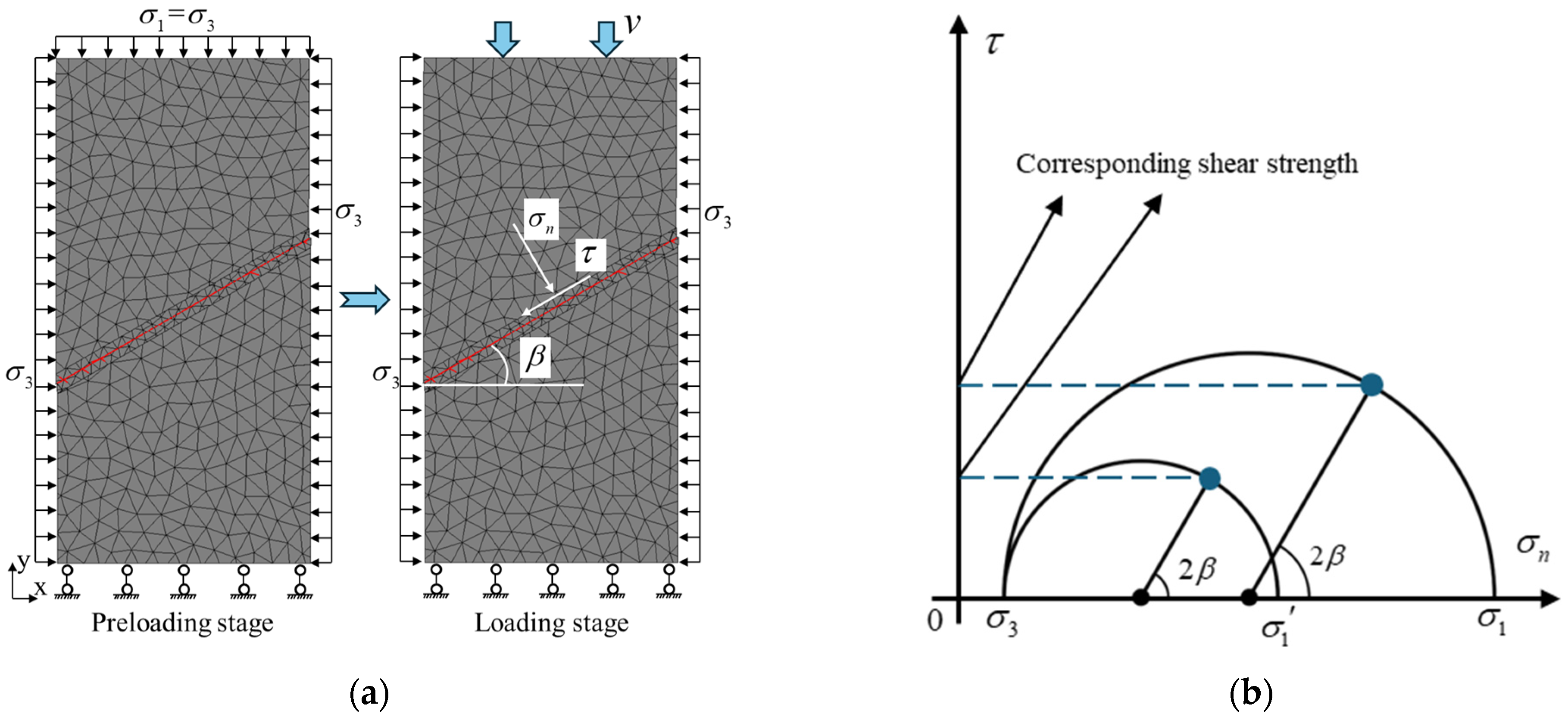
4.1. Calculation Method for the Shear Strength of Discontinuities After Dynamic Load Disturbance

In order to further study the shear strength change rule of rock discontinuities after being disturbed by dynamic loads, simulated triaxial tests were carried out on the simulated specimens after disturbance to determine their strength changes according to the existing research [33,34].

Figure 6 shows the main steps and calculation principles for obtaining the discontinuity shear strength on the simulated specimen after disturbance. In the first step, the y-direction of the lower boundary node is fixed, and 1 MPa confining pressure is applied to the left, right, and upper boundaries for a period of time. In the second step, the stress on the upper boundary is released, and a velocity constraint is applied in the negative y-direction until the simulated specimen fails. The stress and strain curves of the triaxial process are obtained by monitoring the force at the lower boundary node. The confining pressure of 1 MPa is used because the simulated specimen has been subjected to dynamic load disturbance, and it is not suitable for applying a larger confining pressure, so 1 MPa is selected with reference to existing studies [35].

The triaxial compressive damage of rocks containing discontinuities follows the Mohr–Coulomb strength theory, and the shear strength of the discontinuity can be obtained by triaxial testing [36,37,38,39]. The shear and normal stresses on the discontinuity during loading are expressed in Equations (7) and (8).

$${\sigma }_n={\displaystyle \frac{{\sigma }_1+{\sigma }_3}{2}}+{\displaystyle \frac{{\sigma }_1-{\sigma }_3}{2}}\cos \left(2\beta \right)$$

(7)

$$\tau ={\displaystyle \frac{{\sigma }_1-{\sigma }_3}{2}}\sin \left(2\beta \right)$$

(8)

When the boundary stress and the angle of inclination are fixed, i.e., ${\sigma }_3$ and $\beta$ are constant, the shear strength of the discontinuity can be calculated from the maximum peak principal stress ${\sigma }_{1,max}$ during triaxial loading, where the shear stress on the corresponding Mohr circle is the discontinuity shear strength.

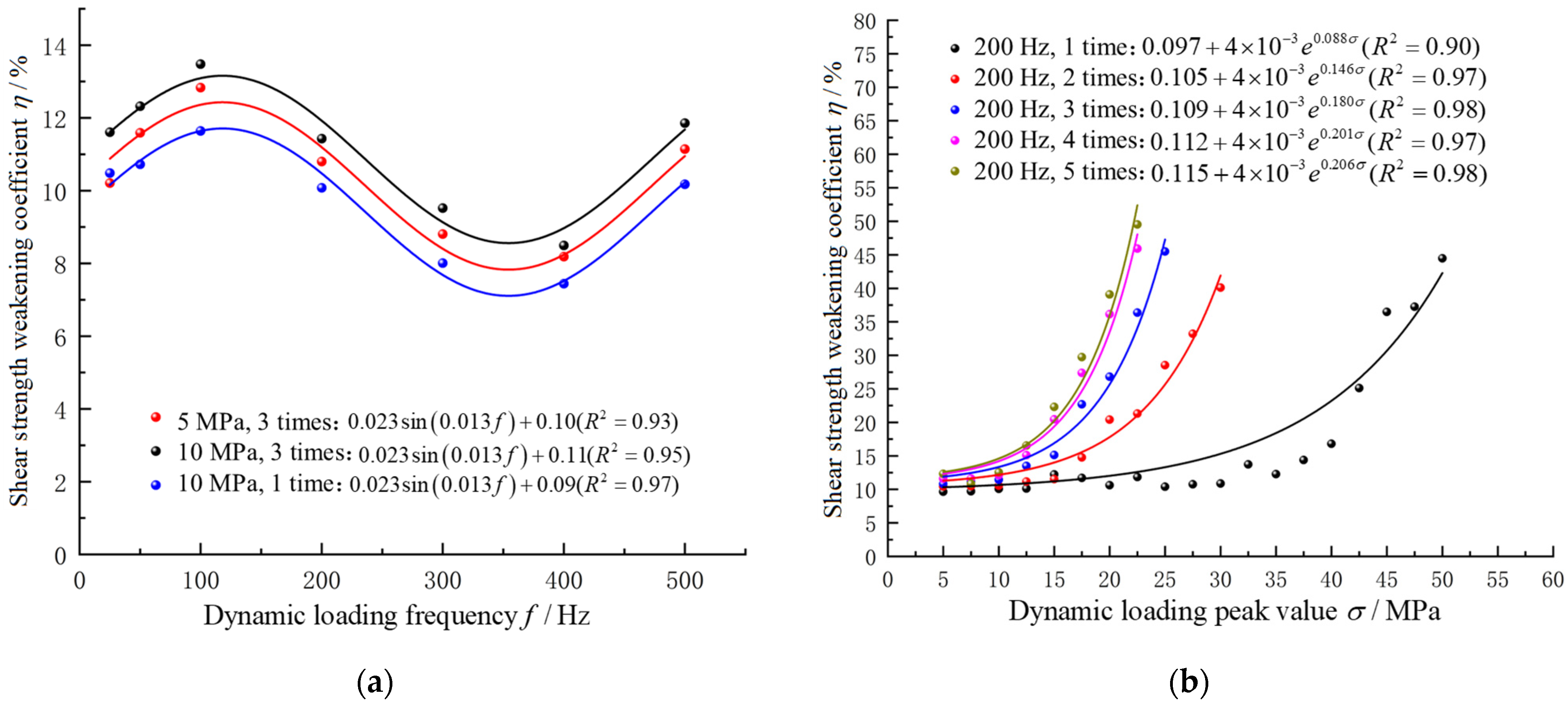
4.2. The Weakening Law of the Shear Strength of the Discontinuity Under the Dominant Controlling Factors

According to the results of the sensitivity analysis of different factors, the shear strength weakening model of discontinuity mainly considers three factors: the dynamic loading frequency, peak dynamic load, and cycle number. The inclination angle of the discontinuity is always kept constant at 30°, and JRC = 0. To obtain a more obvious strength weakening law, it is necessary to appropriately extend the value range of the dominant controlling factors on the basis of the orthogonal design scheme. The dynamic loading frequency is supplemented with 50 and 25 Hz, and the peak dynamic load is continuously increased by a gradient of 2.5 MPa until a significant law is obtained.

Figure 7 demonstrates the effect of different peak values on the stress–strain curve of the discontinuous surface under dynamic loading (200 Hz, three cycles). It is shown that the maximum principal stress peak ${\sigma }_{1,max}$ can effectively characterize the change rule of the discontinuity surface shear strength. Compared with the static load, the dynamic disturbance significantly reduces the shear strength of the discontinuous surface, and the strength decay is positively correlated with the degree of damage. When the peak value of the dynamic load increases, the damage of the specimen intensifies, resulting in obvious curve fluctuations and a consequent decrease in the elastic modulus. It is worth noting that even a small dynamic load disturbance can cause the upper and lower discs to slip due to the inclination angle of the discontinuity, resulting in a significant decrease in the shear strength, which indicates that the dynamic disturbance not only directly causes damage to the structure but also continuously affects the strength of the discontinuity through the weakening effect.

Knowing the confining pressure ${\sigma }_3$ and the inclination angle $\beta$, ${\sigma }_1$ is substituted into Equation (8) to calculate the shear strength, and the ratio of the difference between the shear strength before and after the dynamic load disturbance and the shear strength not perturbed by the dynamic load is defined as the shear strength weakening coefficient of the discontinuity, which is calculated as shown in Equation (9).

$$\eta ={\displaystyle \frac{{\tau }_s-{\tau }_d}{{\tau }_s}}=1-{\displaystyle \frac{{\tau }_d}{{\tau }_s}}={\displaystyle \frac{{\sigma }_{1,s}-{\sigma }_{1,d}}{{\sigma }_{1,s}-{\sigma }_3}}$$

(9)

where ${\tau }_d$ and ${\tau }_s$ are the shear strength of the discontinuity after being perturbed by dynamic loads and after being undisturbed. ${\sigma }_{1,s}$ and ${\sigma }_{1,d}$ are the peak maximum principal stresses in the three axes after being perturbed by dynamic loads and after being undisturbed, respectively.

Figure 8a shows the scatter plot of the shear strength weakening coefficient as a function of the dynamic loading frequency and its fitted curve. According to the simulation results in Figure 8a, the law of the weakening coefficient changing with the frequency is the same when other factors are changed. It is assumed that the frequency of the dynamic load, the peak dynamic load, and the cycle number affect each other independently. The influence of the dynamic loading frequency on the rock discontinuities is often related to its resonant frequency, which in turn is affected by many factors and changes. The interaction between the two can cause fluctuations in the strength of the rock discontinuities [40]. Therefore, a trigonometric function is used for fitting. Its regularity is expressed in periodicity and symmetry. Then, the shear strength weakening coefficient $\eta$ can be expressed as Equations (10) and (11).

$$\eta \left(f,\sigma ,n\right)=F\left(f\right)\cdot F\left(\sigma ,n\right)$$

(10)

$$F\left(f\right)=A_1\sin \left(B_{1}f\right)+C_1$$

(11)

It can be assumed that $F\left(f\right)$ exists as a coefficient in Equation (10), and the values of the parameters in Equation (11) can be calibrated by normalizing and then fitting the scatter data of Figure 8a.

Next, the relational equation of $F(\sigma ,n)$ is examined. Figure 8b shows the scatter and its fitting curve for the variation in the shear strength weakening coefficient with the peak dynamic load for different cycle numbers; at the same cycle number, the weakening coefficient first increases slowly as the peak dynamic load increases and then increases significantly after reaching a certain peak dynamic load. Thus, $F(\sigma ,n)$ can be described in terms of an exponential function, as shown in Equation (12).

$$F\left(\sigma ,n\right)=A_2+B_2{e}^{C_2\sigma }$$

(12)

The influence curve of A₂ in Equation (13) moves up and down in the horizontal coordinate, B₂ determines the initial value and the range of variation in the influence curve, and C₂ determines the growth rate of the curve. Combined with the curve in Figure 8b, the parameters A₂ and C₂ are greatly affected by the cycle number n, so they can be regarded as functions related to the cycle number n. Equation (12) can then be expressed as Equation (13).

$$F\left(\sigma ,n\right)=A_2\left(n\right)+B_2{e}^{C_2\left(n\right)\sigma }$$

(13)

As shown in Figure 8b, under the same peak dynamic load, the weakening factor increases with the increase in cycle number, and the growth range gradually decreases. Therefore, the changing relationship between A₂(n) and C₂(n) in Equation (13) with respect to n can be expressed as Equation (14).

$$\left\{\begin{array}{l}{A}_2\left(n\right)=a_1\ln n+a_2\\ C_2\left(n\right)=b_1\ln n+b_2\end{array}\right.$$

(14)

In Equation (14), a and b can be determined by fitting the curve. At this point, a model for the shear strength weakening of discontinuities under the dominant controlling factors can be obtained; that is, Equation (10) is expressed in Equation (15), which includes only the dynamic loading frequency, the peak dynamic load, and the cycle number.

$$\eta \left(f,\sigma ,n\right)=\left(A_1\sin \left(B_{1}f\right)+C_1\right)\cdot \left[a_1\ln n+a_2+B_2{e}^{\left(b_1\ln n+b_2\right)\sigma }\right]$$

(15)

By putting together the numbers from the numerical simulation in this paper, the values of each parameter in Equation (15) are found to make a model for how discontinuities weaken shear strength when certain factors are dominant. Equation (16) illustrates this result.

$$\eta \left(f,\sigma ,n\right)=\left(0.21\sin \left(0.013f\right)+0.95\right)\cdot \left[\left(0.011\ln n+0.097\right)+0.004e^{\left(0.076\ln n+0.091\right)\sigma }\right]$$

(16)

Two shear strength indicators that can be used directly in engineering are the cohesion and internal friction angle. Therefore, it is necessary to convert the shear strength of the discontinuity after weakening due to dynamic load disturbance into these two shear strength indicators. According to the Mohr–Coulomb strength criterion, the discontinuity shear strength weakening model can be applied to Equation (17), and then the two shear strength indicators can also be expressed by Equation (18), which gives the shear strength indicator of the discontinuity after dynamic load disturbance.

$$\left\{\begin{array}{l}{\tau }_d=\eta \left(f,\sigma ,n\right){\tau }_0\\ {\tau }_0={\sigma }_n\tan \left({\phi }_0\right)+c_0\end{array}\right.$$

(17)

$$\left\{\begin{array}{l}\tan \left({\phi }_d\right)=\eta \left(f,\sigma ,n\right)\tan \left({\phi }_0\right)\\ c_d=\eta \left(f,\sigma ,n\right)c_0\end{array}\right.$$

(18)

In fact, the discontinuity shear strength weakening model obtained in this paper is a modification of the discontinuity strength index after dynamic load disturbance. The modified parameters can also be used in existing models. For example, the Barton model takes into account the roughness of discontinuities more, but not the dynamic load disturbance. This model is helpful to predict the shear strength of discontinuities after being disturbed by dynamic loads during engineering construction and take targeted measures to avoid causing engineering rock mass instability.

5. Laboratory Test Verification of the Damage Mechanism and the Law of Strength Weakening

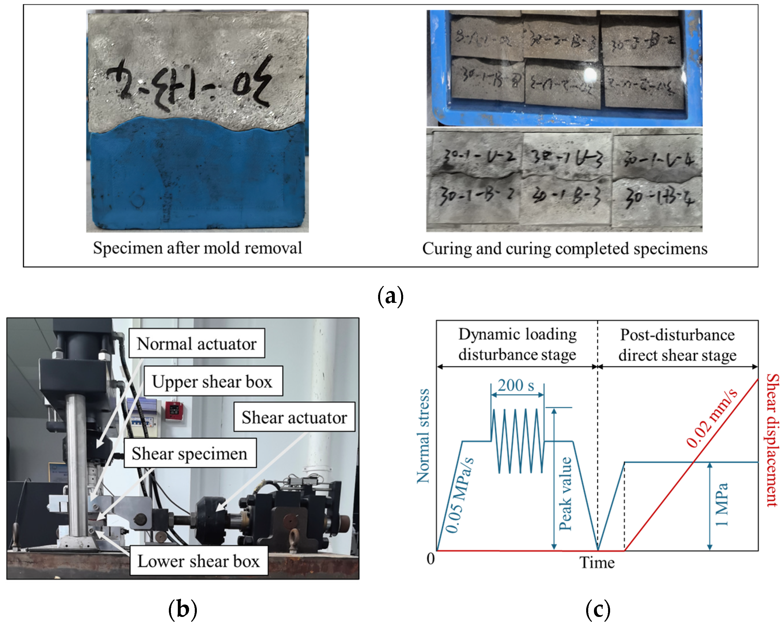
5.1. Laboratory Test Verification Plan

Numerous studies have shown that rock-like materials poured with cement, sand, and other raw materials have mechanical properties similar to actual engineered rock masses [41]. In this laboratory test, a specimen poured with a mixture of cement, quartz sand, and water at a ratio of 5:10:2 was used. Since the verification test solely takes into account the dominant controlling factors, we can use the direct shear test to determine the shear strength of the discontinuity. The specimen size is 100 × 100 × 100 mm³. The upper and lower specimens are cast separately using 3D printing molds. The discontinuity takes on a three-dimensional shape composed of the Barton standard curve. The three-dimensional shape of each group of specimens is exactly the same, as shown in Figure 9a. The uniaxial compressive strength of the concrete cubes from the same batch was measured to be about 27 MPa, and Young’s modulus was about 4.16 × 10⁹. The compressive strength of the engineering mudstone specimen calibrated by numerical simulation is 29.1 MPa, and the elastic modulus is about 4.02 × 10⁹. The parameters of the two are similar, and the error is within 10%.

The test uses the GCTS-RDS-200XL rock direct shear system to apply dynamic loads and perform direct shear after disturbance, as shown in Figure 9b. Figure 9c shows the laboratory test procedure, which consists of two stages: (1) The dynamic load disturbance stage: The shear displacement is always kept at 0. First, a normal load is applied at a speed of 0.05 MPa/s to the target value and maintained; then, a dynamic load is applied in the normal direction. The dynamic load adopts a triangular waveform with a fixed dynamic loading frequency and duration, with the peak dynamic load as a factor. Finally, following the application of the dynamic load, the load unloads at a rate of 0. (2) Direct shear stage after disturbance: First, a normal servo load of 1 MPa is applied at a normal loading rate of 0.05 MPa/s, followed by direct shear at a rate of 0.02 mm/s after holding pressure. The shear displacement is set to 10 mm and finally unloaded to obtain the shear strength of the post-fault discontinuity. In the laboratory, verification tests are performed to verify the laws of numerical simulation. For the specific plans, see

Table 10. Laboratory test verification plans.

Group Number	Peak Dynamic Load (MPa)	Dynamic Loading Frequency (Hz)	Action Time (s)
A1	2	1	200
A2	3.5	1	200
A3	5	1	200

. There are three groups of schemes, each with three groups of rock discontinuity specimens. The results of each group of rock discontinuity specimens represent the results of that scheme.

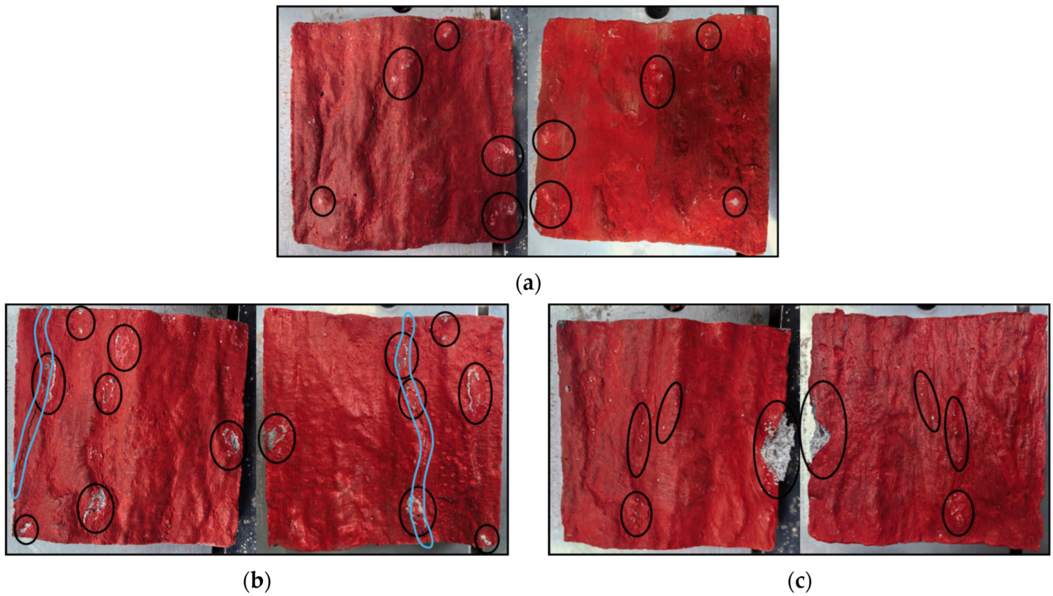
5.2. Verification of Damage Mechanism and Law of Strength Weakening

Figure 10 shows the surface morphology of the specimen after dynamic loading. When the peak dynamic load is 2 MPa, only a slight indentation appears on the discontinuity (black area in the figure), and there is no obvious crushing or cracking. When the peak dynamic load is 3.5 MPa, the indentation on the discontinuity deepens, and a certain degree of fragmentation occurs in the area with large undulations and cracking appearing along the fragmentation area (light blue area in the figure). When the peak dynamic load is 5 MPa, large pieces of material detach and fall away in areas with localized large undulations. Both sides of the discontinuity exhibit symmetrical distribution and matching damage. This illustration shows that a certain amount of damage occurs on both sides of the specimen discontinuity under the action of the dynamic load. As the peak dynamic load increases, the damage to the discontinuity becomes greater, which is consistent with the damage characteristics of the numerical simulation.

The energy generated during the specimen damage process is released in the form of elastic waves. For specimens in Group A3, a multichannel rock acoustic emission tester is used at the same time as the dynamic load to measure the energy released from the specimen and describe any damage that happened during the disturbance process. The results are shown in Figure 11.

The enlarged detail shows that during the rising stress stage of the triangular load, the normal stress increases linearly. The absolute energy release is relatively small, and the total energy release shows no obvious upward trend. This suggests that the rising phase released less total energy overall. Crack development within the specimen was subcritical, and the specimen primarily accumulated energy with minimal damage. Near the peak stress of the current cycle, the absolute energy release began to slowly increase with time.

Entering the falling stress stage, the normal stress shows a linear decrease, and the absolute energy release also reaches a peak after about one-sixth of the cycle is completed after the stress peak of the current cycle. At this time, the total energy release rises sharply. This indicates that the specimen gradually releases energy during the falling stage, and the peak of the absolute energy release is later than the peak of the normal stress, showing a damage hysteresis phenomenon. Discontinuity damage mainly occurs during this stage.

Overall, with the increase in the number of dynamic load cycles, the total energy release increases slowly, but the increase in each cycle is less than that in the previous cycle. The evolution of discontinuity damage in the numerical simulation has been analyzed above. Both demonstrate that energy accumulation dominates the rising stress stage, while energy release dominates the falling stress stage. There is also a damage hysteresis phenomenon, and this is also the main stage of discontinuity damage.

Table 11. Verification of strength weakening law in the laboratory test.

Degree of Dynamic Load Disturbance	The Shear Strength in Laboratory Test (MPa)	Shear Strength Weakening Coefficient (%)
Undisturbed	1.060
The peak dynamic load is 2 MPa	1.014	4.34
The peak dynamic load is 3.5 MPa	0.974	8.11
The peak dynamic load is 5 MPa	0.884	16.60

shows the shear strength and shear strength weakening coefficient of the discontinuity before and after a disturbance. The shear strength obtained from the laboratory test shows that the strength of the discontinuity after disturbance by dynamic loads is generally lower than that before disturbance. In addition, the larger the disturbance, the lower the shear strength, indicating that greater disturbances from dynamic loads further weaken the shear strength of the discontinuity. The law of variation for the weakening coefficient with the peak dynamic load is consistent with the law of variation for the shear strength weakening model obtained by the numerical simulation in the previous section.

6. Conclusions

This study distinguishes between the shear of discontinuities during dynamic load disturbance, which is generally considered, and the determination of the shear strength of discontinuities after dynamic load disturbance. This allows the damage to discontinuities caused only by dynamic load disturbance to be analyzed and the shear strength of discontinuities after damage weakening to be determined. This capability is the main innovation of this paper.

To achieve this research goal, the dominant controlling factors of dynamic load-induced discontinuity damage were analyzed using the discrete element method and the orthogonal design method. The damage mechanism was revealed by analyzing the macro and micro damage characteristics of rock discontinuities. Triaxial tests were performed on the simulated specimens after a disturbance to quantitatively characterize the shear strength weakening coefficient of the discontinuity after dynamic load disturbance. A post-disturbance strength weakening coefficient curve was obtained and verified by laboratory tests. The following conclusions were reached.

(1) A UDEC simulation specimen with discontinuity was created. The number of failure blocks and the crack growth length were used as damage indices in the Fish language. The five factors of the peak dynamic load, cycle number, dynamic loading frequency, discontinuity inclination angle, and discontinuity roughness all had a certain degree of influence on discontinuity damage. The orthogonal design method was used to carry out an analysis of the range and an analysis of variance, and it was determined that the dominant controlling factors for discontinuities in structures induced by dynamic loads are the dynamic loading frequency, peak dynamic load, and cycle number.

(2) Damage under dynamic loading mainly occurs at discontinuities. Each dynamic loading cycle is divided into two stages: rising stress and falling stress. In the rising stress stage, the rock discontinuities accumulate energy with shear cracks developing slightly and tensile cracks developing barely at all, resulting in relatively minor damage. In the falling stress stage, rebound deformation occurs in the direction of unloading, energy is released, and the dissipated energy slowly increases. After a period of time, both shear cracks and tensile cracks develop significantly, and the damage degree of the discontinuity increases, exhibiting a damage hysteresis effect, which eases with an increase in the cycle number.

(3) Dynamic load disturbance weakens the shear strength of the discontinuities compared to the undisturbed strength. The shear strength weakening coefficient is defined as the ratio of the decrease in shear strength after disturbance to the undisturbed strength. Based on the mathematical analysis, a model for the shear strength weakening of discontinuities after dynamic load disturbance has been established, considering the three dominant controlling factors: the dynamic loading frequency, peak dynamic load, and cycle number. The laboratory tests showed that the damage distribution and characteristics of discontinuities were basically consistent with the results of the numerical simulation analysis, and the law of strength weakening after dynamic loading was also consistent with the numerical simulation results. Extending the model of discontinuity shear strength weakening to a shear strength index weakening model, that is, a parameter correction of the shear strength index of the discontinuity after being disturbed by the dynamic load, can be applied in practical engineering and provide a reference for the engineering rock mass stability of discontinuities disturbed by a dynamic load.

References

1. Liu, C.Z. Genetic Types of Landslide and Debris Flow Disasters in China. Geol. Rev. 2014, 60, 858–868. [Google Scholar] [CrossRef]
2. Hong, Z.-J.; Si, K.; Li, Z.-H.; Zhu, C.; Du, F.; Cao, Z. Study on the Strength Characteristics of Sandstone Subjected to Coupled Static and Dynamic Loads from the Perspective of Microscopic Crack Propagation. Geomech. Geophys. Geo-Energy Geo-Resour. 2025, 11, 21. [Google Scholar] [CrossRef]
3. Liu, J.; Cong, Y.; Zhang, L.M.; Wang, Z.Q. Mesoscopic Damage Mechanism of Granite under True Triaxial Loading and Unloading. J. Cent. South Univ. (Sci. Technol.) 2021, 52, 2677–2688. [Google Scholar] [CrossRef]
4. Shi, Z.; Wu, C.; Li, X.; Xu, Y.; Li, K.; Sun, J. Dynamic Response and Energy Characterisation of High-Strength Sandstone under Progressive Cyclic Loading Based on Sustainable Mining. Appl. Sci. 2024, 14, 1101. [Google Scholar] [CrossRef]
5. Geranmayeh Vaneghi, R.; Ferdosi, B.; Okoth, A.D.; Kuek, B. Strength Degradation of Sandstone and Granodiorite under Uniaxial Cyclic Loading. J. Rock Mech. Geotech. Eng. 2018, 10, 117–126. [Google Scholar] [CrossRef]
6. Kim, J.-S.; Lee, C.; Kim, G.-Y. Estimation of Damage Evolution within an in Situ Rock Mass Using the Acoustic Emissions Technique under Incremental Cyclic Loading. Geotech. Test. J. 2021, 44, 1358–1378. [Google Scholar] [CrossRef]
7. Niktabar, S.M.M.; Rao, K.S.; Shrivastava, A.K.; Ščučka, J. Effect of Load Frequency and Amplitude of Displacement on Soft Synthetic Rock Joints under Cyclic Shear Loads. Bull. Eng. Geol. Environ. 2024, 83, 389. [Google Scholar] [CrossRef]
8. Soomro, M.H.A.A.; Indraratna, B.; Karekal, S. Critical Shear Strain and Sliding Potential of Rock Joint under Cyclic Loading. Transp. Geotech. 2022, 32, 100708. [Google Scholar] [CrossRef]
9. Peellage, W.H.; Fatahi, B.; Rasekh, H. Assessment of Cyclic Deformation and Critical Stress Amplitude of Jointed Rocks Via Cyclic Triaxial Testing. J. Rock Mech. Geotech. Eng. 2023, 15, 1370–1390. [Google Scholar] [CrossRef]
10. Peellage, W.H.; Fatahi, B.; Rasekh, H. Experimental Investigation for Vibration Characteristics of Jointed Rocks Using Cyclic Triaxial Tests. Soil Dyn. Earthq. Eng. 2022, 160, 107377. [Google Scholar] [CrossRef]
11. Siamaki, A.; Esmaieli, K.; Mohanty, B. Degradation of a Discrete Infilled Joint Shear Strength Subjected to Repeated Blast-Induced Vibrations. Int. J. Min. Sci. Technol. 2018, 28, 561–571. [Google Scholar] [CrossRef]
12. Gao, B.L.; Zhang, J.H.; Zhang, L.Q. Deterioration Characteristics of Structural Plane and Dynamic Instability Mechanism of High Dangerous Rock Mass under Earthquake. Earth Sci. 2022, 47, 4417–4427. [Google Scholar] [CrossRef]
13. Zheng, Z.; Li, R.; Pan, P.; Qi, J.; Su, G.; Zheng, H. Shear Failure Behaviors and Degradation Mechanical Model of Rockmass under True Triaxial Multi-Level Loading and Unloading Shear Tests. Int. J. Min. Sci. Technol. 2024, 34, 1385–1408. [Google Scholar] [CrossRef]
14. Li, J.; Guo, P.; Cui, H.; Song, S.; Zhao, W.; Chu, J.; Xie, W. Dynamic Response Mechanism of Impact Instability Induced by Dynamic Load Disturbance to Surrounding Rock in High Static Loading Roadway. Minerals 2021, 11, 971. [Google Scholar] [CrossRef]
15. Yousif, O.S.Q.; Karakouzian, M. Distinct Element Modeling of Uniaxial Compression Tests of Tuff-Like Lithophysal Material; Using Voronoi Tessellation System. Geotech. Geol. Eng. 2023, 41, 319–335. [Google Scholar] [CrossRef]
16. Akasheva, Z.K.; Bolysbek, D.; Assilbekov, B.; Yergesh, A.; Zhanseit, A.Y. Pore-Network Modeling and Determination of Rock and Two-Phase Fluid Flow Properties. Eng. J. Satbayev Univ. 2021, 143, 106–114. [Google Scholar] [CrossRef]
17. Du, J.; Huang, X.; Yang, G.; Xue, L.; Wu, B.; Zang, M.; Zhang, X. UDEC Modelling on Dynamic Response of Rock Masses with Joint Stiffness Weakening Attributed to Particle Crushing of Granular Fillings. Rock Mech. Rock Eng. 2023, 56, 1823–1841. [Google Scholar] [CrossRef]
18. Miao, C.; Liu, J.; Gao, M.; Li, J.; Pang, D.; Yuan, K. Insight into the Overload Failure Mechanism of Anchored Slope with Weak Structural Planes. Bull. Eng. Geol. Environ. 2024, 83, 390. [Google Scholar] [CrossRef]
19. Xu, W.; Hu, X.L.; Huang, L.; Zou, Z.X.; Ni, W.D.; Liu, X. Research on RQD of Rock Mass Calculated by Three-Dimensional Discontinuity Network Simulation Method and Its Accuracy Comparison. Chin. J. Rock Mech. Eng. 2012, 31, 822–833. [Google Scholar]
20. Shan, R.; Liu, N.; Sun, P.; Zhao, Z.; Dong, R.; Dou, H.; Meng, H.; Bai, Y. Experimental and Numerical Simulation Study of Rough Jointed Rock Samples under Triaxial Compression Conditions. Eng. Fract. Mech. 2025, 314, 110707. [Google Scholar] [CrossRef]
21. Li, K.; Yu, W.J.; Liao, Z.; Guo, H.X.; Pan, B.; Khamphouvanh, V.; Yang, J. A Laboratory-Testing-Tased Study on Mechanical Properties and Dilatancy Characteristics of Deeply Buried Mudstone under Different Stress Loading Rates. J. Coal Sci. Eng. China 2023, 48, 3360–3371. [Google Scholar] [CrossRef]
22. Wang, Y.; He, M. Numerical Investigation on Effect of Inclination and Position of Structural Planes on Rockbursts Triggered by Blasting Disturbance in Deep-Buried Tunnels. Rock Mech. Rock Eng. 2025, 58, 2739–2761. [Google Scholar] [CrossRef]
23. Zhang, Q.; Gu, Q.; Li, S.; Wang, H.; Han, G. A Shear Strength Criterion of Rock Joints under Dynamic Normal Load. Int. J. Rock Mech. Min. Sci. 2025, 186, 106002. [Google Scholar] [CrossRef]
24. Zhu, Q.; Yin, Q.; Tao, Z.; Yin, Z.; Jing, H.; Meng, B.; He, M.; Wu, S.; Wu, J. Shearing Characteristics and Instability Mechanisms of Rough Rock Joints under Cyclic Normal Loading Conditions. J. Rock Mech. Geotech. Eng. 2024, in press. [Google Scholar] [CrossRef]
25. Wang, K.X.; Xu, W.G.; Pan, Y.S.; Xue, J.Q.; Oparin, V.N.; Kiryaeva, T.A. Study on Tensile-Compression Damage and Fracture of Weak Interlayers in Block Rock Masses Induced by Quasi-Resonance. Chin. J. Rock Mech. Eng. 2025, 44, 114–127. [Google Scholar] [CrossRef]
26. Mashinskii, E.I. Elastic–Microplastic Nature of Wave Propagation in the Weakly Consolidated Rock. J. Appl. Geophys. 2014, 101, 11–19. [Google Scholar] [CrossRef]
27. Wang, W.; Wang, H.; Zhang, B.; Wu, Y.; Zhang, J.; Sun, D. Experimental Technique of Rock Multi-Strain Rates Dynamic and Static Load Superposition and Its Application. Rock Mech. Rock Eng. 2025, 58, 3159–3174. [Google Scholar] [CrossRef]
28. Barton, N. A Relationship between Joint Roughness and Joint Shear Strength. Proc. Int. Symp. Rock Mech. 1971, 1–8. Available online: https://www.researchgate.net/publication/296798762_A_relationship_between_joint_roughness_and_joint_shear_strength (accessed on 29 March 2025).
29. Barton, N.; Choubey, V. The Shear Strength of Rock Joints in Theory and Practice. Rock Mech. 1977, 10, 1–54. [Google Scholar] [CrossRef]
30. Jiang, Z.; Wang, L. The Affecting Factors of Slope Stability Based on Orthogonal Design. Adv. Mater. Res. 2013, 690–693, 756–759. [Google Scholar] [CrossRef]
31. Ni, Y.; Wang, R.; Leng, X.; Xia, F.; Wang, F. Modelling of Particle Flow Code Geotechnical Material Parameter Relationships Based on Orthogonal Design and Back Propagation Neural Network. Comput. Part. Mech. 2025, 12, 371–398. [Google Scholar] [CrossRef]
32. Sun, Z.; Han, Y.; Liu, F.; Min, R. Sensitivity Analysis of Influencing Factors of Vertical Bearing Capacity of Rock-Socketed Piles Based on Orthogonal Test. In Frontier Research on High Performance Concrete and Mechanical Properties; Xiang, P., Yang, H., Yan, J., Eds.; Springer Nature: Singapore, 2025; pp. 93–106. [Google Scholar]
33. Abdellah, R.; Bader, S.; Kim, J.-G.; Mohamed Ali, M. Numerical Simulation of Mechanical Behavior of Rock Samples under Uniaxial and Triaxial Compression Testsy. Min. Miner. Depos. 2023, 17, 1–11. [Google Scholar] [CrossRef]
34. West, I.; Walton, G. Quantitative Evaluation of the Effects of Input Parameter Heterogeneity on Model Behavior for Bonded Block Models of Laboratory Rock Specimens. Rock Mech. Rock Eng. 2023, 56, 7129–7146. [Google Scholar] [CrossRef]
35. Kim, J.; Kumpulainen, S.; Ferrari, A.; Pintado, X.; Laloui, L.; Heino, V. Salinity-Dependent Ultimate Shear Strength of Compacted Wyoming-Type Bentonite Investigated by Triaxial Tests. Appl. Clay Sci. 2024, 261, 107576. [Google Scholar] [CrossRef]
36. Jang, H.-S.; Zhang, Q.-Z.; Kang, S.-S.; Jang, B.-A. Determination of the Basic Friction Angle of Rock Surfaces by Tilt Tests. Rock Mech. Rock Eng. 2018, 51, 989–1004. [Google Scholar] [CrossRef]
37. Yang, S.Q.; Dai, Y.H.; Han, L.J.; Jin, Z.Q. Experimental Study on Mechanical Behavior of Brittle Marble Samples Containing Different Flaws under Uniaxial Compression. Eng. Fract. Mech. 2009, 76, 1833–1845. [Google Scholar] [CrossRef]
38. Vasyliev, L.; Malich, M.; Vasyliev, D.; Katan, V.; Rizo, Z. Improving a Technique to Calculate Strength of Cylindrical Rock Samples in Terms of Uniaxial Compression. Min. Miner. Depos. 2023, 17, 43–50. [Google Scholar] [CrossRef]
39. Yong, R.; Zhong, Z.; Du, S.G.; Zheng, S.; Zhang, Y.Y. Review on Research Advance of Basic Friction Angle of Rock Joints. Chin. J. Rock Mech. Eng. 2022, 41, 254–270. [Google Scholar] [CrossRef]
40. Li, W.; Ji, Z.S.; Dong, Z.Y.; Li, Z.L.; Li, Y. Vibration Analysis of Rock under Impact Loads Based on the Renormalization Method. J. Vib. Shock. 2016, 35, 49–54. [Google Scholar] [CrossRef]
41. Gao, X.; Jia, J.; Zhang, L.; Zhao, Y.; Tu, B. Mechanical Properties and Reasonable Proportions of Granite Similar Materials with Varying Degrees of Weathering. Environ. Earth Sci. 2025, 84, 140. [Google Scholar] [CrossRef]
Figure 1. Numerical simulation of a specimen with discontinuity and the parameter calibration.
Symmetry 17 00569 g001
Figure 2. Analysis results of range and variance. (a) Comparison analysis of the range of damage indexes for each factor; (b) comparison analysis of the variance of damage indexes for each factor.
Symmetry 17 00569 g002
Figure 3. The parameters change during dynamic load disturbance. (a) Variations in axial stress, total crack length, and dissipated energy; (b) variations in axial strain, shear cracks, and tensile cracks.
Symmetry 17 00569 g003
Figure 4. Distribution of damaged areas containing discontinuity specimens. (a) The distribution of macroscopic damage; (b) the distribution of failed blocks; (c) the distribution of crack propagation.
Symmetry 17 00569 g004
Figure 5. Contour plot of different parameters. (a) Contour plot of maximum principal stress. (The black arrows: Areas primarily subject to axial pressure. The white arrows: Areas primarily subject to tensile forces); (b) plot of damage distribution; (c) contour plot of local horizontal displacement. (The black circles: Non-contact areas on discontinuity. The white circles: Areas of contact and forces on discontinuity).
Symmetry 17 00569 g005
Figure 6. The process of obtaining shear strength of discontinuities. (a) Numerical simulation of the triaxial loading process; (b) calculation of shear strength.
Symmetry 17 00569 g006
Figure 7. Stress–strain curves of different dynamic loading peak values.
Symmetry 17 00569 g007
Figure 8. Variation rule of shear strength weakening coefficient with dominant controlling factors. (a) Variation rule of shear strength weakening coefficient with dynamic loading frequency; (b) variation rule of shear strength weakening coefficient with dynamic loading peak value under different numbers of cycles.
Symmetry 17 00569 g008
Figure 9. The main process of laboratory tests. (a) Specimens for laboratory tests; (b) equipment for laboratory tests; (c) loading process for laboratory tests.
Symmetry 17 00569 g009
Figure 10. Damage distribution of discontinuity. (a) A1: the peak dynamic load is 2 MPa; (b) A2: the peak dynamic load is 3.5 MPa; (c) A3: the peak dynamic load is 5 MPa. (The black circles: The fragmentation area of discontinuity. The blue circles: The cracks of discontinuity).
Symmetry 17 00569 g010
Figure 11. Dynamic load application process and energy release.
Symmetry 17 00569 g011