Multi-Granularity and Multi-Modal Feature Fusion for Indoor Positioning

Abstract

Despite the widespread adoption of indoor positioning technology, the existing solutions still face significant challenges. On one hand, Wi-Fi-based positioning struggles to balance accuracy and efficiency in complex indoor environments and architectural layouts formed by pre-existing access points (APs). On the other hand, vision-based methods, while offering high-precision potential, are hindered by prohibitive costs associated with binocular camera systems required for depth image acquisition, limiting their large-scale deployment. Additionally, channel state information (CSI), containing multi-subcarrier data, maintains amplitude symmetry in ideal free-space conditions but becomes susceptible to periodic positioning errors in real environments due to multipath interference. Meanwhile, image-based positioning often suffers from spatial ambiguity in texture-repeated areas. To address these challenges, we propose a novel hybrid indoor positioning method that integrates multi-granularity and multi-modal features. By fusing CSI data with visual information, the system leverages spatial consistency constraints from images to mitigate CSI error fluctuations while utilizing CSI’s global stability to correct local ambiguities in image-based positioning. In the initial coarse-grained positioning phase, a neural network model is trained using image data to roughly localize indoor scenes. This model adeptly captures the geometric relationships within images, providing a foundation for more precise localization in subsequent stages. In the fine-grained positioning stage, CSI features from Wi-Fi signals and Scale-Invariant Feature Transform (SIFT) features from image data are fused, creating a rich feature fusion fingerprint library that enables high-precision positioning. The experimental results show that our proposed method synergistically combines the strengths of Wi-Fi fingerprints and visual positioning, resulting in a substantial enhancement in positioning accuracy. Specifically, our approach achieves an accuracy of 0.4 m for 45% of positioning points and 0.8 m for 67% of points. Overall, this approach charts a promising path forward for advancing indoor positioning technology.

1. Introduction

In recent years, the demand for indoor positioning using mobile devices [1,2] has increased. This technology significantly enhances the navigational experience in expansive environments like shopping malls, supermarkets, airports, and train stations. Accurate indoor positioning is also crucial in vast indoor workspaces such as libraries, automated factories, and logistics warehouses, facilitating efficient scheduling and management of employees. In the livestock farming industry [3], precise indoor positioning of animals can greatly aid in activity tracking and monitoring, ultimately streamlining management practices and reducing labor costs.

Despite the advanced nature of GPS and Beidou satellite [4] positioning technologies, their usefulness is limited in indoor settings due to the inability of satellite signals to penetrate buildings. Furthermore, the intricacies of indoor environments, including walls, signal-obstructing objects, and the unrestricted movement of people, render traditional outdoor positioning systems ineffective for indoor applications. As a result, indoor positioning research has garnered significant attention in recent years.

Most indoor positioning methods currently rely on either Wi-Fi signals or image information. However, Wi-Fi-based positioning often struggles with accuracy, typically averaging over 1 m [5,6], and some methods require specific AP deployments that may only be feasible in some scenarios. On the other hand, visual positioning techniques utilizing image information offer improved precision but demand high-quality image data [7], often captured using stereo cameras. These powerful sensors are capable of capturing rich environmental information. However, visual positioning requires depth information, which is unavailable on standard smartphones equipped with monocular cameras.

As the capabilities of smartphones continue to evolve, the need for indoor positioning solutions tailored to these devices is growing. Given the limitations of smartphone cameras in capturing depth information, the current visual positioning techniques relying on stereo cameras are not widely applicable to the general public. Therefore, there is a compelling need for a multi-modal approach that leverages the capabilities of smartphone monocular cameras and seamlessly integrates them with Wi-Fi signals for positioning. Such a solution would greatly enhance positioning accuracy while reducing resource consumption, making it accessible and beneficial to many users.

In this context, this paper proposes an innovative multi-modal indoor positioning method combining coarse-grained and fine-grained features. This approach integrates the current mainstream Wi-Fi fingerprint positioning with visual positioning methods, leveraging the strengths of Wi-Fi fingerprints and image positioning through a coarse-to-fine-grained positioning strategy.

Specifically, this method employs a combination of coarse-grained and fine-grained approaches for positioning. In the coarse-grained stage, we use Wi-Fi data for positioning, reducing the computational complexity of fingerprint matching algorithms and improving computational efficiency. Simultaneously, we employ image data for coarse-grained positioning, effectively compensating for the shortcomings of Wi-Fi signals where CSI data are affected by multipath effects, leading to reduced accuracy. This stage primarily focuses on providing approximate location information, laying the foundation for subsequent positioning.

In the fine-grained stage, we fully use fine-grained CSI data to compensate for the lack of depth information in scale and distance in monocular image positioning. We establish a fused feature fingerprint library through deep integration of the features from Wi-Fi data and image data, further enhancing positioning accuracy. This stage primarily emphasizes precise adjustment and optimization of locations.

By employing this combined coarse-to-fine-grained multi-modal indoor positioning method, we not only enhance positioning accuracy but also address the limitation of smartphones being unable to perform visual positioning through binocular image capture. This method fully utilizes the smartphone’s hardware resources, eliminating the need for additional sensor equipment and offering advantages such as low cost and ease of popularization. Additionally, the method can adapt to various indoor environments and work scenarios, demonstrating high flexibility and scalability. Consequently, this method can provide ordinary users with more accurate, convenient, and reliable indoor positioning services, presenting extensive application prospects and market potential.

Two technical challenges must be tackled to achieve multi-modal indoor positioning with multiple granularities. The first challenge revolves around obtaining geometric relationships between images. We must employ effective methods to extract ample information from indoor scenes to accomplish this. This process can be delineated into two granularities: coarse-grained and fine-grained.

We consider leveraging a lightweight neural network like MobileVIT in the coarse-grained phase. Utilizing MobileVIT, we can extract features and classify data obtained from sensors, thereby completing the initial coarse positioning process. This neural network swiftly processes vast amounts of data and provides approximate scene information, which is pivotal for subsequent precise positioning. In the fine-grained phase, we further harness the distance and direction information derived from the coarse positioning stage. By considering the corresponding relationships of identical measurements in various spaces, we can accomplish coordinate mapping for enhanced positioning accuracy. This phase demands superior precision and intricate processing to ensure the integrity and reliability of the positioning outcomes.

The second challenge pertains to effectively amalgamating visual and Wi-Fi signals, the two information modalities. Our objective is to guarantee that the fused features yield improved positioning performance. We particularly contemplate the distance ratio between the target object and the camera’s visual boundary within the image space for data from a monocular camera. We employ the Scale-Invariant Feature Transform (SIFT) algorithm at the coarse-grained level to extract image features. SIFT’s scalability, facilitating its combination with other feature vectors, allows us to extract abundant and significant image features. At the fine-grained level, we meticulously assess the range of distance measurements within the user’s vicinity and address the limitations posed by CSI being influenced by multipath effects. To surmount these obstacles, we devise an ingenious technique capable of seamlessly fusing CSI and image features, generating a comprehensive fused feature fingerprint repository. Ultimately, we utilize the Support Vector Machine (SVM) approach for positioning, achieving high-precision and efficient indoor localization. This procedure illustrates the integration of coarse-to-fine granularities, ensuring precision and system efficiency.

Our three main contributions can be described in terms of coarse-grained and fine-grained aspects as follows:

Coarse-Grained: Proposing an Indoor Multi-Modal Positioning Strategy: We have developed a strategy to fully utilize scene images captured by a monocular camera in indoor environments. Through this approach, we can effectively extract users’ location information, laying the foundation for achieving high-precision indoor positioning.

Fine-Grained: Feature Fusion Method for Indoor Positioning: We introduce an innovative feature fusion method at the fine-grained level. This method effectively combines Wi-Fi and image features, generating a fused feature fingerprint library. We can provide more accurate and comprehensive indoor positioning information by integrating information from these two modalities.

Implementation and Evaluation of Positioning Method: We have not only remained at the theoretical and methodological level but have also implemented a practical positioning method and evaluated it in an indoor environment with mobile location points. The experimental results indicate that our solution achieves centimeter-level accuracy overall, with a specific 50th percentile error of less than 0.4 m for indoor targets. This level of accuracy demonstrates the effectiveness and practicality of our method.

The overall structure of this paper is as follows: Section 2 presents the research status of Wi-Fi-signal-based localization technology and image-based visual localization technology. Section 3 describes the CSI data used for multi-modal localization in Wi-Fi localization and the image data used for visual localization. Section 4 elaborates on the fusion localization of the data. Section 5 introduces the experimental environment and required equipment, analyzes the influence of relevant parameters on model performance, and provides a detailed analysis of the experimental results. Finally, in Section 6, we summarize our work.

2. Related Work

Positioning technology based on Wi-Fi signals and visual positioning technology based on images have garnered significant attention from scholars. Leveraging a multi-modal approach that utilizes one or multiple sensing modalities to determine indoor locations, building upon research in these indoor positioning technologies, has also gained traction among researchers. Numerous methods have been proposed in positioning systems, and these efforts can be broadly categorized into the following three categories.

2.1. Recent Advances and Challenges in Wi-Fi-Based Positioning Systems

In recent research on Wi-Fi indoor positioning, Meng et al. [8] utilized the Sequential Minimal Optimization (SMO) algorithm to establish a regression model between reduced-dimension features and corresponding locations, enabling location prediction. Zhang et al.’s [9] research provides new insights and methodologies for deep-learning-based Wi-Fi indoor positioning technology. By introducing trajectory CSI and utilizing deep learning models, the system is capable of achieving high-precision positioning in complex indoor environments. Chen et al. [10] proposed the Amplitude CSI Fingerprinting Localization (AmpFi) and Full-Dimensional CSI Fingerprinting Localization (FuFi) methods, which fully utilize the variability of subcarriers between different antenna pairs in MIMO systems and adopt the normalized amplitudes of full-dimensional subcarriers as fingerprints to achieve high-precision localization. Dai et al. [11] introduced CSI indoor positioning based on the K-nearest neighbor (KNN) algorithm. Still, this approach requires online comparison and matching with all data in the fingerprint library, resulting in inefficient positioning. Tian et al. [12] leveraged the clustering characteristics of CSI and applied the K-means clustering algorithm for feature extraction, followed by the KNN algorithm for positioning. Dang et al. [13] proposed an indoor positioning method using CSI with Support Vector Machine regression. These CSI-based indoor positioning methods typically consist of an offline stage for fingerprint library establishment and an online stage for fingerprint matching, ultimately achieving positioning. Xin et al. [14] presented the DFPhaseFL system, which extracts raw phase information from channel state information measurements, removes phase offsets to obtain filtered and calibrated phase information, and performs positioning. Ashraf et al. [15] proposed a magnetic field data-based indoor positioning method using magnetometers, but it is susceptible to electromagnetic interference, resulting in a decrease in positioning accuracy. Wu et al. [16] developed a Wi-Fi positioning system based on the Android platform that generates a fingerprint database and employs a weighted K-nearest neighbor algorithm for fingerprint matching and final location calculation. However, it does not effectively address the issue of RSSI volatility. Zhang et al. [17] proposed a new sensor node scheduling framework, but it requires a certain number of sensor nodes to be deployed and configured, resulting in high costs. Zhou et al. [18] introduced a WLAN indoor positioning method based on a manifold interpolation database, which constructs a fingerprint database using a combination of hybrid semi-supervised manifold learning and cubic spline interpolation. The method then calculates the location using the K-nearest neighbor algorithm. However, this approach requires prior deployment of access points (APs), and, when the number of APs is large, generating the fingerprint database can be time-consuming and complex. Moreover, these methods rely solely on Wi-Fi data, resulting in lower positioning accuracy than visual positioning and complicated AP deployment, which may not be suitable for all scenarios. In recent research on Wi-Fi indoor positioning, Meng et al. [8] utilized the Sequential Minimal Optimization (SMO) algorithm to establish a regression model between reduced-dimension features and corresponding locations, enabling location prediction. Chen et al. [10] proposed the Amplitude CSI Fingerprinting Localization (AmpFi) and Full-Dimensional CSI Fingerprinting Localization (FuFi) methods, which fully utilize the variability in subcarriers between different antenna pairs in MIMO systems and adopt the normalized amplitudes of full-dimensional subcarriers as fingerprints to achieve high-precision localization. Dai et al. [11] introduced CSI indoor positioning based on the K-nearest neighbor (KNN) algorithm. Still, this approach requires online comparison and matching with all the data in the fingerprint library, resulting in inefficient positioning. Tian et al. [12] leveraged the clustering characteristics of CSI and applied the K-means clustering algorithm for feature extraction, followed by the KNN algorithm for positioning. Dang et al. [13] proposed an indoor positioning method using CSI with Support Vector Machine regression. These CSI-based indoor positioning methods typically consist of an offline stage for fingerprint library establishment and an online stage for fingerprint matching, ultimately achieving positioning. Xin et al. [14] presented the DFPhaseFL system, which extracts raw phase information from channel state information measurements, removes phase offsets to obtain filtered and calibrated phase information, and performs positioning. Ashraf et al. [15] proposed a magnetic field data-based indoor positioning method using magnetometers, but it is susceptible to electromagnetic interference, resulting in a decrease in positioning accuracy. Wu et al. [16] developed a Wi-Fi positioning system based on the Android platform that generates a fingerprint database and employs a weighted K-nearest neighbor algorithm for fingerprint matching and final location calculation. However, it does not effectively address the issue of RSSI volatility. Zhang et al. [17] proposed a new sensor node scheduling framework, but it requires a certain number of sensor nodes to be deployed and configured, resulting in high costs. Zhou et al. [18] introduced a WLAN indoor positioning method based on a manifold interpolation database, which constructs a fingerprint database using a combination of hybrid semi-supervised manifold learning and cubic spline interpolation. The method then calculates the location using the K-nearest neighbor algorithm. However, this approach requires prior deployment of access points (APs), and, when the number of APs is large, generating the fingerprint database can be time-consuming and complex. Moreover, these methods rely solely on Wi-Fi data, resulting in lower positioning accuracy than visual positioning and complicated AP deployment, which may not be suitable for all scenarios.

2.2. Recent Advances in Image-Based Localization Techniques

In recent image localization research, visual positioning can rely on image feature extraction and matching methods, reducing visual positioning to an image-matching problem. This involves performing similarity matching between real-time images captured in the current moment and a pre-acquired set of training images. The matching image with high similarity corresponds to the location of the point to be positioned. Bai et al. [19] proposed a visual indoor positioning scheme based on landmarks using wearable devices. This approach involves wearing a customized image acquisition device on the chest and matching captured images against a pre-established database of natural landmarks in the building to obtain the user’s shooting location. Yang et al. [20] introduced a positioning method based on a monocular camera that efficiently utilizes feature points from visual information to solve for location and proposed a recursive algorithm to address displacement motion issues. Chen et al. [21] proposed a method based on location-aware convolutional neural networks for pothole detection in road images. However, the method lacks robustness against complex backgrounds. Martin et al. [22] presented a vision-based indoor positioning method incorporating a distance estimation algorithm in its image recognition system. Dryanovski et al. [23] proposed a fast visual positioning and ranging system using an RGB-D camera. This method recovers unconstrained six-degree-of-freedom camera trajectories by aligning sparse features observed in the current RGB-D image with previous feature models. Zhou et al. [24] developed a robot positioning method based on line detection, which extracts straight line features from images, applies transformations such as rotation and translation, determines the distance from the field of view center to the straight line, and achieves robot positioning. Alexander Buyval et al. [25] introduced an indoor visual positioning method based on particle filter segmentation and the nearest edge. This approach detects image edges and maps them to a 3D model of the room for positioning, eliminating the influence of factors such as texture noise on visual positioning. However, it requires the establishment of a 3D model before implementing positioning. Wu et al. [26] proposed a real-time positioning system based on detecting parking numbers. Its application range is limited, and it is not suitable for indoor use. Chen et al. [27] proposed a novel method for predicting future pedestrian locations using depth maps, 3D poses, and historical trajectories. However, the model has a high computational load and complexity. Fu et al. [28] proposed a bike-sharing electronic fence location optimization approach using a hybrid genetic annealing algorithm. It demands high standards for hardware installation and maintenance. Tacsyürek et al. [29] proposed DSHFS, a hybrid method that integrates a CNN, GeoServer, and TileCache to detect structures in large satellite images. Its complexity and data demands hinder real-time processing. Keil et al. [30,31,32,33,34,35] proposed 3D positioning, which is cost-prohibitive and reliant on specialized hardware, thus limiting its applicability in public spaces for the general populace.

2.3. Research Status of Fusion Data Localization

In recent data fusion research, Zhao et al. [36] proposed a positioning method that combines image data, readings from IMU sensors, and CSI information from Wi-Fi signals. This fusion approach improves positioning accuracy but still requires multiple modalities of data, resulting in limited generality. Dong et al. [37] used Wi-Fi fingerprints to select partitions from crowdsourced 2D photos collected by smartphones and constructed a 3D model. They identified path grids from user movements and compiled trajectory navigation for pedestrians. Fusion algorithms often achieve high indoor positioning accuracy but have high computational costs and more complex deployments. Chang et al. [38] introduced a hybrid model created during the modeling phase with Wi-Fi/cellular data connectivity, beacon signal strength, and a 3D spatial model. This method demands high experimental requirements and lacks generality.

In summary, algorithms that rely solely on Wi-Fi positioning typically have a positioning accuracy in the meter-level range, which is relatively low, and they often have high deployment requirements for access points (APs). On the other hand, algorithms that use image positioning generally require the creation of 3D image models, which can be resource-intensive. For multi-modal positioning, the image collection stage often requires acquiring data with depth information. However, regular smartphones typically use monocular cameras, which cannot capture depth information. Therefore, there are limitations and challenges associated with each positioning method, and further research and development are needed to overcome these limitations and improve positioning accuracy and efficiency.

3. Preliminary Aspects

Regarding preparatory work, we describe the CSI data used in Wi-Fi positioning for multi-modal localization and the image data employed in visual positioning.

3.1. Description of CSI Data

CSI serves as the data source for the positioning system, with its raw data in the form of complex matrices. The CSI Tool is employed to extract CSI data, with each CSI data packet capable of extracting 30 CSI subcarriers, which can be represented using matrices as follows:

$$\mathit{H}=\left[\begin{array}{cccc}\begin{array}{c}{h}_{11}\hfill \\ h_{21}\hfill \\ ⋮\hfill \\ h_{p1}\hfill \end{array}& \begin{array}{c}{h}_{12}\hfill \\ h_{22}\hfill \\ ⋮\hfill \\ h_{p2}\hfill \end{array}& \begin{array}{c}\cdots \hfill \\ \cdots \hfill \\ \\ \cdots \hfill \end{array}& \begin{array}{c}{h}_{1q}\hfill \\ h_{2q}\hfill \\ ⋮\hfill \\ h_{pq}\hfill \end{array}\end{array}\right],$$

(1)

where the configurations of each CSI data packet are $p\times q\times 30$, p denotes the number of transmitting antennas, q represents the number of receiving antennas, and the count of subcarriers is 30.

To effectively utilize CSI data, we thoroughly analyze the structure to extract the relevant data. Specifically, we define the CSI signal as

$${\mathit{H}}_{ij}=[{\mathit{H}}_1,{\mathit{H}}_2,\dots ,{\mathit{H}}_k].$$

(2)

Representing the amplitude on the K-th subcarrier as $∥{\mathit{H}}_k∥$ and the phase as $\angle {\mathit{H}}_k$, the CSI for each subcarrier can be expressed as

$${\mathit{H}}_k=∥{\mathit{H}}_k∥e^{j\angle {\mathit{H}}_k}.$$

(3)

As phase information is affected by frequency offset and cannot be accurately extracted, the proposed method only extracts amplitude values as fingerprint information as follows:

$${\mathit{H}}_k=[∥{\mathit{H}}_1∥,∥{\mathit{H}}_2∥,∥{\mathit{H}}_3∥,\dots ,∥{\mathit{H}}_k∥].$$

(4)

3.2. Image Data Description

The present study focuses on image data primarily acquired through monocular devices. These devices employ a single visual sensor to ascertain the positional data of targets within a given scene. The methods of positioning using monocular devices can be categorized based on the quantity of images utilized: single-image, dual-image, and multi-image positioning. For single-image positioning, the approach relies heavily on the calibration data of the camera and the correlation between artificial object markers in the physical environment and their corresponding representations in the captured image. This correlation facilitates the measurement of distance and orientation relative to the target object. In the case of dual-image positioning, the technique leverages the transformation of the camera’s coordinate system across two distinct viewpoints. Additionally, it considers the characteristic conversion between the camera’s coordinate system and an inertial coordinate system to extract pertinent distance and directional data. Multi-image positioning, on the other hand, employs mapping matrices that integrate multiple physical and image coordinate systems. This method incorporates camera calibration information to enhance the accuracy of position estimation.

Within image data analysis, the Scale-Invariant Feature Transform (SIFT) algorithm predominantly extracts salient features from the imagery, facilitating a comprehensive and nuanced understanding of the positional data obtained. SIFT is a local feature detection algorithm with several key advantages. Notably, it maintains robust invariance under image scaling, brightness changes, viewing angle variations, and image rotation conditions. The algorithm boasts feature descriptors that facilitate rapid matching and offer scalability by integrating other feature vectors. Fundamentally, SIFT operates by locating local feature points across spatial scales and employs feature descriptors with stable invariant properties for image matching. The extraction process of the SIFT algorithm comprises four primary steps: scale-space extrema detection, key point localization, orientation assignment, and descriptor generation.

3.3. Scale-Space Extremum Detection

Scale-space extremum detection provides theoretical support for extracting local invariant features from image data, and the Gaussian convolution kernel serves as a tool for achieving scale transformation. The convolution of an image with a Gaussian kernel results in a Gaussian pyramid, and constructing the scale space is

$$L(x,y,\sigma )=G{(x,y,\sigma )}^{*}I(x,y),$$

(5)

where $\sigma$ is the spatial scale factor, $L(x,y,\sigma )$ is the image scale space function, $I(x,y)$ is the original discrete two-dimensional image, $(x,y)$ is the image pixel coordinate, * is the convolutional spatial theory, and $G{(x,y,\sigma )}^{*}$ is the Gaussian kernel function, which is defined as

$$G(x,y,\sigma )={\displaystyle \frac{1}{2\pi {\sigma }^2}}{e}^{-\left(x^2+y^2\right)/2{\sigma }^2}.$$

(6)

The Difference of Gaussian (DoG) function is introduced to obtain effective feature points quickly in scale space. The DoG operator is obtained by subtracting images from adjacent Gaussian scale spaces, which is defined as

$$\begin{array}{c}\hfill D(x,y,\sigma )=\left(G(x,y,k\sigma )-G(x,y,\sigma )\right)\ast I(x,y)=L(x,y,k\sigma )-L(x,y,\sigma ).\end{array}$$

(7)

The SIFT algorithm generates an image pyramid corresponding to the general characteristics of the image; the smaller the scale, the less smooth the image, corresponding to the detailed characteristics of the image. After constructing the pyramid, finding the local extremum points in the scale space is necessary. The acquisition method is as follows: each pixel point is compared with eight neighboring points in the same scale domain and 9 points in the upper and lower adjacent scales, totaling $8+9\times 2=26$ pixel points. When the value of the detection point is the maximum or minimum value, it indicates that the point is the local extremum point in the scale space and two-dimensional image space, which is the feature point.

3.4. Key Point Positioning

In image pyramid computing, the DoG operator has strong edge effects, which leads to the detection of some extreme values that cannot be detected. Therefore, the detected local extreme values are not stable. It is necessary to further fit a three-dimensional quadratic function to screen the initially generated local extreme values to improve the accuracy of feature point localization, achieving accurate localization of the scale and position of the local extreme values.

Perform Taylor’s second-order expansion on the candidate extreme value points preliminarily determined as follows:

$$D\left(X\right)=D+{\displaystyle \frac{\partial D^T}{\partial X}}X+{\displaystyle \frac{1}{2}}{X}^T{\displaystyle \frac{\partial D^2}{\partial X^2}}X.$$

(8)

where $X={(x,y,\sigma )}^T$ partial derivatives of Equation (8) are calculated and set to 0, yielding the precise location and scale of the local extremum point:

$$\widehat{X}=-{\displaystyle \frac{{\partial }^2{D}^{-1}}{\partial X^2}}{\displaystyle \frac{\partial D}{\partial X}}.$$

(9)

Substituting the obtained value into the original equation, we can obtain

$$D\left(\widehat{X}\right)=D+{\displaystyle \frac{1}{2}}{\displaystyle \frac{\partial D^T}{\partial X}}\widehat{X}.$$

(10)

This value represents the offset of the local feature point relative to the interpolation center, so, when the offset is less than a certain threshold, the point is discarded and vice versa.

At the same time, using the Hessian matrix to detect unstable local extrema at the edge, the obtained local extrema are more accurate, enhancing the stability of the feature matching in the positioning system while improving the anti-noise performance of the system. The theoretical basis is that the principal curvature of the DoG operator’s extrema is larger on the edge span, while the principal curvature in the perpendicular direction to the edge is smaller. By setting a certain threshold, unstable local feature points on the edge can be removed to improve the instability of the differential operator at image edges. The $2\times 2$ Hessian matrix can be used to obtain the principal curvature of the differential operator:

$$H=\left[\begin{array}{cc}{D}_{xx}& D_{xy}\\ D_{yx}& D_{yy}\end{array}\right].$$

(11)

where D is the difference between adjacent pixel points. The eigenvalues of H are proportional to the principal curvatures of local extrema. Let the maximum and minimum values of H be $\alpha$ and $\beta$, respectively. In physical terms, $\alpha$ represents the gradient value in the X direction, and $\beta$ represents the gradient value in the Y direction. Then, the trace $Tr$$\left(H\right)$ and determinant value $Det$$\left(H\right)$ of matrix H can be obtained as follows:

$$\begin{array}{cc}\hfill Tr\left(H\right)& =D_{xx}+D_{yy}=\alpha +\beta ,\hfill \\ \hfill Det\left(H\right)& =D_{xx}{D}_{y{y}^{\prime }}-{\left(D_{xy}\right)}^2=\alpha \beta .\hfill \end{array}$$

(12)

Let $\gamma =\alpha /\beta$, the principal curvature of the local extreme value on the edge, be defined as

$${\displaystyle \frac{Tr{\left(H\right)}^2}{Det\left(H\right)}}={\displaystyle \frac{{(\alpha +\beta )}^2}{\alpha \beta }}={\displaystyle \frac{{(\beta \gamma +\beta )}^2}{\gamma {\beta }^2}}={\displaystyle \frac{{(\gamma +1)}^2}{\gamma }}.$$

(13)

From Equation (13), it can be seen that the magnitude of the principal curvature is only affected by the ratio of $\alpha$ and $\beta$. When and only when $\alpha$ and $\beta$ are equal, the principal curvature takes the minimum value, and the principal curvature is positively correlated with $\gamma$ and decreases as $\gamma$ decreases. The above analysis shows that the principal curvature of the image edge extreme point is large; that is, the value of $\gamma$ is large. To remove unstable points, let T be the threshold value. If the measured extreme point satisfies the following conditions, then the extreme point is retained. Otherwise, it is deleted, as shown in

$${\displaystyle \frac{Tr{\left(H\right)}^2}{Det\left(H\right)}}<{\displaystyle \frac{{\left(T_{\gamma }+1\right)}^2}{T_{\gamma }}}.$$

(14)

3.5. Determine the Direction of the Key Point

The SIFT feature has good rotational invariance, mainly because each identified feature point has a dominant direction determined by the gradient distribution characteristics of individual pixel points within the DOG scale space neighborhood. The gradient magnitude and direction of the pixel point at image $(x,y)$ location are represented as

$$\begin{array}{cc}\hfill A(x,y)& =\sqrt{{\left(L(x+1,y)-L(x-1,y)\right)}^2+{\left(L(x+1,y+1)-L(x-1,y-1)\right)}^2}\hfill \\ \hfill \theta (x,y)& =arctan{\displaystyle \frac{L(x,y+1)-L(x,y-1)}{L(x+1,y)-L(x-1,y)}},\hfill \end{array}$$

(15)

where $L(x,y)$ represents the grayscale value of the feature point in the corresponding scale space, $A(x,y)$ represents the magnitude of the gradient, and $\theta (x,y)$ represents the direction of the gradient.

3.6. Feature Descriptor Construction

The above steps have determined the key information of each feature point $L(x,y,\sigma ,\theta )$: location, scale, and direction. Next, it is necessary to establish a descriptor for each key point, using a set of vectors to describe the key point so that it does not change with various changes, such as changes in lighting and perspective. This descriptor not only includes the key point but also includes the pixels around the key point that contribute to it, and the descriptor should have high uniqueness to improve the probability of correct matching of feature points. In the actual calculation process, to enhance the robustness of the matching, $4\times 4=16$ seed points are used to describe each key point, which can generate 128 data for a key point, resulting in a 128-dimensional feature vector.

4. Multi-Modal Localization

4.1. Proposed Method

The system framework is shown in Figure 1, which is divided into two online and offline stages. In the offline stage, we collect image data and Wi-Fi data. Firstly, image data are collected in the coarse-grained stage and then trained using the MobileVit lightweight network. After training, the images are matched with those in the database. Due to the high accuracy of location acquisition relying only on image positioning but also the high accuracy rate of positioning in large-precision situations, after coarse positioning blocking, we extract features from the collected images and fuse them with the features of CSI to establish a new fused feature fingerprint library. Finally, model training is performed to obtain location information.

The online stage is responsible for positioning. We input the coordinates’ Wi-Fi data and image data to be predicted into the system. Firstly, the image is used for coarse positioning blocking, and then the sift algorithm is used to extract features from the image data and fuse them with the Wi-Fi data. Finally, a trained SVM model matches the features with those in the fused feature fingerprint library.

This system framework design aims to improve the accuracy and reliability of location information by combining image data and Wi-Fi data, as well as utilizing advanced algorithms and models for feature extraction and matching, thereby achieving precise positioning in the online stage.

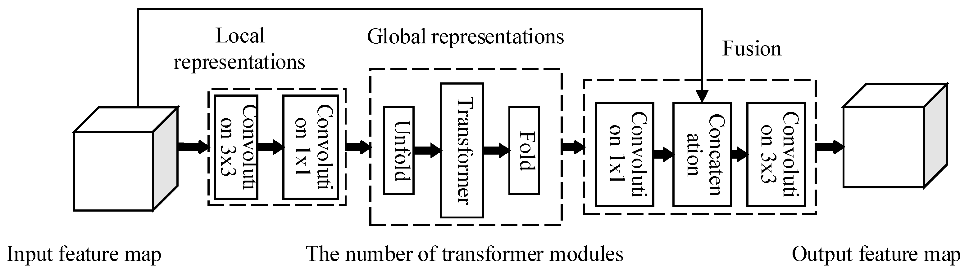
4.2. Coarse-Grained Location Is Conducted by Mobilevit Network

The MobileViT module uses standard convolution and transformer mechanisms to learn local and global information in the feature map. Its structure is shown in Figure 2. Assuming that the input feature map X of the MobileViT module has a size of $H\times W\times C$ (H is the height of the input feature map, W is the width of the input feature map, and C is the number of channels of the input feature map), a 3 × 3 convolution kernel is used to model the local spatial information in the feature map. Next, a 1 × 1 convolution maps the feature map to a higher-dimensional feature space to enrich the semantic information learned by the convolution.

After two convolution operations, the input feature map X is transformed into a local feature map of equal size. Then, $X_L$ is divided into N equal-sized image blocks, each containing P pixels, which are then expanded into a set of feature sequences $X_U$ of size $P\times N\times d$ to learn global semantic information in the feature map, where $P=w\times h$, $N=(H\times W)/P$ (W and H are the width and height of the preset image blocks, and d is the feature dimension). The pixel features at the same location between different image blocks in $X_U$ are processed by consecutive groups of transformer modules to obtain the global feature sequence $X_G$ as follows:

$$X_G\left(p\right)=\mathrm{Transformer}\left(X_U\left(p\right)\right),1\le p\le P.$$

(16)

Unlike the original visual transformer, MobileViT does not lose the positional information between the internal pixels and the image block. Therefore, there is no need for positional encoding to add positional information. Afterward, $X_G$ is folded to obtain the feature map $X_F$, which has a size of $H\times W\times d$. The unfolding and folding operations above are implemented by combining the Transpose and Reshape functions. Then, $X_F$ is convolved and mapped to a size of 1 × 1 to the same dimension C as the input feature map X of the MobileViT module. At this point, the size of $X_F$ is $H\times W\times C$, which can be concatenated with the input feature map X to form a new feature map with a dimension of 2C. Finally, a 3 × 3 convolution kernel is used to fuse the parallel new feature maps, and the dimension of the new feature map is mapped back to C.

In practical applications, indoor scenes are less affected by weather and seasons, and changes in light intensity do not cause as much change in the environment’s appearance as outdoor scenes. Moreover, indoor environments have distinct line structures, and occlusion interference is more common. Therefore, in indoor application scenarios, more attention must be paid to the impact of environmental occlusion and perspective changes on location recognition, and specialized indoor scene datasets are needed to train the network. It contains 100 locations in indoor scenes, each with 8 orientations, and each orientation has 11 heights, with a total of 8800 images collected. During the training process, the original image with any aspect ratio is resized to a size of 227 (long) × 227 (wide) and then sent to the convolutional layer. Finally, after integrating the results of each convolutional layer through the fully connected layer, the output result is mapped to the corresponding category probability space by the transformer’s SoftMax layer.

Let $I_i$ represent the input image and $\theta$ represent the parameters of the entire network. The output of the fully connected layer can be expressed as

$$x_i=f\left(I_i,\theta \right).$$

(17)

$x_i$ is normalized and mapped to the probability space by the SoftMax function, and the final output of the trained network is

$$\sigma \left(x_i^j\right)={\displaystyle \frac{e^{x_i^j}}{{\sum }_{k=1}^n{e}^{x_i^k}}},j=1,2,\cdots ,n.$$

(18)

where n is the number of regions in the indoor scene, and $\sigma \left(x_{ij}\right)$ represents the probability that the j image belongs to the i-th region, satisfying the following relationship

$$\sigma \left(x_i^1\right)+\sigma \left(x_i^2\right)+\cdots +\sigma \left(x_i^n\right)=1.$$

(19)

During the backpropagation training process, the network parameters are optimized using the SoftMax loss function, which is defined as follows:

$$L_{\theta }^1=-\sum _{j=1}^n{y}_i·log\sigma \left(x_i^j\right),$$

(20)

where $y_i$ is the label of the training data.

In the aforementioned description, we elaborated on the forward propagation process of the network. Specifically, the input image $I_i$ and network parameters $\theta$ undergo a series of computations, ultimately outputting a feature vector $x_i$ from the fully connected layer. Subsequently, the SoftMax function maps $x_i$ to the probability space, where $\sigma \left(x_i^j\right)$ represents the probability that image j belongs to the i-th indoor scene region. This step ensures that the sum of all probabilities is 1, satisfying the fundamental property of probability distributions:

$$\sigma \left(x_i^1\right)+\sigma \left(x_i^2\right)+\cdots +\sigma \left(x_i^n\right)=1.$$

(21)

During the backpropagation training phase of the network, we employ the SoftMax loss function $L_{\theta }^1$ to optimize the network parameters. This loss function measures the performance of the model by comparing the predicted probability distribution with the true label $y_i$. Specifically, the loss function computes the sum of the logarithmic losses for the predicted probabilities corresponding to the true labels and takes its negative value as the final loss:

$$L_{\theta }^1=-\sum _{j=1}^n{y}_i·log\sigma \left(x_i^j\right),$$

(22)

where $y_i$ is the label of the training data. This design aims to minimize prediction errors, thereby improving the model’s prediction probability for true labels.

It is worth noting that the SoftMax loss function not only considers the prediction probability of the correct class but also enhances the model’s discrimination ability for class boundaries by penalizing the probabilities of other incorrect classes. This mechanism allows the model to continuously adjust its parameters during training to more accurately identify different scene regions.

Our locally curated dataset encompasses a comprehensive collection of images. Specifically, we have meticulously captured images from 100 unique and strategically selected location points within the designated area. At each of these location points, we have ensured a diverse representation by capturing a total of 88 images, varying both in orientation and height. This meticulous approach not only ensures a rich dataset but also captures the nuances and subtleties of the environment from multiple perspectives. In aggregate, our dataset boasts a total of 8800 high-quality images, each contributing to a holistic and comprehensive understanding of the target area. In Figure 3, we have meticulously presented image data from each location point, showcasing 8 distinct orientations.

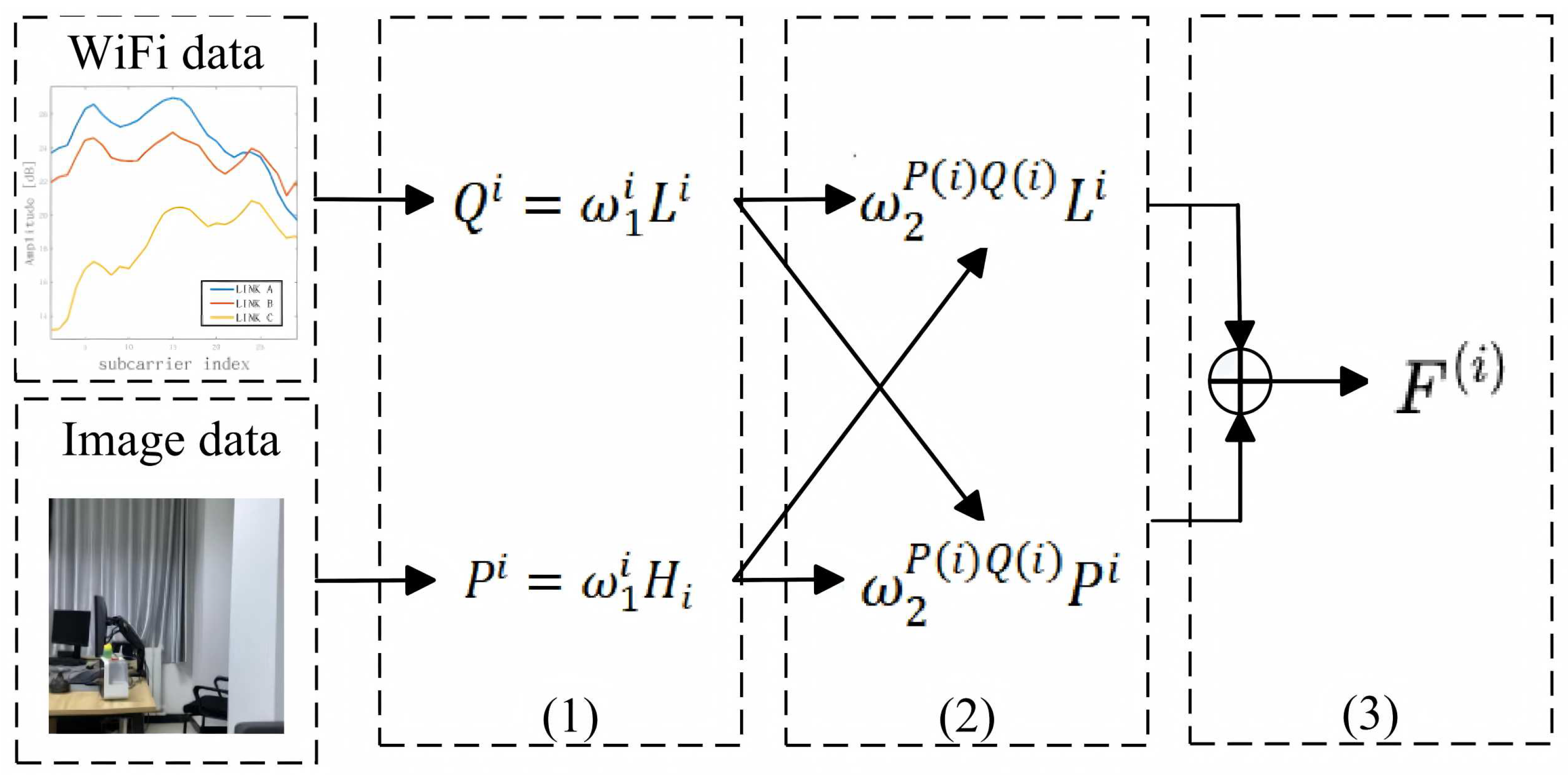
4.3. Improved Feature Fusion Method

An original scene image extracted by the SIFT algorithm is denoted as $L(x,y,\sigma ,\theta )$, where $(x,y)$ represents the location, $\sigma$ represents the scale, and $\theta$ represents the direction. Therefore, the feature of the i image is denoted as $L^i$.

The amplitude on the i subcarrier of the CSI data is represented as $∥{\mathit{H}}_i∥$, and the phase is represented as $\angle {\mathit{H}}_i$. Therefore, the CSI on each subcarrier can be represented as

$${\mathit{H}}_i=∥{\mathit{H}}_i∥e^{j\angle {\mathit{H}}_i}.$$

(23)

Directly fusing different image features without any preprocessing process can easily produce interference information and may harm the fused features. To reduce noise, first, standardize the image feature vectors using

$$Q^i={\omega }_1^i{L}^i,$$

(24)

where ${\omega }_1^i$ is defined as

$${\omega }_1^i={\displaystyle \frac{max\left(L^i\right)-{\mu }_1^i}{{\sigma }_1^i}},$$

(25)

where ${\mu }_1^i$ and ${\sigma }_1^i$ are the mean and standard deviation of $L^i$, respectively.

The CSI features are standardized similarly, and the normalized CSI feature vector is

$$P^i={\omega }_1^i{H}_i,$$

(26)

where ${\omega }_1^i$ is defined as

$${\omega }_1^i={\displaystyle \frac{max\left(P^i\right)-{\mu }_1^i}{{\sigma }_1^i}},$$

(27)

where ${\mu }_1^i$ and ${\sigma }_1^i$ are the mean and standard deviation of $P^i$, respectively. The improved fusion model can better utilize each fused feature and highlight the information in each feature vector. It makes the extracted feature description more accurate and comprehensive and multiplies different feature vectors of the image together; that is, $P^i$ and $Q^i$ are multiplied together to generate a fused feature $S^i$, defined as follows:

$$S^{P\left(i\right)Q\left(i\right)}=P^i\odot Q^i,$$

(28)

where ⊙ represents multiplying the elements of the input vector S element by element and then processing the resulting vector to obtain the final fused vector $F^i$

$$F^i={\displaystyle \frac{1}{2}}\left({\omega }_2^{P\left(i\right)Q\left(i\right)}{L}^i+{\omega }_2^{P\left(i\right)Q\left(i\right)}{P}^i\right),$$

(29)

where ${\omega }_2^{P\left(i\right)Q\left(i\right)}$ is defined as

$${\omega }_2^{P\left(i\right)Q\left(i\right)}={\displaystyle \frac{max\left(S^{P\left(i\right)Q\left(i\right)}\right)-{\mu }_2^{P\left(i\right)Q\left(i\right)}}{{\sigma }_2^{P\left(i\right)Q\left(i\right)}}},$$

(30)

where ${\mu }_2^{P\left(i\right)Q\left(i\right)}$ and ${\sigma }_2^{P\left(i\right)Q\left(i\right)}$ represent the mean and standard deviation of $S^{P\left(i\right)Q\left(i\right)}$.

After obtaining the fused feature F, generate a coordinate set $\mathit{P}$ corresponding to the coordinates as

$$\mathit{P}=\{(x_1,y_1),(x_2,y_2),\cdots ,(x_n,y_n)\}.$$

(31)

The flowchart of the fusion algorithm is shown in Figure 4.

Establish a fused feature fingerprint set k as

$$k=\{F_1,F_2,\cdots ,F_n\}.$$

(32)

where n represents the number of samples; that is, each fingerprint database contains n fused features. The n fused feature fingerprints contained in the fingerprint set k are, respectively, mapped to coordinates to generate a fused feature fingerprint database K as

$$K=\{(F_1,(x_1,y_1)),(F_2,(x_2,y_2)),\cdots ,(F_n,(x_n,y_n))\},$$

(33)

where $F_n,(x_n,y_n)$ represents the fused feature information of the n sample and the coordinate information of the horizontal axis x and the vertical axis y.

4.4. Train the SVM Model for Positioning

Based on the fused feature fingerprint library, an SVR regression model is established for positioning. The core idea of the SVR regression algorithm is to use regression to find the relationship between the fused feature vector $F^i$ and the location. In high-dimensional space, a nonlinear mapping method is used to find an optimal hyperplane to replace the original nonlinear relationship.

Based on the SVR algorithm, using the relationship between the amplitude information and the coordinate information of CSI, establish functions $f_x$ and $f_y$. Establish a linear regression estimation function on the axis as

$$x=〈\mathit{w},\phi \left(r\right)〉+b,$$

(34)

where $\mathit{w}$ is the weight vector, $\phi \left(r\right)$ maps the low-dimensional CSI fingerprint information to a high-dimensional space, and b is a constant value.

The SVR is $\epsilon$-SVR ($\epsilon$ insensitive support vector algorithm), and the risk generalization function $R\left(\omega \right)$ of SVR is

$$R(\omega )=\mathit{\int }max\left(\right|f(CSI,\mathit{w})-x|-\epsilon ,0)\mathrm{d}F(CSI,x).$$

(35)

To minimize the loss when determining parameters w and b, the optimization problem can be defined as

$$f\left(\mathit{w}\right)={\displaystyle \frac{1}{2}}{∥\mathit{w}∥}^2+C\left(\sum _{i=1}^L{\xi }_i+\sum _{i=1}^L{{\xi }_i}^{*}\right).$$

(36)

The constraint condition is

$$\left\{\begin{array}{c}(〈\mathit{w},\phi \left(r\right)〉+b)-x_i\le \epsilon +{\xi }_i\hfill \\ x_i-(〈\mathit{w},\phi \left(r\right)〉+b)\le \epsilon +{{\xi }_i}^{*}\hfill \\ {{\xi }_i}^{*}\ge 0,{\xi }_i\ge 0,i=1,2,\dots ,L.\hfill \end{array}\right.$$

(37)

where ${∥\mathit{w}∥}^2$ represents the complexity of the learning function. Introducing ${\displaystyle \sum _{i=1}^L}{\xi }_i+{\displaystyle \sum _{i=1}^L}{{\xi }_i}^{*}$ as a slack variable allows some samples to be outside the interval band. Then, using the dual principle, the linear representation of the set of $\mathit{w}$ support vectors is

$$\mathit{w}=\sum _{i\in SV}{\gamma }_i\varphi \left(CS{I}_i\right).$$

(38)

We obtain

$$x=\sum _{i\in SV}{\alpha }_i〈\phi \left(r_i\right),\phi \left(r\right)〉+b.$$

(39)

The relationship between CSI fingerprint information and coordinates is nonlinear; thus, the Gaussian kernel function $K(r_i,r)$ is used instead of $〈\phi \left(r_i\right),\phi \left(r\right)〉$ as follows:

$$x=\sum _{i\in SV}{\alpha }_{i}K(r_i,r)+b.$$

(40)

The calculation function for the x-axis and y-axis coordinates is obtained from Equation (40). When the predicted position is different from the actual position, there is an error. Let the predicted point coordinates be $(x,y)$ and the actual coordinates be $(x_1,y_1)$. The linear distance between the predicted point coordinates and the actual coordinates is $Dis$, which is used to represent the error, as follows:

$$Dis=\sqrt{{(x_1,y_1)}^2-{(x,y)}^2}.$$

(41)

The overall multi-granularity, multi-modal indoor localization process is illustrated in Algorithm 1:

Algorithm 1 Indoor positioning method based on multi-granularity and multi-modal features

Input: Image set $I=\{1,2,3,\dots ,n\}$; mobile phone movement distance D between two fixed shooting points; Wi-Fi signal of the location; Output: The coordinate range of the image; the predicted location 1: Acquire image data based on the monocular camera of the mobile phone and camera calibration; 2: Through the MobileVit algorithm, determine the matching area for image feature detection; 3: Extract the image feature $L(x,y,\sigma ,\theta )$ through the SIFT algorithm, and extract the CSI amplitude feature ${\mathit{H}}_i=∥{\mathit{H}}_i∥e^{j\angle {\mathit{H}}_i}$; 4: Standardize the image features and CSI amplitude features separately, with image features $Q^i={\omega }_1^i{L}^i$ and CSI amplitude features $P^i={\omega }_1^i{H}_i$; 5: Extracted features are fused to generate a fused vector F, where $F^i={\displaystyle \frac{1}{2}}\left({\omega }_2^{P\left(i\right)Q\left(i\right)}{L}^i+{\omega }_2^{P\left(i\right)Q\left(i\right)}{P}^i\right)$; 6: Generate the fused fingerprint database $K=\{(F_1,(x_1,y_1)),(F_2,(x_2,y_2)),\dots ,(F_n,(x_n,y_n))\}$; 7: Train the SVM model using the fused fingerprint database; 8: Take a picture of the indoor scene at the point to be predicted, and perform region matching again by following steps 1 and 2; 9: Collect Wi-Fi signals of the points to be predicted, perform steps 3–5 to extract image features, and perform feature fusion; 10: Input the fused features to the SVM model trained in step 7 for feature matching; 11: Output the predicted position and measure the error $Dis=\sqrt{{(x_1,y_1)}^2-{(x,y)}^2}$.

5. Experimental Analysis and Verification

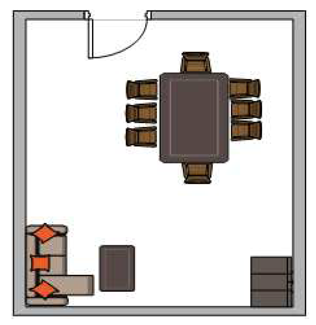
5.1. Experimental Environment Setup

The experiment used a desktop computer as the acquisition terminal during the data acquisition stage. The desktop computer runs a 32-bit Ubuntu Server 10.04(LTS) operating system equipped with an Intel 5300 802.11n wireless network card (Intel Corporation, Santa Clara, CA, USA). The AP (or monitor) communicates with users using the interface wlan0 running on channel 6 in the 2.4 GHz band and communicates with the server using the interface eth0. The server uses eth1 to connect to the Internet. During the data processing stage, the CPU of the laptop is Core i7-11800H@2.30 GHz (Intel Corporation, Santa Clara, CA, USA), and the operating system is Ubuntu 20.04.3. The laboratory layout is shown in Figure 5, with 100 points of Wi-Fi data and image data collected, with a distance of 0.4 m between adjacent points.

5.2. Comparison of Coarse-Grained Positioning Experiments

In coarse-grained localization experiments, we employed the classification strategy of MobileViT. Initially, the network was trained on a local test set, followed by testing.

Table 1. Accuracy of rough classification under different categories.

Area Classification	Location Points Included in Each Category	Sample Quantity in Each Category	Classification
100 categories	1	1 × 88	38.31%
10 categories	5	5 × 88	88.23%
Category 6	16	16 × 88	96.48%
Category 2	50	50 × 88	99.34%

lists the experimental results revealed when each location was treated as a separate class for recognition. The average recognition accuracy was only 38.31%. However, the accuracy improved when we adopted a regional blocking recognition approach. Specifically, dividing every 10 points into a region resulted in ten regions (or ten classes), achieving a recognition accuracy of 88.23%. Furthermore, when using 16 points as a region, six regions (or six classes) were formed, each containing 1444 photos, achieving an impressive recognition accuracy of 96.48%.

To more comprehensively evaluate the performance of the proposed algorithm, we conducted experimental comparisons with ResNet and MobileViT networks. As shown in

Table 2. Accuracy of rough classification under different algorithms.

Model	Categories
	2	6	10
ResNet	91.88%	79.74%	65.21%
MobileNet	95.60%	89.86%	72.83%
MobileVit	99.34%	96.48%	88.23%

, the classification accuracy of the MobileViT network was 96.48%, which was significantly higher than that of the ResNet network. These results demonstrate the superior performance and higher classification accuracy of the MobileViT network in coarse-grained localization tasks.

5.3. Comparison of Fine-Grained Positioning Experiments

To evaluate the performance of the proposed algorithm in fine-grained scenarios, we conducted a series of comparative experiments under various conditions. Initially, we compared our method against a baseline localization approach that relies solely on Wi-Fi data, aiming to establish a benchmark for comparison. Subsequently, we performed additional experiments using varying sample sizes and different antenna configurations to assess the impact of these factors on the algorithm’s performance. Furthermore, we benchmarked our algorithm against other popular existing methods to provide a broader perspective on its relative performance.

In this paper, we utilized cumulative distribution function (CDF) plots to visualize the distribution of localization errors and their magnitudes. By examining the cumulative probability distribution of localization errors and calculating the average error, we could quantitatively evaluate the experimental results and provide a comprehensive assessment of the algorithm’s performance. This approach allowed us to gain insights into the algorithm’s behavior and identify potential areas for improvement.

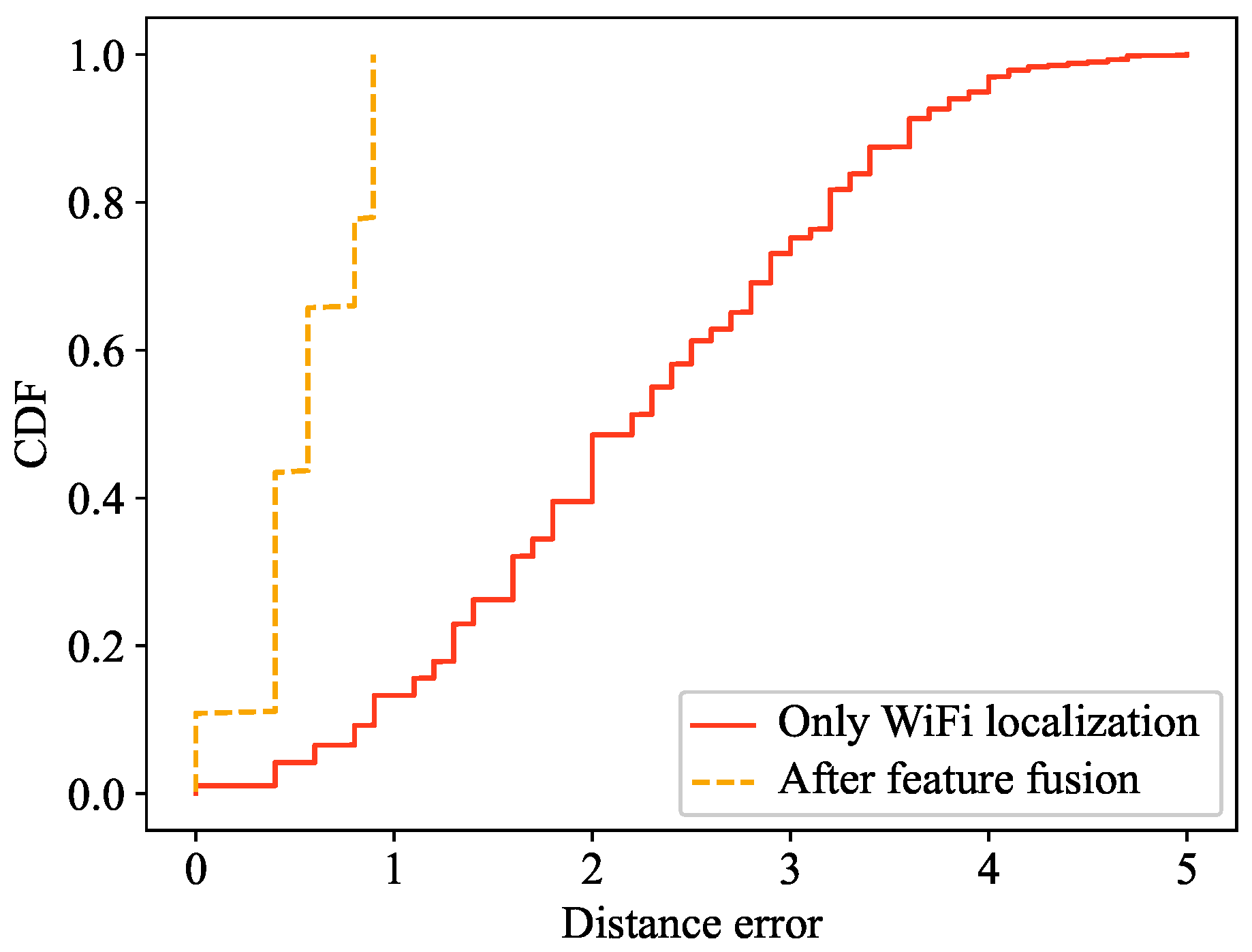
5.4. Comparison with the Method Without Image Data and Only Using Wi-Fi Data for Positioning

Comparing the proposed method with a Wi-Fi localization approach that does not incorporate coarse-to-fine positioning strategies and feature fusion data reveals significant differences in performance. As illustrated in Figure 6, our method achieves a 50% localization error within 1 m, whereas the approach relying only on Wi-Fi data has a 50% localization error within 2 m. The strategies and techniques introduced in this paper offer substantial advantages over the Wi-Fi-only localization method, demonstrating improved accuracy and precision.

5.5. Comparison of Experiments with Different Sample Sizes

To further explore the impact of varying sample sizes on the performance of our algorithm, we conducted a comparative analysis in Figure 7 using 5000, 10,000, and 20,000 samples. The experimental results reveal that, with 5000 samples, 50% of the localization errors are within 1.2 m. When the sample size is increased to 10,000, the 50% localization error threshold improves to within 0.8 m. However, with a substantial increase to 20,000 samples, the algorithm exhibits remarkable performance, with 50% of localization errors narrowing down to within just 0.4 m. As the sample size increases, the performance of our algorithm improves significantly, with the most optimal results observed when using 20,000 samples.

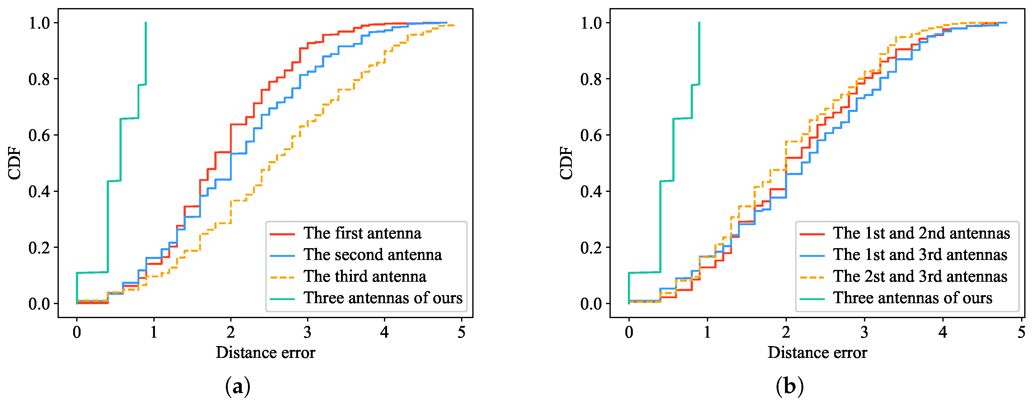
5.6. Comparison with Different Antenna Numbers

To evaluate the effect of antenna quantity on the performance of our algorithm, we conducted a comparative analysis using both single and multiple antennas. We employed CDF plots to represent the errors across different sample sizes, as demonstrated in Figure 8. In our experiment, we utilized three antennas and compared their performances solely relying on Antenna 1, Antenna 2, or Antenna 3. Furthermore, we compared the results obtained using two antennas, specifically comparing the methods that employed Antennas 1 and 2, Antennas 2 and 3, and Antennas 1 and 3. This comprehensive analysis allowed us to assess the impact of varying antenna configurations on the algorithm’s performance.

To clarify, when utilizing a single antenna, specifically Antenna 1, the localization errors for 50% of the data points fall within a radius of 1.8 m. Similarly, when relying on Antenna 2, the same percentage of errors are contained within 2.1 m, and, with Antenna 3, the errors remain within 2.4 m for 50% of the cases. When incorporating two antennas, the combination of Antennas 1 and 2 reduces the localization errors for 50% of the data to within 1.7 m. The pairing of Antennas 2 and 3 achieves a similar accuracy, with 50% of errors falling within 2.2 m. Finally, using Antennas 1 and 3 simultaneously maintains a 50% error threshold within 2.4 m.

Remarkably, when all three antennas are simultaneously engaged, the localization accuracy improves drastically, with 50% of the errors narrowing down to a mere 0.4 m. Employing all three antennas yields the most precise localization, highlighting the significant benefits of leveraging multiple antennas in enhancing positioning precision.

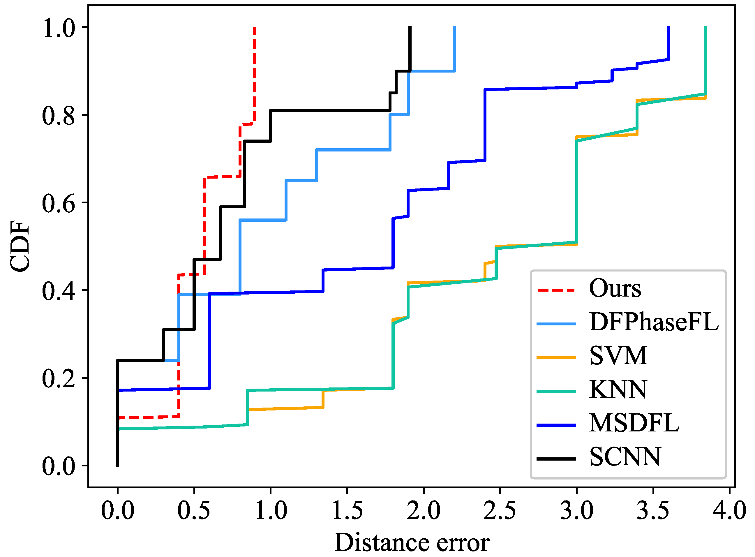
5.7. Comparison with Popular Algorithms

To comprehensively evaluate the performance of the proposed algorithm, we compared it with the currently popular DFPhaseFL, MSDFL [39], and SCNN [40] algorithms and traditional SVM and KNN algorithms with a sample size of 20,000. As shown in

Table 3. Experimental comparison with popular algorithms.

Positioning Algorithm	Cumulative Probability Distribution of Positioning Error/%		Average Positioning Error/m
	Distance Error = 0∼0.4 m	Distance Error = 0∼0.8 m
Ours	43	64	0.67
SCNN	41	59	0.77
DFPhaseFL	37	52	0.83
MSDFL	18	41	1.15
SVM	10	17	2.21
KNN	9	19	2.38

, our proposed algorithm exhibits significant advantages in terms of positioning accuracy. Specifically, the algorithm has a 43% probability of achieving a distance error within 0.4 m and a 64% probability of achieving a distance error within 0.8 m, which are significantly higher than the other four algorithms. Additionally, our algorithm exhibits the smallest average error, reaching 0.67 m. These data provide strong evidence for the excellent performance of the proposed algorithm in terms of positioning accuracy and stability.

Figure 9 illustrates the comparison between various algorithms in terms of their cumulative distribution function and coordinate estimation error. Notably, the proposed method exhibits remarkable positioning accuracy, surpassing both popular positioning systems and traditional machine learning algorithms. Remarkably, 43% of the positioning points achieved an error margin of less than 0.4 m, while 64% of the points fell within an error range of 0.8 m. This exceptional performance highlights the superiority of our proposed method over its peers.

6. Conclusions and Future Work

In this study, we propose an innovative multi-modal indoor positioning method tailored for complex indoor environments. Our method delivers high-precision and highly generalizable indoor positioning by seamlessly integrating coarse-grained image matching and fine-grained feature fusion. The experimental results convincingly demonstrate our method’s significant advantages in positioning accuracy, stability, and scalability compared to the existing techniques. Furthermore, our image-based positioning component eliminates the need for additional equipment as it can be effortlessly conducted using a standard mobile phone camera. This makes our method accessible to all smartphone users, greatly expanding its potential applications. Additionally, our algorithm exhibits excellent scalability and portability. Users can effortlessly upload location data to a fingerprint database for real-time updates or create new image fingerprint databases for indoor environments to facilitate accurate positioning in new settings.

In the future, we aim to delve deeper into applying deep learning techniques in indoor positioning to enhance the accuracy and reliability of our approach. Furthermore, we will focus on dynamic fusion strategies for multi-source information and prioritize user privacy protection to promote the continuous development and utilization of indoor positioning technology.

References

1. Wang, C.; Shi, Z.; Wu, F. Intelligent RFID Indoor Localization System Using a Gaussian Filtering Based Extreme Learning Machine. Symmetry 2017, 9, 30. [Google Scholar] [CrossRef]
2. Kang, J.; Seo, J.; Won, Y. Ephemeral ID Beacon-Based Improved Indoor Positioning System. Symmetry 2018, 10, 622. [Google Scholar] [CrossRef]
3. Chen, W.; Guan, L.; Huang, R.; Zhang, M.; Liu, H.; Hu, Y.; Yin, Y. Sustainable development of animal husbandry in China. Bull. Chin. Acad. Sci. (Chin. Version) 2019, 34, 135–144. [Google Scholar]
4. Yang, Z.; Xue, B. Development history and trend of beidou satellite navigation system. J. Navig. Position. 2022, 10, 1–14. [Google Scholar]
5. Tu, W.; Guo, C. Review of indoor positioning methods based on machine learning. In Proceedings of the 12th China Satellite Navigation Annual Conference, Nanchang, China, 26–28 May 2021; pp. 91–96. [Google Scholar]
6. Lu, H.; Liu, S.; Hwang, S.H. Local Batch Normalization-Aided CNN Model for RSSI-Based Fingerprint Indoor Positioning. Electronics 2025, 14, 1136. [Google Scholar] [CrossRef]
7. Piasco, N.; Sidibé, D.; Demonceaux, C.; Gouet-Brunet, V. A survey on visual-based localization: On the benefit of heterogeneous data. Pattern Recognit. 2018, 74, 90–109. [Google Scholar] [CrossRef]
8. Meng, J.; Zou, J. Fingerprint positioning method of CSI based on PCA-SMO. GNSS World China 2021, 46, 13. [Google Scholar]
9. Zhang, Z.; Lee, M.; Choi, S. Deep-Learning-Based Wi-Fi Indoor Positioning System Using Continuous CSI of Trajectories. Sensors 2021, 21, 5776. [Google Scholar] [CrossRef]
10. Che, R.; Chen, H. Channel State Information Based Indoor Fingerprinting Localization. Sensors 2023, 23, 5830. [Google Scholar] [CrossRef]
11. Dai, P.; Yang, Y.; Wang, M.; Yan, R. Combination of DNN and Improved KNN for indoor location fingerprinting. Wirel. Commun. Mob. Comput. 2019, 2019, 4283857. [Google Scholar] [CrossRef]
12. Tian, G.; Yang, Y.; Wang, S.; Yu, X. CSI indoor positioning based on Kmeans clustering. Appl. Electron. Tech. 2016, 42, 62–64. [Google Scholar]
13. Dang, X.; Ru, C.; Hao, Z. An indoor positioning method based on CSI and SVM regression. Comput. Eng. Sci. 2021, 43, 853–861. [Google Scholar]
14. Rao, X.; Li, Z.; Yang, Y.; Wang, S. DFPhaseFL: A robust device-free passive fingerprinting wireless localization system using CSI phase information. Neural Comput. Appl. 2020, 32, 14909–14927. [Google Scholar] [CrossRef]
15. Ashraf, I.; Zikria, Y.B.; Hur, S. Localizing pedestrians in indoor environments using magnetic field data with term frequency paradigm and deep neural networks. Int. J. Mach. Learn. Cybern. 2021, 12, 3203–3219. [Google Scholar] [CrossRef]
16. Wu, D.; Zhang, D.; Xu, C.; Wang, Y.; Wang, H. WiDir: Walking direction estimation using wireless signals. In Proceedings of the 2016 ACM International Joint Conference on Pervasive and Ubiquitous Computing, Heidelberg Germany, 12–16 September 2016; pp. 351–362. [Google Scholar]
17. Zhang, K.; Tan, B.; Ding, S.; Li, Y.; Li, G. Device-free indoor localization based on sparse coding with nonconvex regularization and adaptive relaxation localization criteria. Int. J. Mach. Learn. Cybern. 2023, 14, 429–443. [Google Scholar] [CrossRef]
18. Zhou, M.; Tang, Y.; Tian, Z. WLAN indoor positioning algorithm based on manifold interpolation database construction. J. Electron. Inf. Technol. 2017, 39, 1826–1834. [Google Scholar]
19. Bai, Y.; Jia, W.; Zhang, H.; Mao, Z.; Sun, M. Landmark-based indoor positioning for visually impaired individuals. In Proceedings of the 2014 12th International Conference on Signal Processing (ICSP), Hangzhou, China, 19–23 October 2014; pp. 678–681. [Google Scholar]
20. Yang, J.; Chen, L.; Liang, W. Monocular vision based robot self-localization. In Proceedings of the 2010 IEEE International Conference on Robotics and Biomimetics, Tianjin, China, 14–18 December 2010; pp. 1189–1193. [Google Scholar]
21. Chen, H.; Yao, M.; Gu, Q. Pothole detection using location-aware convolutional neural networks. Int. J. Mach. Learn. Cybern. 2020, 11, 899–911. [Google Scholar] [CrossRef]
22. Werner, M.; Kessel, M.; Marouane, C. Indoor positioning using smartphone camera. In Proceedings of the 2011 International Conference on Indoor Positioning and Indoor Navigation, Guimaraes, Portugal, 21–23 September 2011. [Google Scholar] [CrossRef]
23. Dryanovski, I.; Valenti, R.; Xiao, J. Fast visual odometry and mapping from RGB-D data. In Proceedings of the 2013 IEEE International Conference on Robotics and Automation, Karlsruhe, Germany, 6–10 May 2013; pp. 2305–2310. [Google Scholar]
24. Zhou, S.; Wu, X.; Qi, Y.; Gong, W. Vision-based localization method for indoor mobile robots based on line detection. J. Huazhong Univ. Sci. Technol. (Nat. Sci. Ed.) 2016, 11, 93–97. [Google Scholar]
25. Buyval, A.; Mustafin, R.; Gavrilenkov, M.; Gabdullin, A.; Shimchik, I. Visual localization for copter based on 3D model of environment with CNN segmentation. In Proceedings of the Information Science and Cloud Computing (ISCC 2017); Guangzhou, China, 16–17 December 2017, pp. 36–41.
26. Wu, Z.; Chen, X.; Wang, J.; Wang, X.; Gan, Y.; Fang, M.; Xu, T. OCR-RTPS: An OCR-based real-time positioning system for the valet parking. Appl. Intell. 2023, 53, 17920–17934. [Google Scholar] [CrossRef]
27. Chen, K.; Huang, Y.; Song, X. Convolutional transformer network: Future pedestrian location in first-person videos using depth map and 3D pose. In Proceedings of the 22nd Asia Simulation Conference, Langkawi, Malaysia, 25–26 October 2023; pp. 44–59. [Google Scholar]
28. Fu, J.; Shi, Y.; Hu, Y.; Ming, Y.; Zou, B. Location optimization of on-campus bicycle-sharing electronic fences. Manag. Syst. Eng. 2023, 2, 11. [Google Scholar] [CrossRef]
29. Tacsyürek, M.; Türkdamar, M.U.; Öztürk, C. DSHFS: A new hybrid approach that detects structures with their spatial location from large volume satellite images using CNN, GeoServer and TileCache. Neural Comput. Appl. 2023, 36, 1237–1259. [Google Scholar] [CrossRef]
30. Keil, J.; Korte, A.; Ratmer, A.; Edler, D.; Dickmann, F. Augmented reality (AR) and spatial cognition: Effects of holographic grids on distance estimation and location memory in a 3D indoor scenario. PFG Photogramm. Remote Sens. Geoinf. Sci. 2020, 88, 165–172. [Google Scholar] [CrossRef]
31. Kumar, S.; Raw, R.S.; Bansal, A. Minimize the routing overhead through 3D cone shaped location-aided routing protocol for FANETs. Int. J. Inf. Technol. 2021, 13, 89–95. [Google Scholar] [CrossRef]
32. Miura, T.; Sako, S. 3D human pose estimation model using location-maps for distorted and disconnected images by a wearable omnidirectional camera. IPSJ Trans. Comput. Vis. Appl. 2020, 12, 4. [Google Scholar] [CrossRef]
33. Shi, W.; Chen, Z.; Zhao, K.; Xi, W.; Qu, Y.; He, H.; Guo, Z.; Ma, Z.; Huang, X.; Wang, P.; et al. 3D target location based on RFID polarization phase model. EURASIP J. Wirel. Commun. Netw. 2022, 2022, 17. [Google Scholar] [CrossRef]
34. Liu, H.; Mei, T.; Li, H.; Luo, J. Vision-based fine-grained location estimation. In Multimodal Location Estimation of Videos and Images; Springer: Cham, Switzerland, 2015; pp. 63–83. [Google Scholar]
35. Ge, Y.; Xiong, Y.; From, P.J. Three-dimensional location methods for the vision system of strawberry-harvesting robots: Development and comparison. Precis. Agric. 2023, 24, 764–782. [Google Scholar] [CrossRef]
36. Zhao, Y.; Xu, J.; Wu, J.; Hao, J.; Qian, H. Enhancing camera-based multi-modal indoor localization with device-free movement measurement using WiFi. IEEE Internet Things J. 2019, 7, 1024–1038. [Google Scholar] [CrossRef]
37. Dong, J.; Xiao, Y.; Noreikis, M.; Ou, Z.; Yl-Jski, A. iMoon: Using smartphones for image-based indoor navigation. In Proceedings of the 13th ACM Conference on Embedded Networked Sensor Systems, Seoul, Republic of Korea, 1–4 November 2015. [Google Scholar]
38. Chang, Y.; Chen, J.; Franklin, T.; Zhang, L.; Ruci, A.; Tang, H.; Zhu, Z. Multimodal information integration for indoor navigation using a smartphone. In Proceedings of the 2020 IEEE 21st International Conference on Information Reuse and Integration for Data Science (IRI), Las Vegas, NV, USA, 11–13 August 2020; pp. 59–66. [Google Scholar]
39. Rao, X.; Li, Z. MSDFL: A robust minimal hardware low-cost device-free WLAN localization system. Neural Comput. Appl. 2019, 31, 9261–9278. [Google Scholar] [CrossRef]
40. Agah, N.; Evans, B.; Meng, X.; Xu, H. A local machine learning approach for fingerprint-based indoor localization. In Proceedings of the SoutheastCon 2023, Orlando, FL, USA, 1–16 April 2023; pp. 240–245. [Google Scholar]
Figure 1. System flowchart. The system flowchart shows the coarse-grained offline positioning stage at the top, the fine-grained offline positioning stage below, and the online positioning stage in the middle (The small figure in the upper right corner of the flowchart: the horizontal axis represents the subcarrier index, ranging from 0 to 30; the vertical axis represents the amplitude, ranging from 12 to 28, with the unit being dB).
Symmetry 17 00597 g001
Figure 2. Image processing in the MobileVIT network.
Symmetry 17 00597 g002
Figure 3. Dataset display, including the collected data for each point, with eight images in each direction.
Symmetry 17 00597 g003
Figure 4. The flowchart of the fusion algorithm. (1) The data are standardized and weighted; (2) the features are multiplied and standardized again; and (3) the features are added to generate the fused features (In the small figure situated in the upper left corner, the horizontal axis denotes the subcarrier index, ranging from 0 to 30, while the vertical axis indicates the amplitude, ranging from 12 to 28, with the unit being dB).
Symmetry 17 00597 g004
Figure 5. Simulation diagram of experimental environment.
Symmetry 17 00597 g005
Figure 6. CDF comparison between Wi-Fi positioning and after feature fusion.
Symmetry 17 00597 g006
Figure 7. CDF plot of experimental comparisons under different sample sizes.
Symmetry 17 00597 g007
Figure 8. CDF plots of experimental comparisons under different antenna conditions: (a) comparison between using individual antennas; (b) comparison between using dual antennas.
Symmetry 17 00597 g008
Figure 9. CDF comparison with popular algorithms.
Symmetry 17 00597 g009