Abstract
Fractional calculus generalizes well-known differentiation and integration to noninteger orders, allowing a more accurate framework for modeling complex dynamical behaviors. The application of fractional-order systems is quite wide in engineering, biology, and physics because they inherently capture the memory effects and long-range dependencies. Out of these, fractional jerk chaotic systems have gained attention regarding their applications in secure communication, signal processing, and control systems. This work develops a comparative analysis of a fractional jerk system that includes constant- and variable-order derivatives to contribute to chaos–stability analysis. Additionally, this study uncovers novel chaotic behaviors, further expanding our understanding of complex dynamical systems. The results yield new insights into using variable-order dynamics to enable chaotic systems to better adapt to real applications.
1. Introduction
Fractional calculus generalizes conventional integer-order differentiation and integration to noninteger orders. Recently, it has received much attention since it can model more complex dynamic behaviors than traditional models. As seen in [1,2,3], fractional-order systems provide a more flexible and realistic approach to modeling physical, biological, and engineering processes, especially those with memory effects and long-range dependence [4,5,6,7,8,9].
The most interesting property among the characteristics of fractional systems is chaotic behavior, which might be used in secure communication, encryption, signal processing, and modeling of biological systems [10,11,12]. Being a third-order dynamical system, the so-called jerk system represents one of the simplest paradigmatic examples in studying chaotic dynamics. In fractional order, it exhibits even richer properties, revealing new insights into nonlinear behavior, bifurcations, and synchronization phenomena.
Fractional-order systems extend classical models by incorporating memory effects and long-range dependencies, making them ideal for describing real-world phenomena in engineering, biology, and physics [13,14,15]. Unlike integer-order models, fractional systems provide greater flexibility and accuracy in capturing complex dynamics, particularly chaotic behavior [16].
The solution to these fractional systems is necessary for understanding their stability, bifurcations, and chaotic properties. Some of the fractional jerk chaotic systems, because of their enhanced dynamical properties, have found emerging applications in secure communication, signal processing, and control systems [17,18,19]. This article identifies their constant and variable-order behaviors, offering fresh perspectives on chaos and stability that enhance practical applications.
The novelty of the paper is the comparative analysis of fractional jerk chaotic systems with constant and variable-order derivatives, giving new insights into how dynamic changes in the fractional order affect chaos and stability and bifurcations. Unlike traditional approaches, this work explores the influence of variable-order dynamics, enhancing our understanding of how evolving memory effects shape chaotic behavior. The paper illustrates, in this direction, the potentials of variable-order systems, therefore extending the contribution of fractional systems in secure communications, encryption, signal processing, and control systems. It allows a new avenue toward modeling real-world complex problems with the presence of long memory effects numerically and via computational validation.
In this study, we simulate and investigate dynamical behavior in the fractional jerk system [20] in the following way:
subject to the following constraints:
where , , and .
The fractional jerk system is particularly powerful for the study of chaotic behavior, since fractional derivatives introduce additional degrees of freedom, which can impact system stability and bifurcation structures. It is applicable in control engineering, wherein synchronization of chaos is crucial in secure communication; mechanical and electrical systems, wherein nonlinear dynamics play a key role in oscillatory behavior; and biomedical signal processing, wherein memory effects are significant while modeling physiological processes. An analysis of the fractional jerk system provides deeper insights into the dynamics between memory and chaos; therefore, it is a valuable tool for applied and theoretical research.
Variable-order derivatives are better at modeling systems with disorders that change over time than constant-order derivatives because they are more flexible and can be tuned. Variable-order derivatives enable us to have an evolving memory effect as a system state or a function of an environmental condition, unlike constant-order derivatives, which assume a uniform memory effect throughout system evolution. With dynamic control of the prior-state effect, this kind of flexibility strengthens system stability, thereby inhibiting chaos. In applications like secure communication and signal processing, the capability enables systems to adjust performance adaptively in different situations and improve responsiveness and robustness. Apart from that, variable-order derivatives can describe real-world phenomena if the order of the nonlocality changes with time, hence being extremely useful in engineering and biological systems that demand large control of chaotic dynamics.
In this paper, we present comparative studies of the chaotic behavior that may arise both for the considered fractional-order variable and constant-order jerk system. Variable-order fractional derivatives represent one of the current developments of a fractal-type property: the order of differentiation might vary dynamically and be dependent either on time or on state in general. With a focus on understanding the changes due to variations that chaos goes through, one seeks in-depth comprehension of how fractional dynamics exert such influence on system stability and predictability.
2. Definitions
Definition 1
([21]). The Liouville–Caputo (LC) derivative with constant order α is given as follows:
Definition 2
([22]). The Liouville–Caputo (LC) fractional derivative of variable-order is given as follows:
where denotes the Gamma function.
3. Algorithms for Fractional Systems with Constant vs. Variable Order
Numerical schemes are generally unavoidable to approximate solutions of nonlinear ordinary and partial differential equations for which no closed-form analytical solution is available. However, fractional differential equations (FDEs) are much more challenging in numerical analysis due to their noninteger order derivatives. The Euler approach, Adams–Bashforth method, Adomian decomposition method, homotopy analysis method, Laplace–Adomian decomposition method, and some polynomial interpolation methods have been used to solve FDEs [23,24,25,26,27]. These are considered in the literature.
In applications where either computational efficiency or stability is more important, simpler methods such as the Euler method and similar methods may be preferred, since their implementations are simpler and they are less computationally demanding. However, where precision is in question and, at the same time, computational resources are available, the more advanced techniques to provide better performance for the approximation of fractional derivatives will be the Lagrange two-step interpolation method [28,29]. These kinds of methods provide a satisfactory trade-off between precision and computational burden, and thus, they are valuable tools in analyzing fractional systems, especially in such domains where a high degree of precision is called for.
This section focuses on approximating solutions in [22,30,31] for models using Caputo fractional operators through efficient numerical techniques. The system is as follows:
where * denotes one of the fractional-order operators under consideration and is the initial state of the system using Definition 2. Consider an equispaced over with step size . Let approximate at .
3.1. Constant Order
By using the numerical method in [31], Equation (5) can be reformulated as follows:
where ; Equation (6) is then:
where ; Equation (6) is then:
The solution of Equation (5) is obtained using Lagrange polynomial interpolation as follows:
The 3D constant-order fractional system with Caputo derivative has solutions given by:
and .
and .
and .
3.2. Variable Order
At , Equation (14) is formulated as follows:
Using the two-step Lagrange polynomial interpolation, we approximate the function over the interval as follows:
We now define the following expressions:
Thus, the solutions for the variable-order system with a Caputo derivative are given by:
and .
and .
and .
4. Numerical Simulation
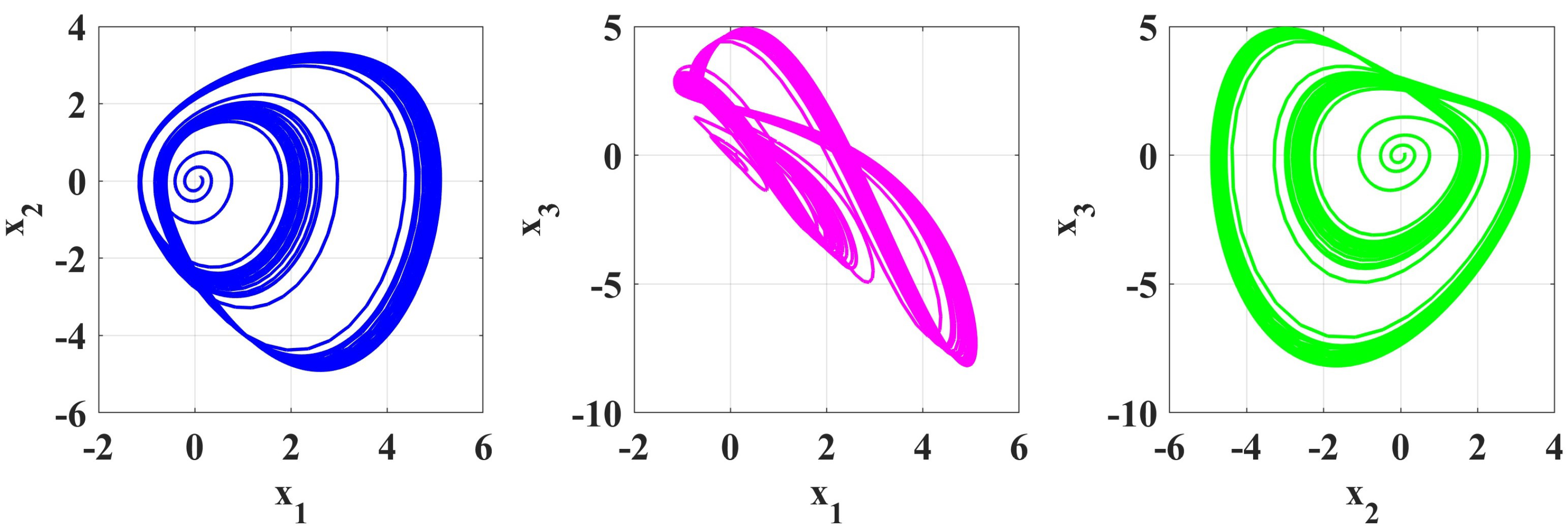
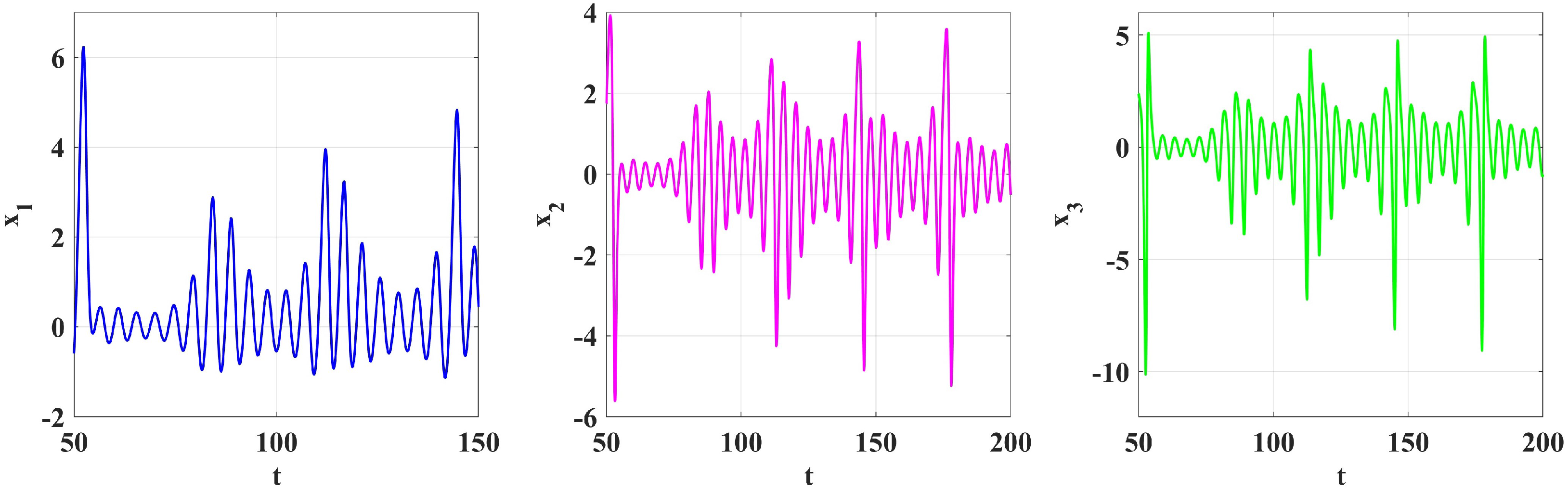
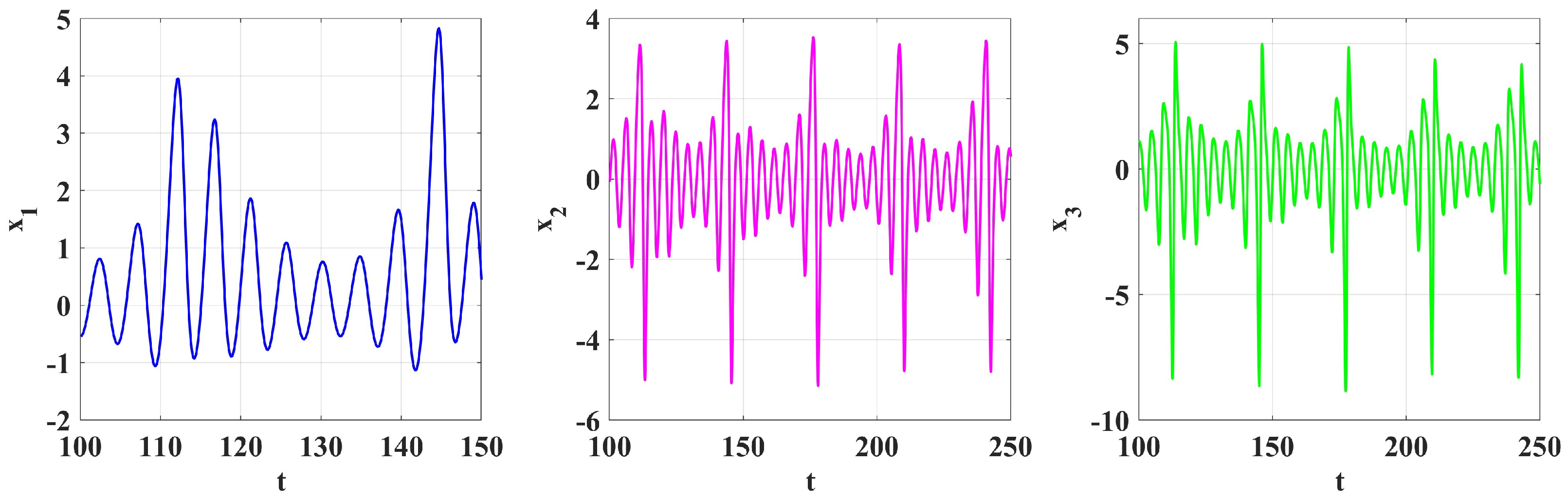
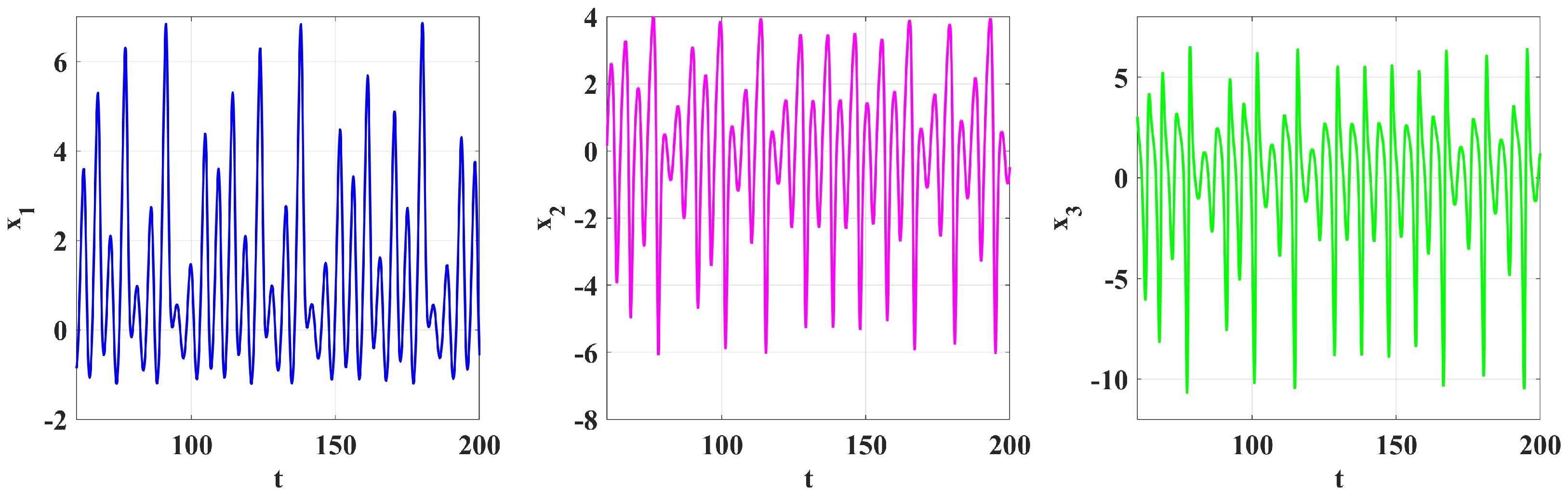
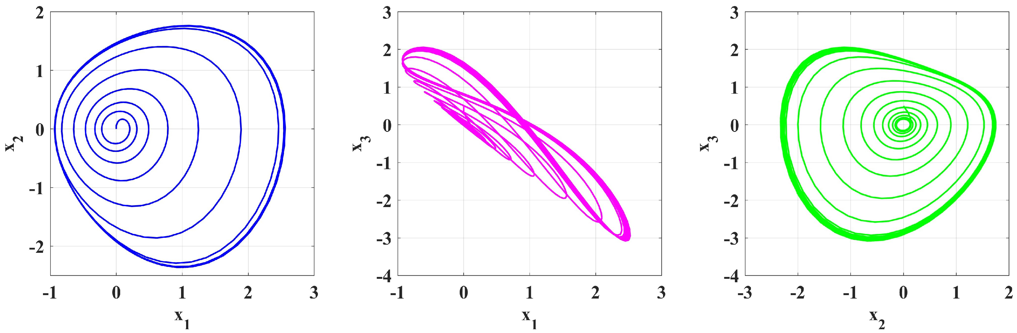
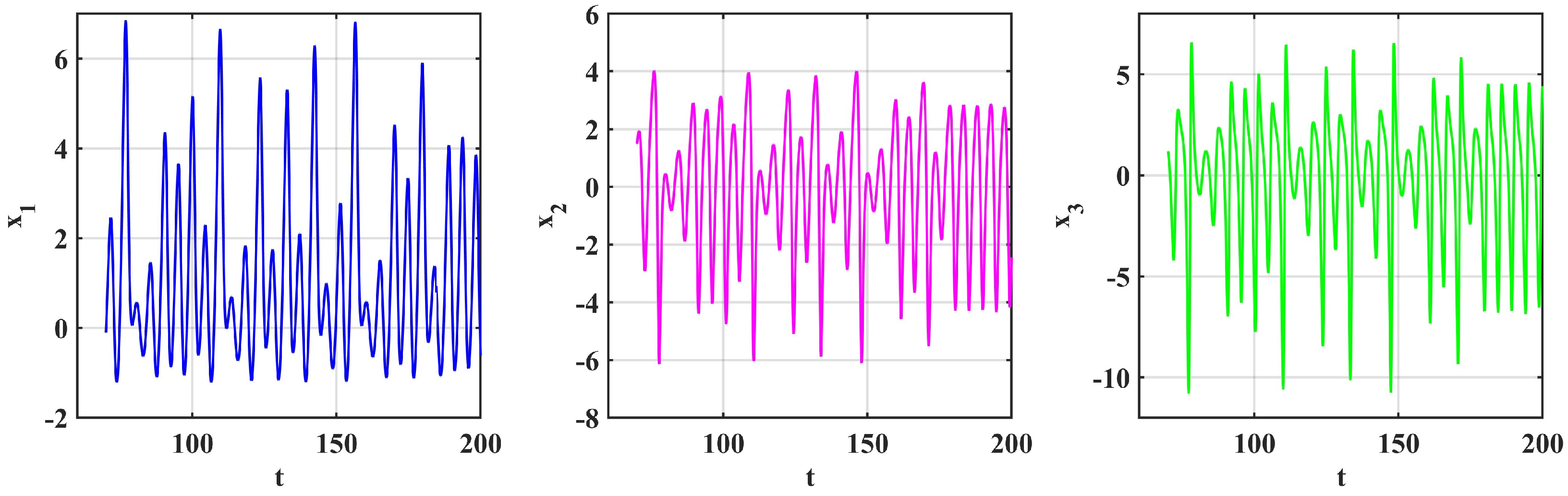
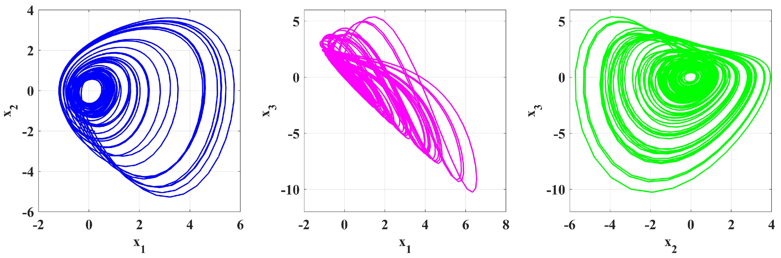
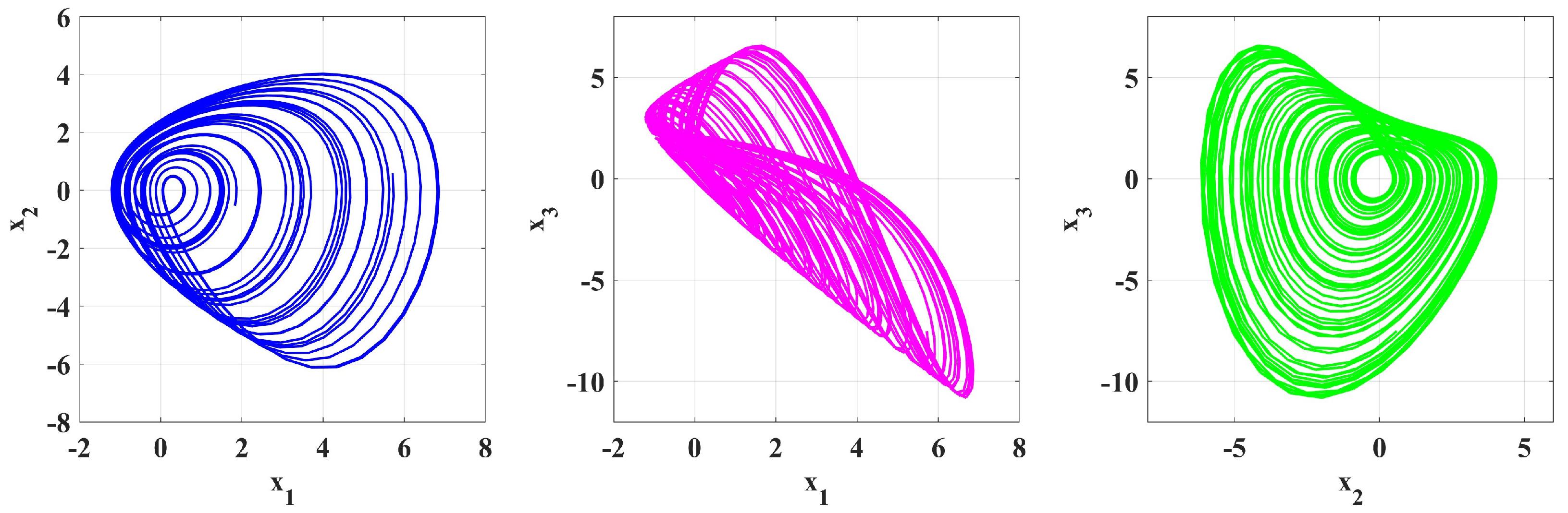
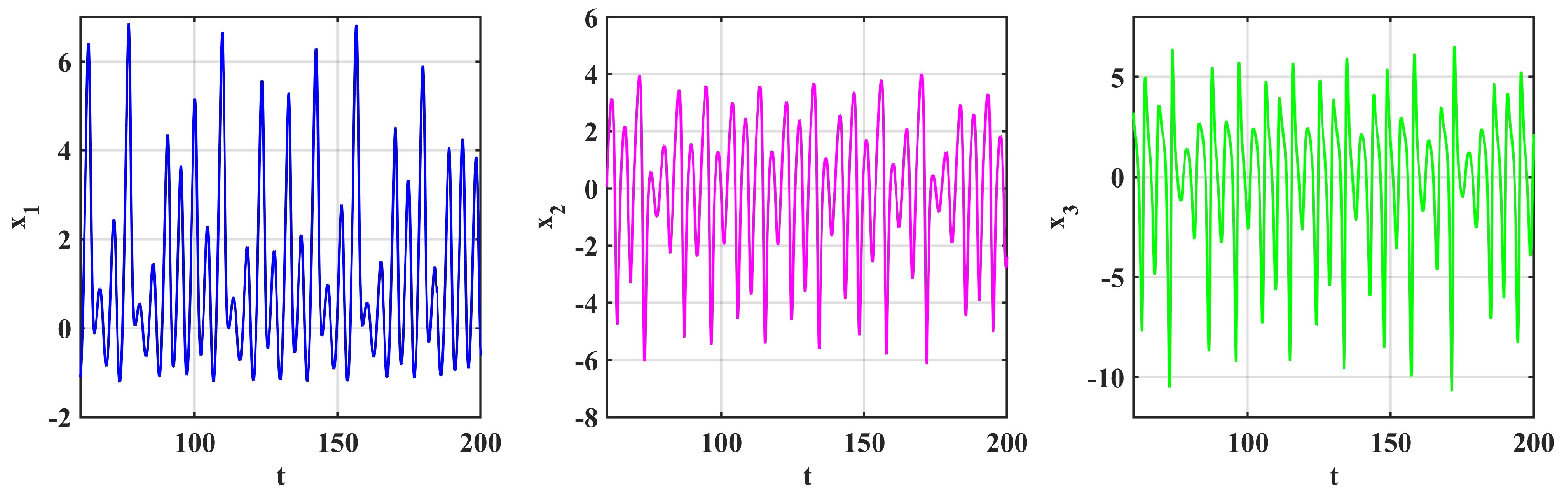
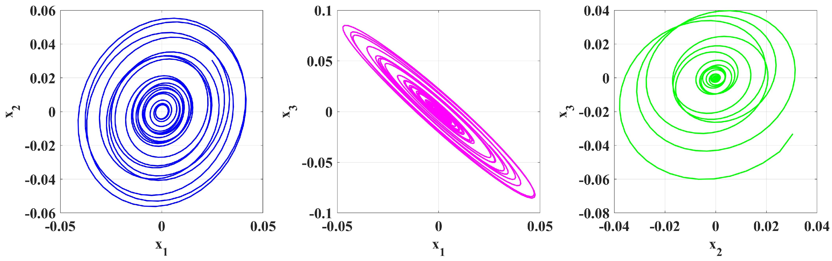
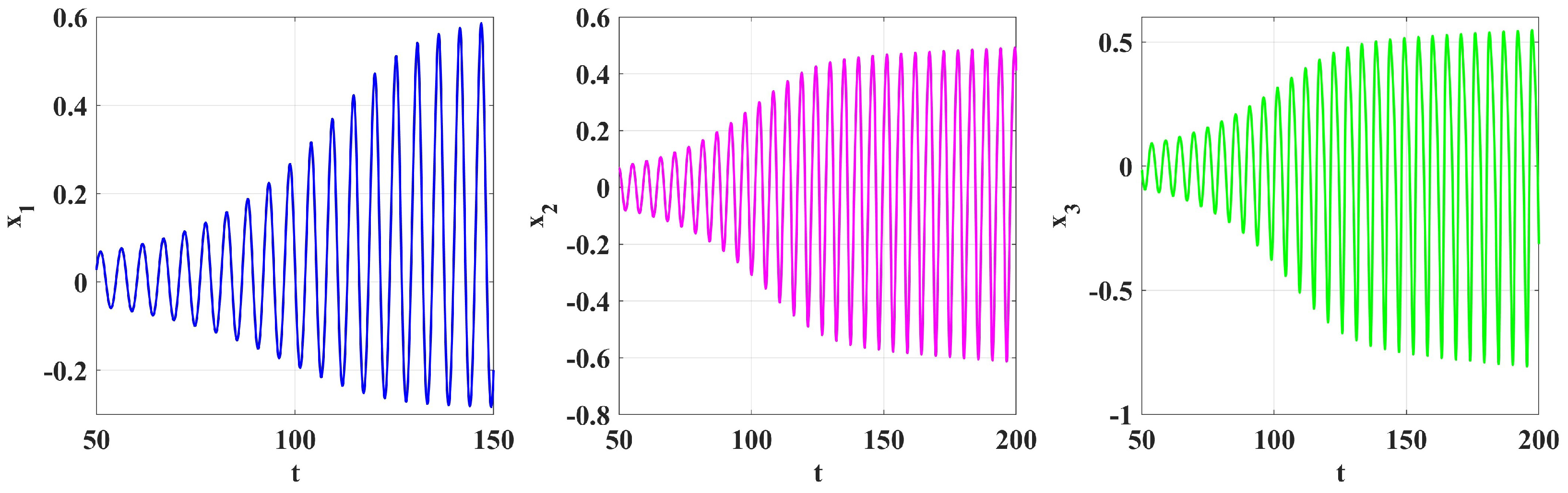
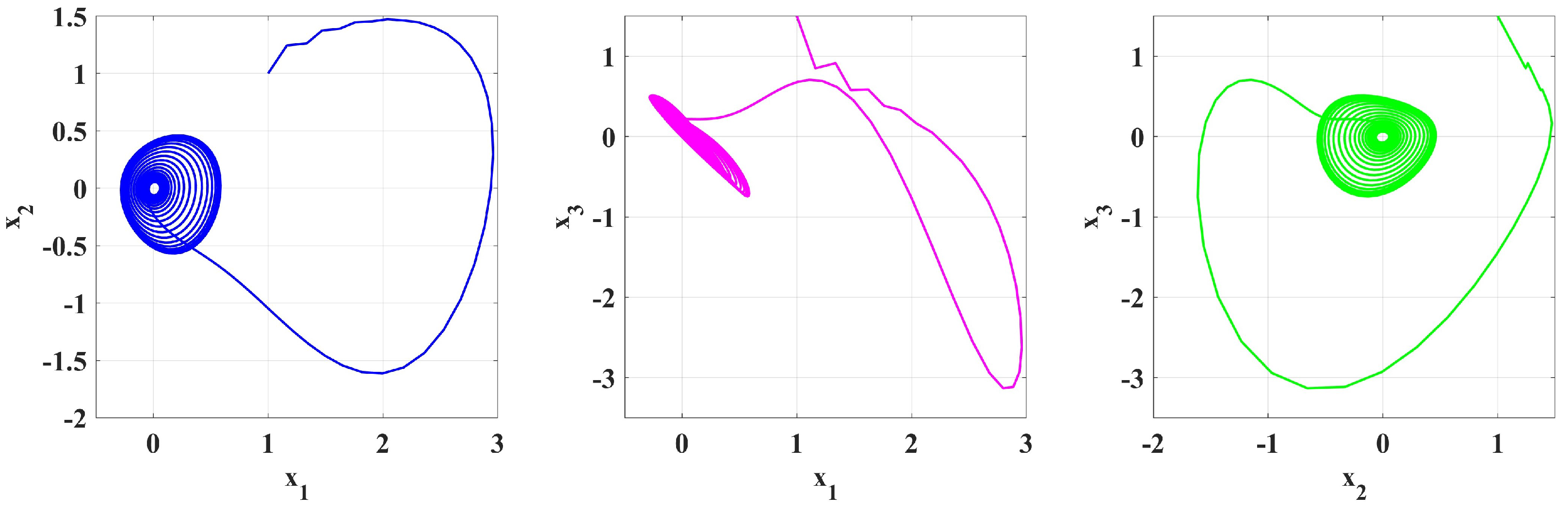
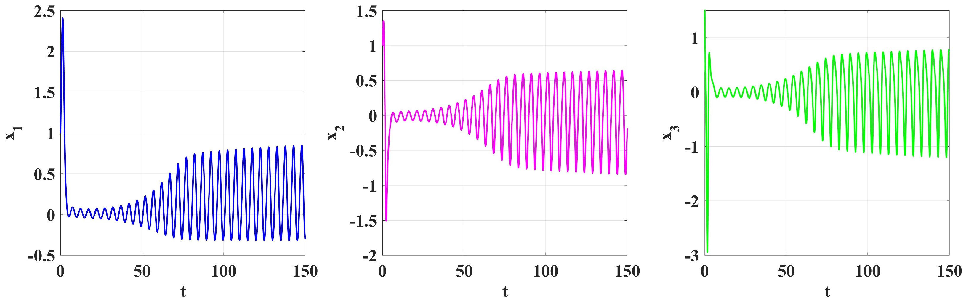
This section explains how system dynamics change with a difference of . The plots in Figure 1, Figure 2, Figure 3, Figure 4, Figure 5, Figure 6, Figure 7, Figure 8, Figure 9, Figure 10, Figure 11 and Figure 12 are the dynamics of a dynamical system for various parameter settings and functional forms of . The phase space plots (first rows) provide the trajectories for different planes (-, -, -), and the time series plots (bottom rows) show the time evolution of the system variables (, , ). Time-varying results in a great deal of chaos and complexity, as seen in Figure 1, Figure 5, and Figure 9 with , , and , respectively. These functional forms create chaotic oscillations and random trajectories, with chaotic behavior dominating for tangent modulation. On the other hand, sustained (e.g., in Figure 2, in Figure 6, and in Figure 10) results in periodic and stable dynamics, characterized by smooth closed orbits in phase space and recurrent oscillations in the time series. Logistic growth Figure 5 displays convergence to stability from chaotic dynamics that asymptotically approaches a constant.
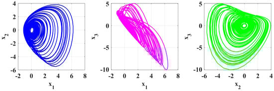
Figure 1.
Dynamic system trajectories for variable-order = 0.95 − 0.05∗(cos(t/5)).

Figure 2.
Dynamic system trajectories for constant-order = 0.98.
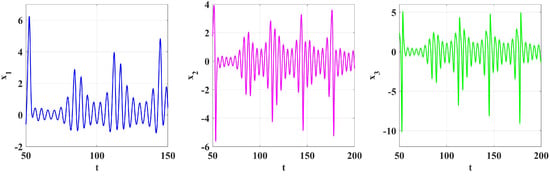
Figure 3.
Time-series analysis for variable-order = 0.95 − 0.05∗(cos(t/5)).
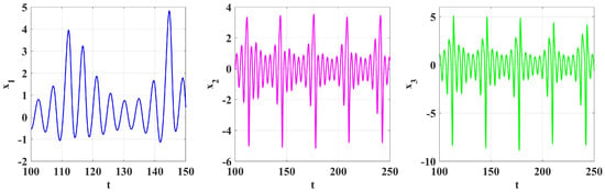
Figure 4.
Time-series analysis for constant-order = 0.98.
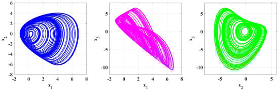
Figure 5.
Dynamic system trajectories for variable-order = 1/(1 + exp()).
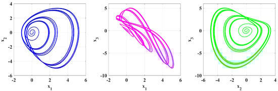
Figure 6.
Dynamic system trajectories for constant-order = 0.95.
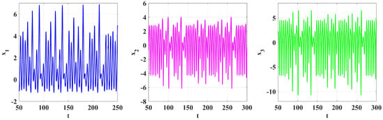
Figure 7.
Time-series analysis for variable-order = 1/(1 + exp()).

Figure 8.
Time-series analysis for constant-order = 0.95.
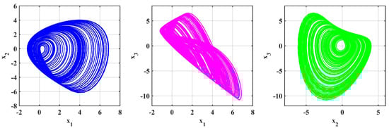
Figure 9.
Dynamic system trajectories for variable-order = tanh(t +1).
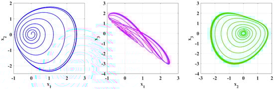
Figure 10.
Dynamic system trajectories for constant-order = 0.99.
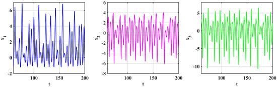
Figure 11.
Time-series analysis for variable-order = tanh(t +1).

Figure 12.
Dynamic system trajectories for constant-order = 0.99.
Figure 13, Figure 14 and Figure 15 show the dynamics for two values of the parameter : a periodic time modulation () and a constant value (). The periodic modulation of time in Figure 13 and Figure 15 generates chaotic dynamics, as confirmed by aperiodic trajectories in phase space with intersecting tracks and oscillating time series with variable amplitude and frequency. The quasiperiodicity of the cosine term brings in complexity, resulting in aperiodic dynamics. The periodic and stable dynamics are shown in Figure 14 and Figure 16, with fixed. The phase space orbits are smooth, closed loops that exhibit a stable limit cycle, and the time series plots exhibit regular oscillations with constant frequencies and amplitudes. This analogy captures the sensitivity of the system to the functional form , in which time-dependent modulation induces chaos and a constant value stabilizes the system, with implications for control in dynamical systems.
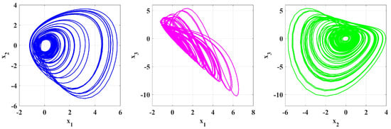
Figure 13.
Dynamic system trajectories for constant-order = 0.96 − 0.03(cos(t/5)).
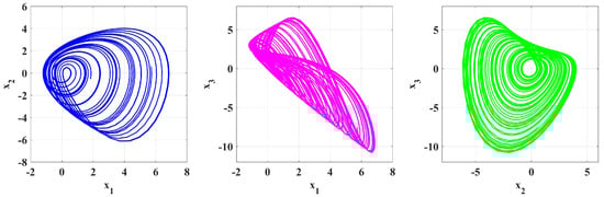
Figure 14.
Dynamic system trajectories for constant-order = 0.96.

Figure 15.
Time-series analysis for constant-order = 0.96 − 0.03(cos(t/5)).
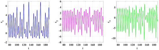
Figure 16.
Time-series analysis for constant-order .
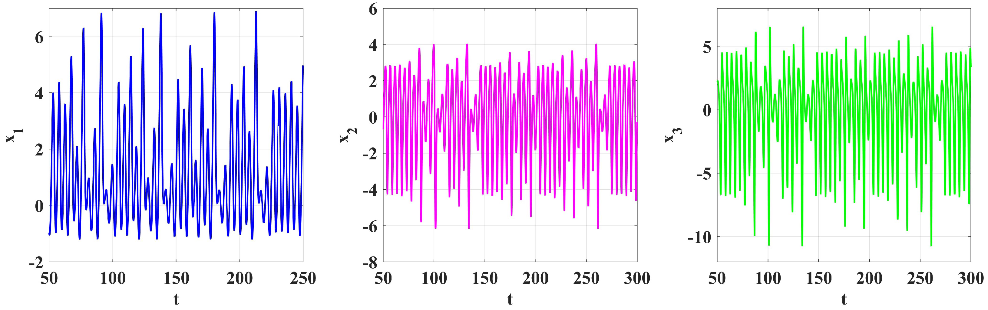
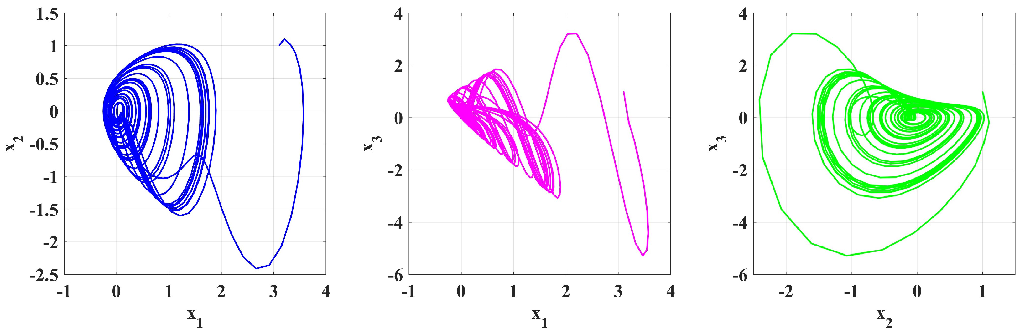
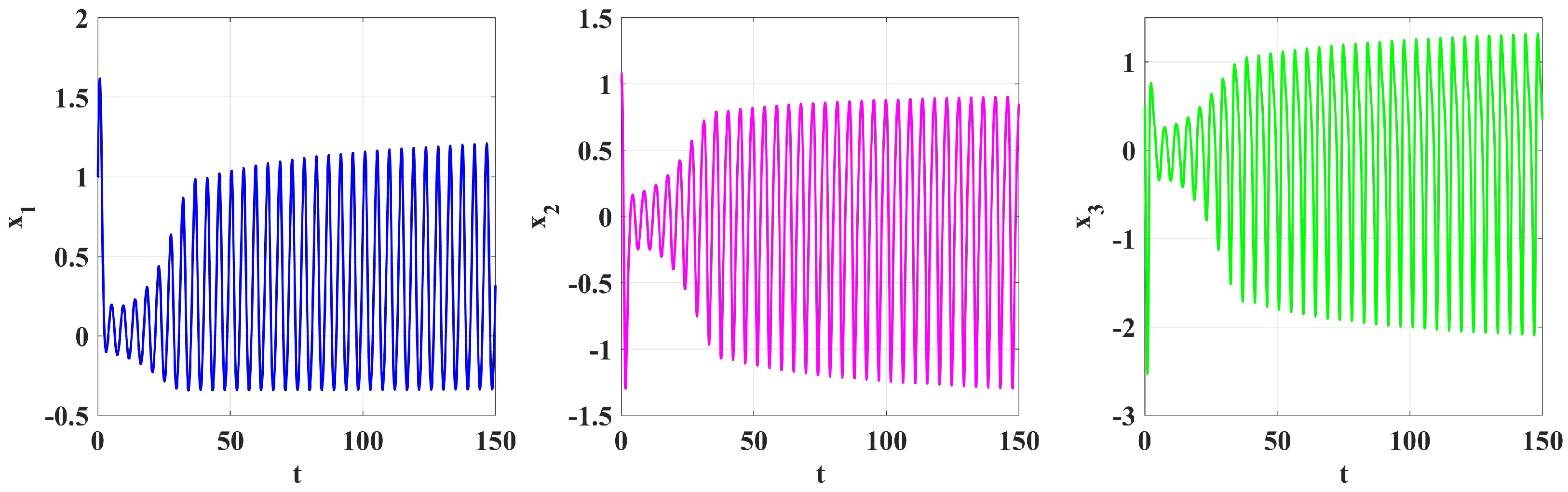
Figure 16, Figure 17, Figure 18, Figure 19, Figure 20, Figure 21 and Figure 22 exhibit novel chaotic and dynamic patterns in a time-varying parameter-dependent system, , , and . Parameterizations add nonlinearity and time modulation and lead to complex phase portraits and oscillatory time-series patterns. The phase-space chaotic attractors have complex shapes and densities, which represent sensitivity to the initial conditions and parameter variations. The time series plots also determine transitions from chaotic to periodic behavior, with the oscillations increasing or stabilizing with time. This task is particularly novel, as it combines nonlinear dynamics with time-varying parameters and offers insight into complex systems like biological rhythms or climate models. The dynamics that arise between periodicity and chaos emphasize the system’s rich and unstable dynamics.
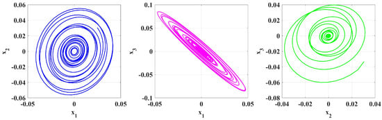
Figure 17.
Dynamic system trajectories for variable-order = 0.90 − 0.05(sin(t/7)).
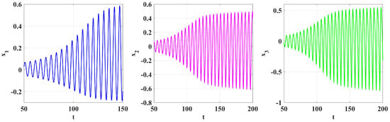
Figure 18.
Time-series analysis for variable-order = 0.90 − 0.05(sin(t/7)).
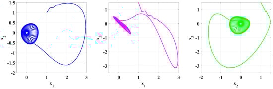
Figure 19.
Dynamic system trajectories for variable-order .
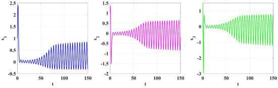
Figure 20.
Time-series analysis for variable-order .
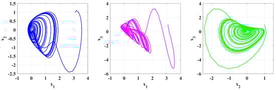
Figure 21.
Dynamic system trajectories variable-order = tanh(t +1).
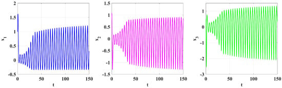
Figure 22.
Time-series analysis for variable-order tan.
The results suggest that time-dependent fractional orders () introduce chaos and complexity, while the constant stabilizes with a periodic output. Chaotic behavior of modulated creates unpredictable, aperiodic paths, whereas constant yield smooth, closed orbits. Periodic-chaotic transitions are a demonstration of the system’s sensitivity to fractional parameters, and they indicate its application in simulating biological rhythms, climate phenomena, and secure communication. Chaotic behavior has to be understood to develop complex systems in the real world because chaos can be engineered to create engineering, cryptography, and nonlinear control systems.
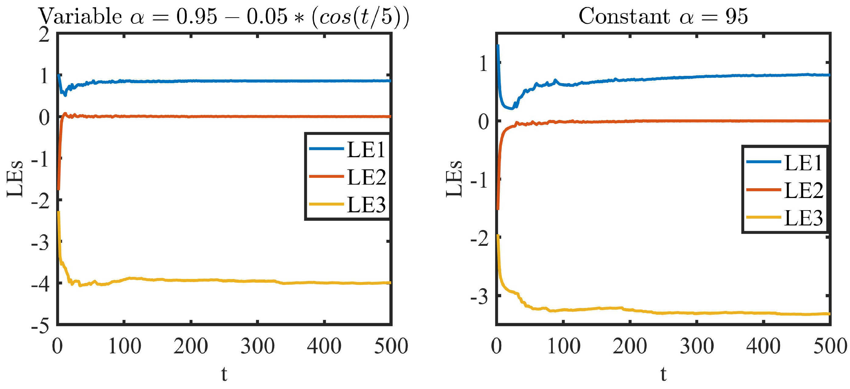
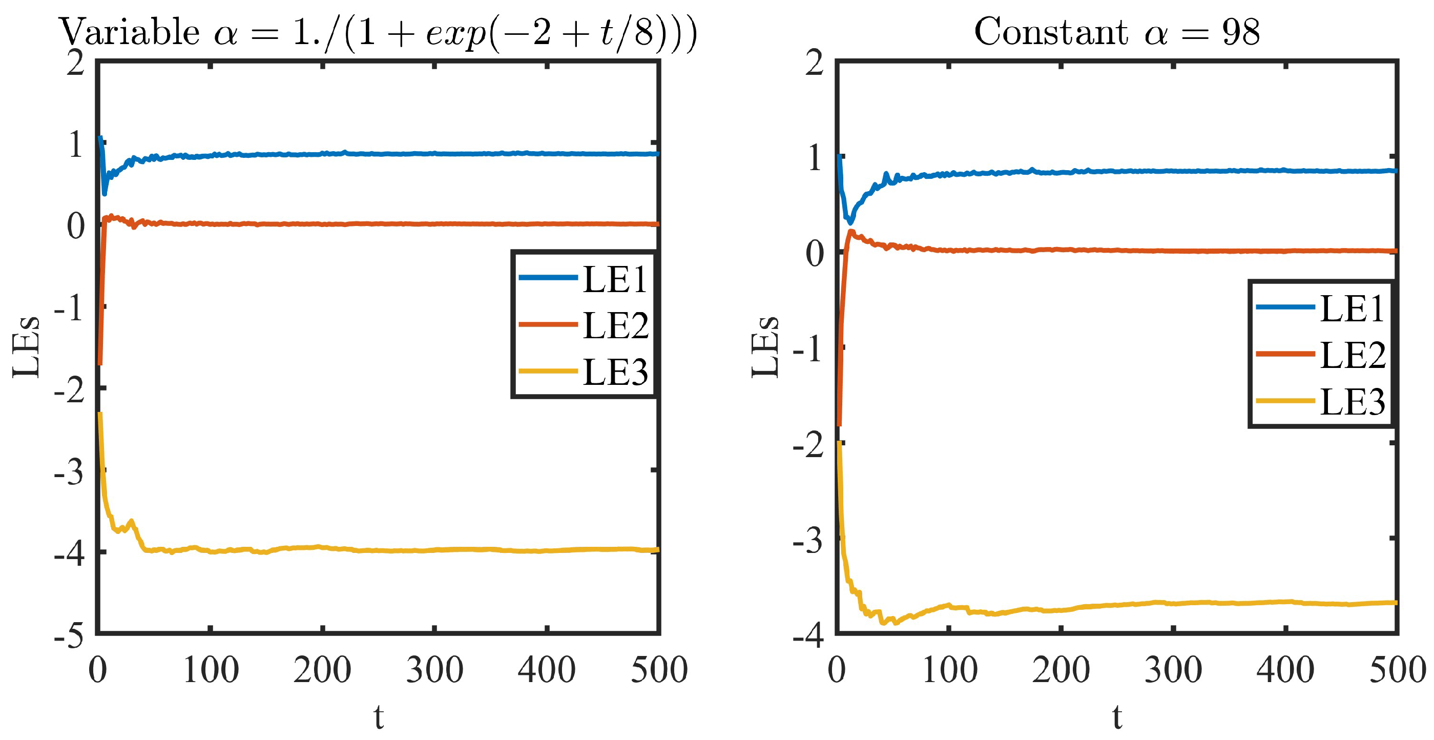
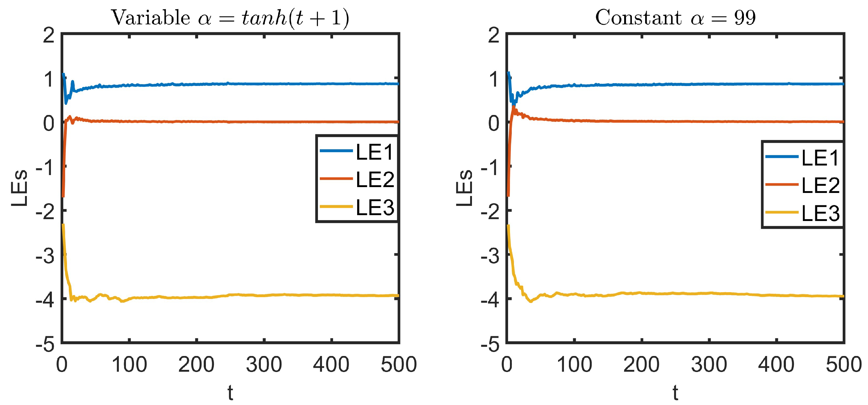
The time evolution of Lyapunov exponents (LE1, LE2, LE3) of variable and constant fractional orders is presented in Figure 23, Figure 24 and Figure 25. Variable fractional orders, in all three cases, exhibit more intense transient behaviors compared to their constant counterparts because they are time-varying. In Figure 23, gives periodic oscillations, with LE1 settling at close to , LE2 at 0, and LE3 at approximately . Similarly, in Figure 24, with , LE1 settles just above , with continuing chaos, while LE2 and LE3 settle at 0 and , respectively. Figure 25, with , illustrates the same stabilization, as LE1 is chaotic, LE2 has quasiperiodic behavior, and LE3 shows contraction in some dimensions of the attractor. In all the figures, the fractional orders that are fixed stabilize faster than variable ones, but the asymptotic behavior is the same. LE1 is positive in both cases and indicates chaotic dynamics, LE2 approaches 0, and LE3 approaches a negative value, indicating state-space contraction. Variable orders (oscillatory cosine, exponential sigmoid, and hyperbolic tangent) affect the transient behavior but ultimately approach behavior similar to the constant fractional order systems. These results demonstrate the equivalence of fractional-order variability with system stability and introduce knowledge on how chaos or stability can be regulated in dynamical systems.
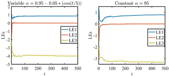
Figure 23.
Evolution of Lyapunov exponents for variable and constant fractional order.

Figure 24.
Evolution of Lyapunov exponents for variable and constant fractional order.
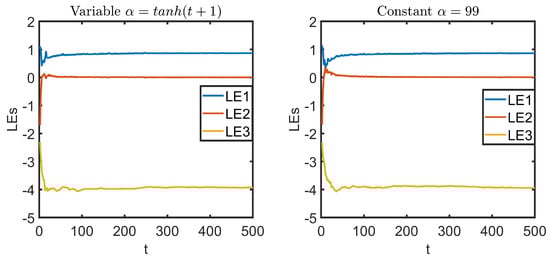
Figure 25.
Evolution of Lyapunov exponents for variable and constant fractional order.
5. Numerical Solutions
This section presents a comparative study of a system using constant and variable fractional orders. This investigation analyzes the system response under varying definitions to consider the impact of memory effects on the temporal development of variables. This study explores the interaction between constant-order (C) and variable-order (V) elements using numerical simulations, underscoring the significance of time-dependent fractional dynamics in characterizing the behavior, stability, and complexity of systems.
Table 1 and Table 2 show how a system with two different values of changes over time. They show how the constant-order components (C) and variable-order components (V) interact with three variables (). In the first example (), the system creates smooth periodic modulations, and the components C and V evolve gradually, for instance, the monotonous increase of and and the reduction of and . In contrast, the second example () is characterized by more intricate nonlinear dynamics, with an aperiodic oscillation of V, especially for and , characteristic of chaotic behavior. Constant-order components (C) show smoother dynamics, while variable-order components (V) show transient and chaotic dynamics.

Table 1.
Comparison of C and V for and .
Table 2.
Comparison of C and V for , .
The comparison between C and V for and is presented in Table 3. The values show a high degree of agreement in all state variables and . Although slight differences appear at certain time steps, the overall consistency supports the validity of the variable-order model.
Table 3.
Comparison of C and V for , .
The system is sensitive to the time-dependent fractional order , with sinusoidal fluctuations causing periodic behavior and sigmoid functions causing chaotic dynamics. Variable-order derivatives are implemented using a discretized Caputo technique, updating at each step, and using quadrature techniques and adaptive time-stepping ensures precision, even when varies quickly.
6. Conclusions
This paper extends fractional calculus through the systematic comparison of constant- and variable-order derivatives in jerk systems, exhibiting their unique capacity to model real-world phenomena with memory effects and nonlocal interactions. Through numerical simulations, we unveil previously unknown chaotic regimes, which appear uniquely in variable-order systems with dynamic multistability transitions. Our results bring us to the conclusion that a changing order produces chaotic and irregular dynamics, with unpredictable trajectories and nonperiodic oscillations. The steady and periodic behavior is the result of constant order. How the system produces constant and smooth oscillations and closed orbits is characteristic of regular and predictable dynamics. The relevance of fractional dynamics in the description and management of intricate events is brought to the fore by this. While variable order leads to more severe transients, it finally settles down to behave like constant orders in the long term. LE1 has a positive value, showing chaos, but LE2 and LE3 show neutral and contracting dynamics, respectively. This shows how the variable order has an effect on the final system stability, but does not change it. In future work, we plan to explore new fractional models, as discussed in [32,33,34], and comparative analysis with other numerical methods in [35,36,37].
Author Contributions
R.A. and N.A.A.; Conceptualization, investigation, writing—original draft, methodology. M.A.A. and R.D.A.; Formal analysis, investigation, writing—review and editing. All authors have read and agreed to the published version of the manuscript.
Funding
This research received no external funding.
Data Availability Statement
The original contributions presented in the study are included in the article, further inquiries can be directed to the corresponding author.
Conflicts of Interest
The authors declare no conflicts of interest.
References
- Dalir, M.; Bashour, M. Applications of fractional calculus. Appl. Math. Sci. 2010, 4, 1021–1032. [Google Scholar]
- Sun, H.; Zhang, Y.; Baleanu, D.; Chen, W.; Chen, Y. A new collection of real world applications of fractional calculus in science and engineering. Commun. Nonlinear Sci. Numer. Simul. 2018, 64, 213–231. [Google Scholar] [CrossRef]
- Machado, J.A.T.; Silva, M.F.; Barbosa, R.S.; Jesus, I.S.; Reis, C.M.; Marcos, M.G.; Galhano, A.F. Some applications of fractional calculus in engineering. Math. Probl. Eng. 2010, 2010, 639801. [Google Scholar] [CrossRef]
- Hasan, F.L.; Abdoon, M.A.; Saadeh, R.; Qazza, A.; Almutairi, D.K. Exploring analytical results for (2 + 1) dimensional breaking soliton equation and stochastic fractional Broer-Kaup system. AIMS Math. 2024, 9, 11622–11643. [Google Scholar] [CrossRef]
- Gumaa, F.E.L.; Abdoon, M.A.; Qazza, A.; Saadeh, R.; Arishi, M.A.; Degoot, A.M. Analyzing the impact of control strategies on Visceral Leishmaniasis: A mathematical modeling perspective. Eur. J. Pure Appl. Math. 2024, 17, 1213–1227. [Google Scholar] [CrossRef]
- Alsubaie, N.E.; Gumaa, F.E.L.; Boulehmi, K.; Al-Kuleab, N.; Abdoon, M.A. Improving influenza epidemiological models under Caputo fractional-order calculus. Symmetry 2024, 16, 929. [Google Scholar] [CrossRef]
- Liu, T.; Yin, X.; Liu, Q.; Hounye, A.H. Modeling SARS coronavirus-2 omicron variant dynamic via novel fractional derivatives with immunization and memory trace effects. Alex. Eng. J. 2024, 86, 174–193. [Google Scholar] [CrossRef]
- Oprzędkiewicz, K.; Rosół, M.; Mitkowski, W. Modeling of thermal traces using fractional order, a discrete, memory-efficient model. Energies 2022, 15, 2257. [Google Scholar] [CrossRef]
- Allagui, A.; Zhang, D.; Khakpour, I.; Elwakil, A.S.; Wang, C. Quantification of memory in fractional-order capacitors. J. Phys. D Appl. Phys. 2019, 53, 02LT03. [Google Scholar] [CrossRef]
- Rahman, Z.-A.S.; Jasim, B.H.; Al-Yasir, Y.I.A.; Hu, Y.-F.; Abd-Alhameed, R.A.; Alhasnawi, B.N. A new fractional-order chaotic system with its analysis, synchronization, and circuit realization for secure communication applications. Mathematics 2021, 9, 2593. [Google Scholar] [CrossRef]
- Karaca, Y.; Baleanu, D. Advanced fractional mathematics, fractional calculus, algorithms and artificial intelligence with applications in complex chaotic systems. Chaos Theory Appl. 2023, 5, 257–266. [Google Scholar]
- Karaca, Y.; Baleanu, D.; Zhang, Y.-D.; Gervasi, O.; Moonis, M. Multi-Chaos, Fractal and Multi-Fractional Artificial Intelligence of Different Complex Systems; Academic Press: Cambridge, MA, USA, 2022. [Google Scholar]
- Zhang, J.-X.; Zhang, X.; Boutat, D.; Liu, D.-Y. Fractional-Order Complex Systems: Advanced Control, Intelligent Estimation and Reinforcement Learning Image-Processing Algorithms. Fractal Fract. 2025, 9, 67. [Google Scholar] [CrossRef]
- Yang, F.; Mou, J.; Liu, J.; Ma, C.; Yan, H. Characteristic analysis of the fractional-order hyperchaotic complex system and its image encryption application. Signal Process. 2020, 169, 107373. [Google Scholar] [CrossRef]
- Dhakshinamoorthy, V.; Wu, G.-C.; Banerjee, S. Chaotic Dynamics of Fractional Discrete Time Systems; CRC Press: Boca Raton, FL, USA, 2024. Comput. Methods Programs Biomed. 2024, 254, 108306. [Google Scholar]
- Karaca, Y. Multi-chaos, fractal and multi-fractional AI in different complex systems. In Multi-Chaos, Fractal and Multi-Fractional Artificial Intelligence of Different Complex Systems; Elsevier: Amsterdam, The Netherlands, 2022; pp. 21–54. [Google Scholar]
- Naik, P.A.; Yavuz, M.; Qureshi, S.; Owolabi, K.M.; Soomro, A.; Ganie, A.H. Memory impacts in hepatitis C: A global analysis of a fractional-order model with an effective treatment. Comput. Methods Programs Biomed. 2024, 254, 108306. [Google Scholar] [CrossRef]
- Vaidyanathan, S.; Akgul, A.; Kacar, S. A new chaotic jerk system with two quadratic nonlinearities and its applications to electronic circuit implementation and image encryption. Int. J. Comput. Appl. Technol. 2018, 58, 89–101. [Google Scholar] [CrossRef]
- Khan, N.A.; Hameed, T.; Qureshi, M.A.; Akbar, S.; Alzahrani, A.K. Emulate the chaotic flows of fractional jerk system to scramble the sound and image memo with circuit execution. Phys. Scr. 2020, 95, 065217. [Google Scholar] [CrossRef]
- Wang, Q.; Sang, H.; Wang, P.; Yu, X.; Yang, Z. A novel 4D chaotic system coupling with dual-memristors and application in image encryption. Sci. Rep. 2024, 14, 29615. [Google Scholar] [CrossRef]
- Oldham, K.B.; Spanier, J. The Fractional Calculus: Theory and Applications of Differentiation and Integration to Arbitrary Order; Academic Press: New York, NY, USA, 1974; p. 9780125255509. [Google Scholar]
- Solís-Pérez, J.E.; Gómez-Aguilar, J.F.; Atangana, A. Novel numerical method for solving variable-order fractional differential equations with power, exponential and Mittag–Leffler laws. Chaos Solitons Fractals 2018, 114, 175–185. [Google Scholar] [CrossRef]
- Pu, Y.-F. Fractional-order Euler–Lagrange equation for fractional-order variational method: A necessary condition for fractional-order fixed boundary optimization problems in signal processing and image processing. IEEE Access 2016, 4, 10110–10135. [Google Scholar] [CrossRef]
- Ali, Z.; Rabiei, F.; Hosseini, K. Fractal-Fractional Third-Order Adams-Bashforth Method. SSRN Electron. J. 2022. [Google Scholar] [CrossRef]
- Bildik, N. Implementation to the Different Differential Equations of Homotopy Analysis, Differential Transformed and Adomian Decomposition Method. Int. J. Model. Optim. 2013, 3, 529–534. [Google Scholar] [CrossRef]
- Kshirsagar, K.; Nikam, V.; Gaikwad, S.; Tarate, S. Fuzzy Laplace-Adomian Decomposition method for solving Fuzzy Klein-Gordan equations. Authorea Inc. Aug. 2022. [Google Scholar] [CrossRef]
- Zhang, X.; Guo, X.; Xu, A. Computations of Fractional Differentiation by Lagrange Interpolation Polynomial and Chebyshev Polynomial. Inf. Technol. J. 2012, 11, 557–559. [Google Scholar] [CrossRef]
- Buhader, A.A.; Abbas, M.; Imran, M.; Omame, A. Comparative analysis of a fractional co-infection model using nonstandard finite difference and two-step Lagrange polynomial methods. Partial Differ. Equ. Appl. Math. 2024, 10, 100702. [Google Scholar] [CrossRef]
- Ramalakshmi, K.; Sundaravadivoo, B. Necessary conditions for Ψ-Hilfer fractional optimal control problems and Ψ-Hilfer two-step Lagrange interpolation polynomial. Int. J. Dyn. Control 2024, 12, 42–55. [Google Scholar] [CrossRef]
- Alqahtani, A.M.; Chaudhary, A.; Dubey, R.S.; Sharma, S. Comparative analysis of the chaotic behavior of a five-dimensional fractional hyperchaotic system with constant and variable order. Fractal Fract. 2024, 8, 421. [Google Scholar] [CrossRef]
- Butt, A.I.K.; Ahmad, W.; Rafiq, M.; Baleanu, D. Numerical analysis of Atangana-Baleanu fractional model to understand the propagation of a novel corona virus pandemic. Alex. Eng. J. 2022, 61, 7007–7027. [Google Scholar] [CrossRef]
- Metsebo, J.; Abdou, B.; Ngatcha, D.T.; Ngongiah, I.K.; Kuate PD, K.; Pone JR, M. Analysis of a resistive-capacitive shunted Josephson junction with a topologically nontrivial barrier coupled to an RLC resonator. Chaos Fractals 2024, 1, 31–37. [Google Scholar]
- Bucio, A.; Tututi-Hernández, E.S.; Uriostegui-Legorreta, U. Analysis of the dynamics of a ϕ6 Duffing-type jerk system. Chaos Theory Appl. 2024, 6, 83–89. [Google Scholar] [CrossRef]
- Khan, A.; Li, C.; Zhang, X.; Cen, X. A two-memristor-based chaotic system with symmetric bifurcation and multistability. Chaos Fractals 2025, 2, 1–7. [Google Scholar] [CrossRef]
- Uddin, M.J.; Santra, P.K.; Rana SM, S.; Mahapatra, G. Chaotic dynamics of the fractional-order predator-prey model incorporating Gompertz growth on prey with Ivlev functional response. Chaos Theory Appl. 2024, 6, 192–204. [Google Scholar] [CrossRef]
- Berir, M. The impact of white noise on chaotic behavior in a financial fractional system with constant and variable order: A comparative study. Eur. J. Pure Appl. Math. 2024, 17, 3915–3931. [Google Scholar] [CrossRef]
- Saadeh, R.; Alshawabkeh, A.; Khalil, R.; Abdoon, M.A.; Taha, N.; Almutairi, D.K. The Mohanad transforms and their applications for solving systems of differential equations. Eur. J. Pure Appl. Math. 2024, 17, 385–409. [Google Scholar] [CrossRef]


Disclaimer/Publisher’s Note: The statements, opinions and data contained in all publications are solely those of the individual author(s) and contributor(s) and not of MDPI and/or the editor(s). MDPI and/or the editor(s) disclaim responsibility for any injury to people or property resulting from any ideas, methods, instructions or products referred to in the content. |
© 2025 by the authors. Licensee MDPI, Basel, Switzerland. This article is an open access article distributed under the terms and conditions of the Creative Commons Attribution (CC BY) license (https://creativecommons.org/licenses/by/4.0/).