Abstract
The increasing penetration of renewable generations (RGs) poses significant challenges to the operation of transmission power systems, especially for not only steady-stage uncertainties but also dynamic-state stability. Hence, the symmetry of RGs and synchronous generations (SGs) should be improved by a proper planning strategy. For this purpose, a multi-stage stochastic planning method is proposed for transmission power systems (TPSs) considering dynamic frequency stability. Specifically, the progressive uncertainties of RGs over stages are addressed with a multi-stage stochastic method with nonanticipativity constraints. In this scheme, the uncertainty is represented by probability-weighted scenarios, and the planning decisions are only dependent on current realizations of RG uncertainties according to nonanticipativity constraints to improve planning efficiency. Moreover, the dynamic frequency stability constraints are derived considering the frequency regulation strategy of RGs, and these nonconvex constraints are further linearized with high accuracy by a maximal affine function-based method to improve the compatibility with the planning model. Subsequently, a progressive hedging algorithm (PHA) is designed to reduce the computational burden by decomposing the multi-scenario high-dimensional model into multiple small-scale models. Finally, the effectiveness of the proposed method, as well as its superiority over existing approaches, are validated through numerical experiments.
1. Introduction
The symmetry of RGs and SGs plays an essential role in the stable operation of modern power systems. However, the symmetry is significantly threatened by the increase in the penetration RGs. In this case, a multi-stage stochastic planning method considering dynamic frequency stability is proposed to improve the system symmetry. In this section, the motivation of this paper is introduced, including background and challenges, State-of-the-Art review and research gaps, as well as primary focus and contributions.
1.1. Background and Challenge
For traditional power system planning, power sources and transmission lines are sitting and sizing to increase load supplies. However, the rapid increase in the penetration of RGs poses significant challenges to the secure and stable operation of modern TPSs. Specifically:
Challenge 1: From aspects of the steady-state scale, the randomness and fluctuation in RG outputs threaten the real-time power balance of TPSs, leading to more power reserve from synchronous generators and adjustable loads to address the uncertainty [1].
Challenge 2: For the dynamic-state scale, RGs are generally interfaced with the grid through power converters, which isolate the rotational speed of wind turbines (WTs) from the system’s frequency. Hence, the inverter-based RGs cannot inherently release the kinetic energy stored in their rotating masses like SGs during frequency events [2].
These steady- and dynamic-state challenges serve as significant issues for modern TPSs, especially for the TPSs with improper proportions of RGs, although some valuable scheduling and frequency regulation strategies have been employed [1,2]. Hence, for modern TPS planning, these challenges urgently need to be addressed by improving the symmetry of RGs and SGs with strong reserve and frequency capacities in the planning strategy.
1.2. State-of-the-Art Review
Some research has been conducted for TPS planning with the consideration of RG uncertainties, generally with a two-stage method that the first stage determines the planning decisions, and the second stage evaluates the planning strategy with operational scenarios, such as the two-stage robust method and the two-stage stochastic method [3]. The two-stage robust method determines the planning strategy with the guidance of the worst realization of uncertainties. A two-stage distributionally robust optimization model was proposed in [4] for the transmission network expansion planning, where the minimum expectation of the renewable utilization probability was maximized among a set of certain probability distributions within an ambiguity set. In [5], a two-stage robust transmission network expansion planning model was presented where the disregarded correlation of uncertainty sources was explicitly considered through an ellipsoidal uncertainty set. In [6], a two-stage generation and transmission expansion planning model was introduced, where robust optimization was combined with stochastic programming to deal with multiple uncertainties. However, the planning decisions of the robust optimization method are generally conservative due to the low probability of the worst realization of the RG uncertainty [7].
In contrast with robust optimization, the two-stage stochastic method evaluates the first-stage planning decisions with multiple probability-weighted operational scenarios. A two-level stochastic planning model was proposed for the transmission expansion, considering a high share of wind power and maximizing available transfer capability [8]. In [9], a two-stage transmission expansion planning model with high renewable energy penetration was presented, where the RG uncertainty was modeled with massive operating scenarios. In [10], an integrated transmission network and wind farm investment considering maximum allowable capacity was proposed, where load and wind power uncertainties were managed using a two-stage scenario-based stochastic programming.
In addition to the uncertainty from RGs, some studies have been conducted to integrate dynamic frequency stability into steady-state scheduling and planning problems. The maximum frequency deviation limit was constructed as a nonlinear function of system inertia, and the frequency regulation was constant and integrated into the optimal power flow [11,12] and unit commitment [13]. In [14], primary frequency response constraints were embedded into a coordinated generation and storage expansion formulation, thereby developing a two-stage stochastic optimization model. In [15], the performance of power system frequency regulation was analyzed based on the simulation of the load-frequency control dynamics. Then, nonlinear frequency constraints were extracted from the generated dataset and embedded into the power system planning model by utilizing a sparse weighted oblique decision tree. In [16,17], the nonlinear frequency stability constraints were linearized with a piecewise linearization method and then embedded into the expansion planning model.
1.3. Research Gaps
Actually, among the multiple planning stages, the realization of the uncertainty before the current planning stage can be observed. Therefore, the planning decisions at each planning stage should be adaptive to the current realizations of uncertainties before the current planning stage and robust to the future realizations of uncertainties after the current planning stage. However, the two-stage planning method adopted in [3,4,5,6,7,8,9,10] determines the planning decisions at a certain stage and remains unchangeable for other stages, ignoring the progressive realizations of uncertainties over stages, which leads to the sub-economic planning strategy [18].
Concerning the methods to integrate dynamic frequency stability into the planning model, the mechanism and robustness of the data-driven method are questionable, and the traditional piecewise linearization method increases the model dimensionality significantly. Moreover, the dynamic frequency stability is generally considered in the two-stage model in [14,15,16,17], thereby jeopardizing the planning economy as mentioned above. A detailed comparison between the existing studies and the proposed methods is provided in Table 1 to highlight the key contribution of this paper, including the planning model, progressive realization of uncertainties, frequency stability model, frequency mechanism and model dimension.

Table 1.
The comparison between the existing and proposed model.
1.4. Primary Focus and Contributions
In this paper, a multi-stage stochastic model is proposed for the expansion planning of TPSs considering dynamic frequency stability. The multi-stage stochastic model with nonanticipativity constraints can address the progressive uncertainties over stages while improving planning efficiency. The dynamic frequency stability constraints are extracted from the mechanism model and linearized using a maximal affine function-based method. Specifically, the contributions of this paper are threefold.
Contribution 1: A multi-stage stochastic expansion model is developed for the transmission power systems, which can achieve the proper symmetry of RGs and SGs while considering the RG uncertainty and dynamic frequency constraints.
Contribution 2: A multi-stage stochastic optimization method with nonanticipativity constraints is proposed to address the multi-stage progressive uncertainties, and a corresponding PHA is designed to reduce the computational burden.
Contribution 3: The dynamic frequency stability constraints considering the RG participation are derived and further linearized by a maximal affine function-based method to improve the compatibility with the multi-stage planning model.
2. Mathematical Formulation
The multi-stage stochastic model for expansion planning of TPSs considering dynamic frequency stability is proposed in this section. First, the multi-stage stochastic planning framework with nonanticipativity constraints is introduced in Section 2.1. Then, the dynamic frequency stability constraints are derived in Section 2.2. Lastly, the mathematical formulation of the multi-stage planning model is developed in Section 2.3.
2.1. Multi-Stage Stochastic Framework
In this section, the progressive realizations of uncertainties over stages and the corresponding scenario tree are first introduced. Then, the decision-making procedure, along with the progressive realizations of uncertainties and the nonanticipativity constraints in the multi-stage stochastic model, are presented.
2.1.1. Scenario Tree for the Stage-by-Stage Uncertainty
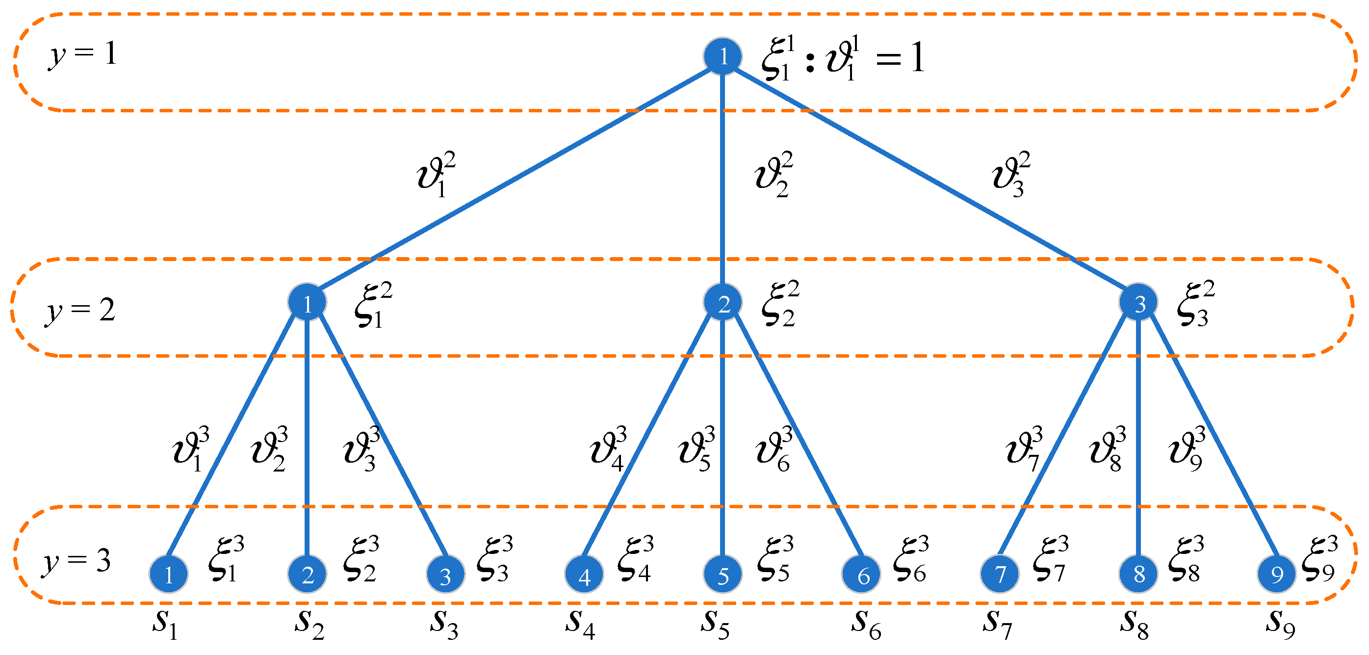
During the muti-stage planning process, the uncertainties can be observed stage by stage, and the progressive realizations of uncertainties over stages can be illustrated by the scenario tree. A typical three-stage scenario tree is taken as an example, as shown in Figure 1. The buses at each level indicate the potential realizations of the uncertainties at the corresponding planning stage, and the edges represent the transition from the upper-level scenarios to the lower-level scenarios.
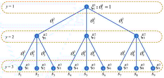
Figure 1.
The three-stage scenario tree.
In Figure 1, the number of realizations of the uncertainty at three stages is assumed as 1, 3, and 9, respectively, and these realizations are denoted as {}, {,,} and {}, respectively. Moreover, the occurrence probability of the uncertainty realization at each stage is represented as {}, {,,} and {}, respectively. Obviously, follows the equation Hence, nine planning scenarios can be generated from the three-stage scenario three, and each planning scenario consists of realizations of the uncertainty at three stages. The planning scenarios s and the corresponding probability are shown in Equation (1) and Equation (2), respectively.
It is noted that the realizations of the uncertainties at each stage can be independently generated with the mature sampling and scenario-reduction method, such as the Latin hypercube sampling method and synchronous backpropagation reduction method in [19], which is no longer introduced in detail since it is not the main contribution of this paper.
2.1.2. Decision-Making Procedure
According to the progressive realizations of the uncertainty, the planning strategy needs to be determined stage by stage to improve the planning efficiency, i.e., observing → determining the planning decision at the 1st stage → observing → determining the planning decision at the 2nd stage → … → observing → determining the planning decision at the yth stage . Hence, the planning strategy at yth stage is dependent on the realization of the uncertainty, which can be observed at yth stage , , …, , and needs to be unified for all realizations of . In other words, the same realizations of uncertainty must lead to unified planning decisions, enforced by the nonanticipativity constraints, which will be explained through a three-stage case.
A three-stage planning procedure and the corresponding nonanticipativity constraints are introduced based on the scenario tree in Figure 1. Let denote the planning decision at stage y and scenario s. At the first stage, only one realization of the uncertainty is observed, i.e., . Hence, the planning strategies for the nine planning scenarios must be unified according to the nonanticipativity constraints, as shown in Equation (3).
Then, there are three potential realizations of the uncertainty at the 2nd stage, i.e., {,,}. According to the nonanticipativity constraints, the planning decisions for the planning scenarios with the same realization of the uncertainty at the 2nd stage are unified as follows:
Hence, the nonanticipativity constraints for the y-stage s-scenario stochastic model can be derived, as shown in Equation (5):
where is the index for the realization of the uncertainty at stage y. is the set for the scenario with the same realization of the uncertainty at stage y. An example of in a three-stage, nine-scenario case, as shown in Figure 1, is presented in Equation (6):
2.2. Dynamic Frequency Stability Constraints
RGs are generally interfaced with the grid through power converters, which can participate in the frequency regulation through proper control architecture, such as the rate of change of frequency (ROCOF) loop and droop loop [20]. The transfer function of the RG frequency response is shown in Equation (7).
where is the active power increment of RG for the frequency regulation; is the increment of the system frequency; and are virtual inertia constant and droop constant of RG frequency regulation control, respectively; and indicates the time constant of the RG response.
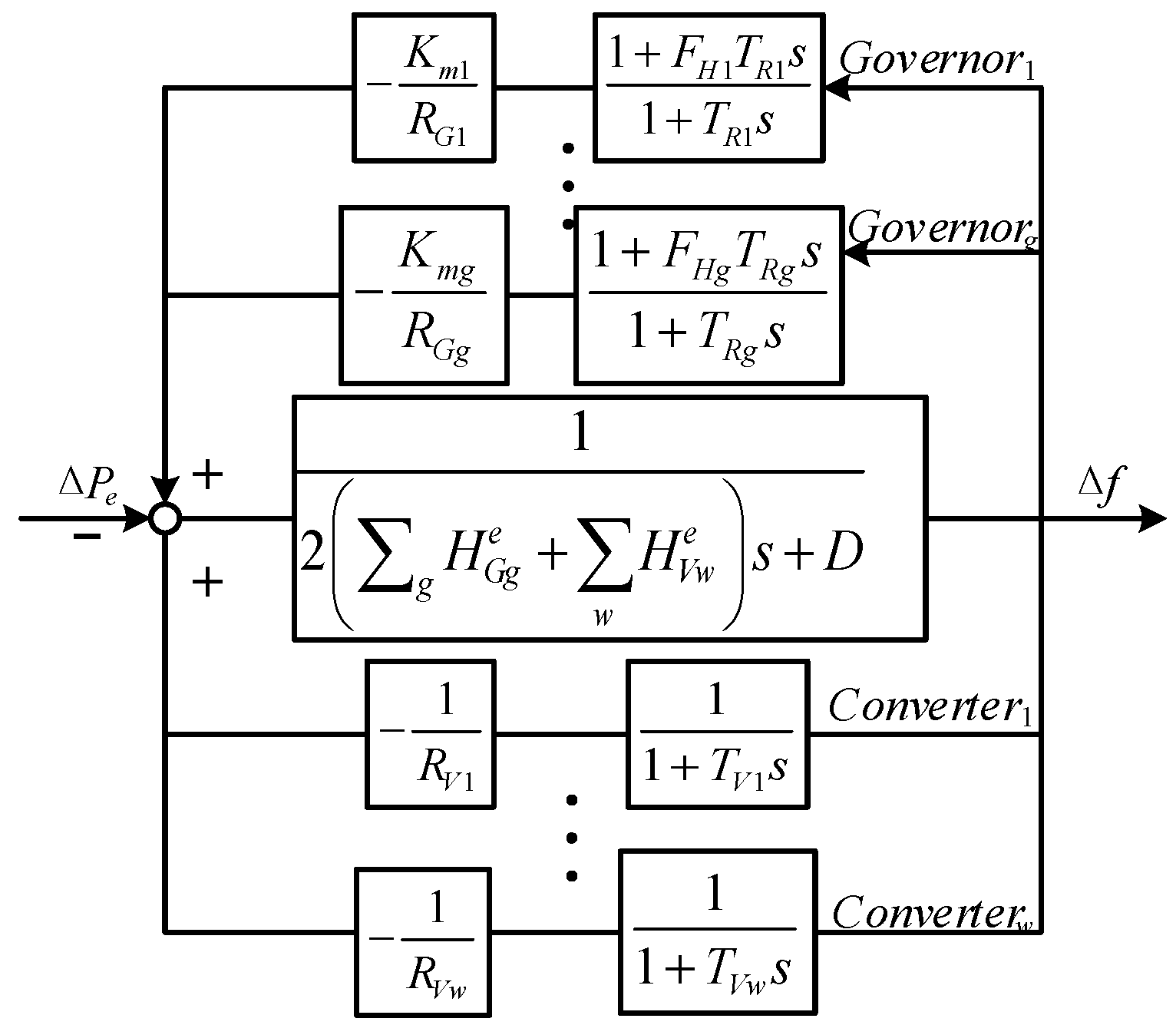
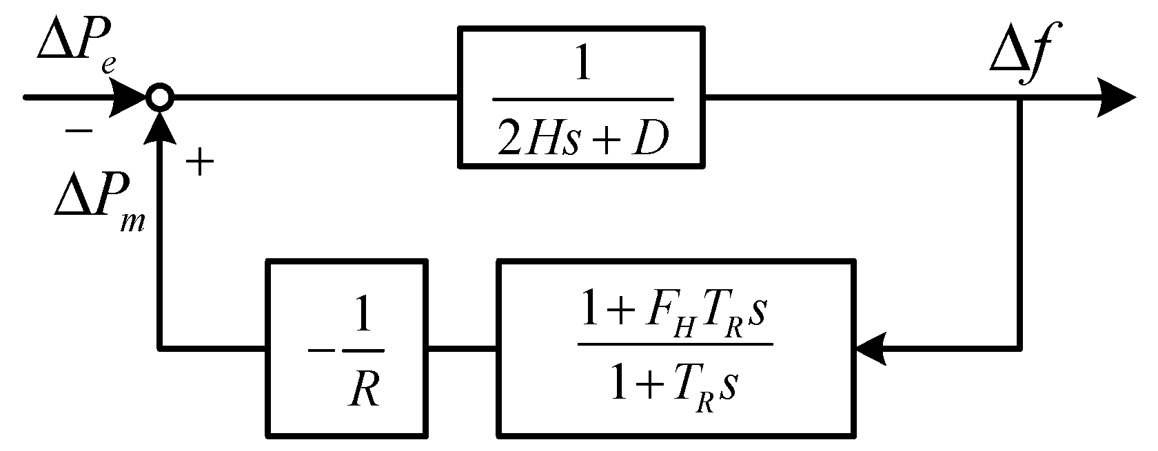
Then, a multi-machine system frequency response model considering the participation of RGs is built based on the low-order system frequency response model [2], as shown in Figure 2, where and D are the inertia constant and damping constant of the synchronous generation g, respectively; and other parameters concerning the governor response of SGs, such as , , and , can be found in [2].
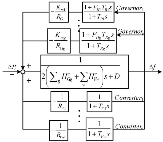
Figure 2.
Multi-machine frequency response model.
In the multi-machine system frequency response model in Figure 2, the forward path is primarily associated with the system damping D, SG inertia () and the virtual inertia provided by WTs (). The upper feedback loop represents the process in which the governor of the SGs responds to frequency deviation by increasing mechanical power output. The lower feedback loop reflects the process in which wind turbines respond to frequency deviation by increasing electrical power output.
Next, the multi-machine frequency response model can be aggregated into a single-machine model with the following steps [21]:
(1) The time constant of the RG is approximately unified to the reheating time constant of SGs (), which is a conservative assumption that guarantees the robustness of the planning strategy due to the faster response of RGs.
(2) The equivalent parameter of H, R and FH can be obtained by Equation (8), where and are the rated power of the SG g and RG w, respectively. Then, the aggregated single-machine model can be generated as follows, as shown in Figure 3:
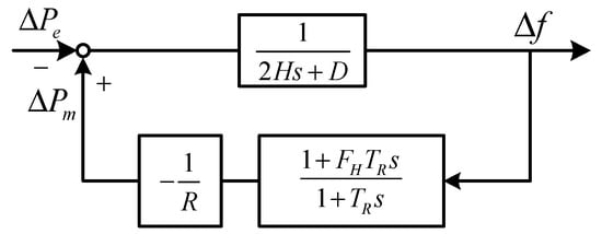
Figure 3.
The single-machine frequency response model.
Subsequently, with the step power disturbance , the dynamic frequency behaviors can be expressed in an analytical form according to Figure 3, as shown in Equation (9). The derivation and explanation for variables are provided in Appendix A.
Lastly, the constraints on dynamic frequency stability can be derived, as shown in Equation (10), including the limits on the steady frequency deviation, rate of change of frequency (RoCoF) and the frequency nadir, respectively:
where is the deviation in the steady frequency; is the deviation in the frequency nadir; and , and are the upper limits of these frequency indices, respectively.
2.3. Multi-Stage Stochastic Model Formulation
The mathematical formulation of the proposed multi-stage stochastic model for the expansion planning of TPSs is developed in this section, including the objective function (11)–(13), limits on the planning decisions over stages (14)–(16), power balance (17) and power flow (18)–(19), power outputs of RGs and SGs (20)–(22), dynamic frequency stability (10) (23)–(26) and nonanticipativity constraints (27)–(29).
2.3.1. Objective Function
The objective function of the planning model is to minimize the expectation of total capital costs, including the planning cost and the operational costs for typical days, as shown in (13):
where:
where , , , , , and are sets for buses, planning scenarios, time periods, planning stages, SGs, RGs and transmission lines, respectively. , , and are binary variables, indicating whether the line l, SG g and RG w have been built at scenario s and stage y, respectively. , , and are the capital costs for the transmission line ij, SG g and RG w, respectively. is the power outputs of SG g at scenario s, stage y and time t; is the operational costs of the SG g; is the load curtailments at bus i, scenario s, stage y and time t due to the power unbalance; and is the penalty for the power curtailments. is the occurrence probability of the scenario s; is the number of typical days; and d is the interest rate.
2.3.2. Limits on the Planning Decisions
Once an SG has been built at stage y, this SG will remain in operational condition at the following stages, as modeled in (14). This conclusion is suitable for the RG and transmission line, as shown in (15) and (16), respectively.
2.3.3. Limits on the Power Balance
The nodal power balance should be met as shown in (17), where , and are sets of SGs at bus i, RGs at bus i, and buses, respectively. is the power outputs of RG w at scenario s, stage y, and time t. is the power flow through the line ij at scenario s, stage y, and time t. is the load power at bus i, scenario s, stage y, and time t.
2.3.4. Limits on the Power Flow
The power flow constraints consist of the DC power flow model (18) and the limit on the power through the transmission line (19), where is the voltage phase of bus i at scenario s, stage y, and time t. is a large number and is the upper bound of the power through the line ij.
2.3.5. Limits on the Power Outputs of RG and SG
The power outputs of RG are limited by the forecasting value, and the power outputs of SG are constrained by the upper and lower bound of the SG power, as modeled in (20) and (21), respectively, where is the forecasting value of power output of the RG w at scenario s, stage y and time t; and and are the minimum and maximum power of SG g at scenario s, stage y, and time t, respectively. Moreover, the power output of RG is limited by the ramping capacity, as shown in (22), where is the ramping limit of SG g.
2.3.6. Dynamic Frequency Stability
The dynamic frequency stability constraints have been derived in Equation (12). Specifically in the multi-stage stochastic planning model, the equivalent parameters of H, R and FH in (12) need to be reformulated, as shown in (23)–(26).
2.3.7. Nonanticipativity Constraints
According to the nonanticipativity constraints derived in (5), the nonanticipativity constraints in the multi-stage stochastic planning model are modeled as (27)–(29).
It can be seen that the multi-stage stochastic model for the TPS expansion planning is a high-dimensional mixed-integer nonconvex model, which is significantly challenging to solve. For this purpose, the corresponding linearization and decomposition solution methods will be introduced in the following section.
3. Solution Method
An efficient solution method for the multi-stage nonconvex stochastic model is introduced in this section. First, the frequency stability constraints (12) are linearized with a maximal affine function-based piecewise linearization method in Section 3.1. Subsequently, the multi-stage multi-scenario is decomposed with the progressive hedging algorithm in Section 3.2.
3.1. Model Linearization
A maximal affine function-based piecewise linearization method is proposed in this section to address the frequency stability constraints (12). First, the maximal affine function is built, as shown in (30).
where , , , are coefficients of the ith-fitted hyperplane. m is the number of fitted hyperplanes.
Subsequently, the least-squares function is employed to capture the fitted error between the fitted hyperplanes and the original hypersurface , as shown in (31).
It can be seen that Equation (31) is actually a max–min-optimization problem, which cannot be directly solved with commercial solvers. Hence, Equation (31) is further transformed into the max-optimization problem by introducing the continuous variable and binary variable , as shown in (32).
By employing (32), the nonlinear frequency stability constraints can be represented with several hyperplanes, which can be integrated into the multi-stage planning model and improve the computational efficiency.
3.2. Model Decomposition
The dimensionality of the multi-stage stochastic model increases with the number of scenarios, which can significantly increase the computational burden. In this section, a progressive hedging algorithm is employed to decompose the multi-scenario model into several single-scenario models. First, the multi-stage stochastic model is abbreviated for the clear explanation, as shown in (33).
where and are the sets of the planning decisions and operational decisions at stage y and scenario s, respectively. is the feasible region of the system operation at stage y and scenario s., , , , are the coefficient matrices.
It can be seen from (33) that the decisions among scenarios are coupled due to the nonanticipativity constraints, i.e., the third constraint in (33). Hence, the nonanticipativity constraints are first relaxed according to the PHA method, as shown in (34).
where is the Lagrange-multiplier vectors; is the penalty for ; is the 2-norm; is the probability-weighted average of regarding scenario s, which can be calculated as (35).
It can be seen that the formulation (34) is a scenario-decoupled problem, which can be decomposed into several sub-problems with respect to scenarios. Then, these scenario-based sub-problems can be solved in parallel to improve computational efficiency. The steps of PHA to solve the multi-stage model are outlined in Algorithm 1.
| Algorithm 1: Progressive hedging algorithm | |
| , Lagrange-multiplier vectors . . | |
| (36) | |
| in (35). in (37). | |
| (37) | |
| , and repeat iteration from step 2. | |
4. Case Studies
In this section, case studies are performed in the IEEE 6-bus, 39-bus and 118-bus transmission systems. The 6-bus system is used to validate the effectiveness and superiority of the multi-stage planning model, while the 39-bus and 118-bus systems are employed to validate the effectiveness of the larger systems. All simulations are performed on the GAMS 23.7/CPLEX 12.3 computer platform with a core i5, a 3.2 GHz processor, and a 4 GB RAM.
4.1. Simulations on Six-Bus Transmission System
Numerical simulations are first conducted on the six-bus transmission system to validate the effectiveness and superiority of the proposed method. A three-stage, four-scenario stochastic planning strategy is applied for the system expansion planning, and six RGs and six SGs serve as the candidates to be built. Other parameters of the six-bus system can be found in [22].
4.1.1. Effectiveness of the Multi-Stage Planning Method
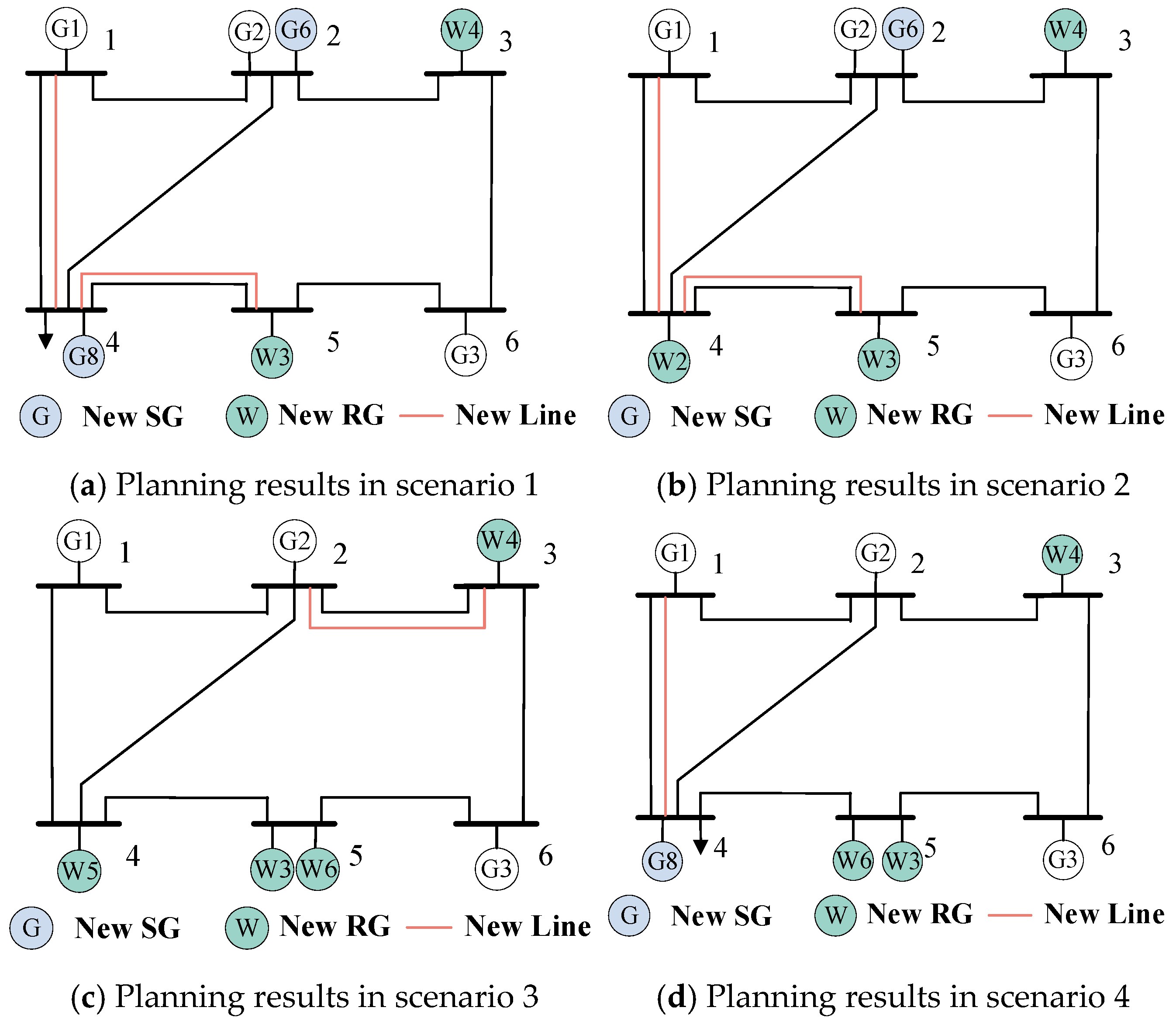
By employing the proposed multi-stage planning method, the planning results are shown in Figure 4, and the multi-stage planning decisions are presented in Table 2. According to the nonanticipativity constraints, the planning decisions among four scenarios at stage 1 should be unified, i.e., the newly-built RG W3 and W4, as shown in Table 2. Moreover, the planning decisions at stage 2 between S1 and S2 should also be identical, as shown in Table 1, i.e., the newly-built lines 1–4, 4–5, and SG G6, since the same realization of uncertainty at stage 2 is shared between S1 and S2. The same conclusion can be drawn from the decisions at stage 2 between S3 and S4. Hence, the effectiveness of the proposed method in addressing the progressive realizations of uncertainty over stages can be validated.
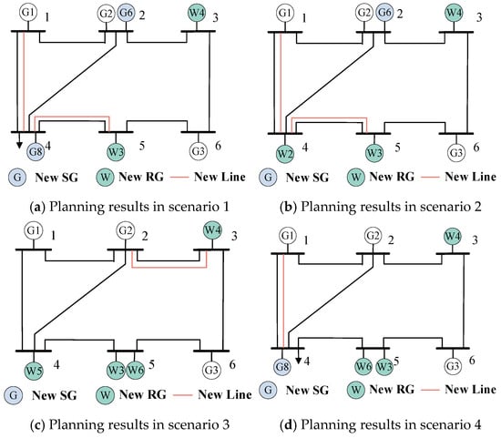
Figure 4.
Planning results in all scenarios.
Table 2.
The multi-stage planning decisions.
Then, the proposed multi-stage stochastic method is compared with the traditional two-stage model [10]. The planning results of the two-stage model are shown in Table 3, and the comparison between the multi-stage and two-stage models is shown in Table 4. It can be seen that the scenario-independent planning decisions are generated by the two-stage model, which ignores the progressive realizations of the uncertainty over stages, thereby improving the total costs by 14.6%, as shown in Table 4. Hence, the superiority of the multi-stage stochastic model can be demonstrated.
Table 3.
Two-stage planning decisions.
Table 4.
The comparison between multi-stage and two-stage models in 6-bus system.
4.1.2. Effectiveness to Address the Frequency Stability
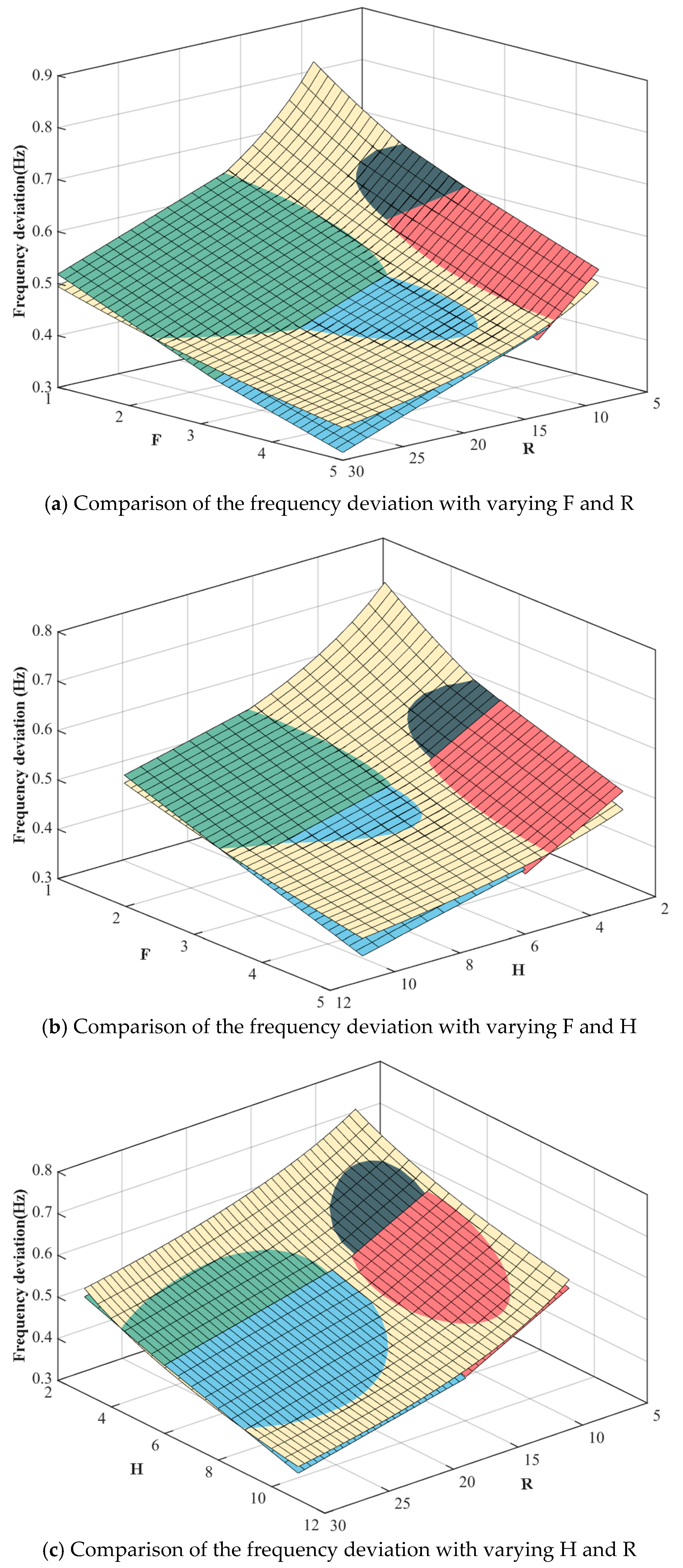
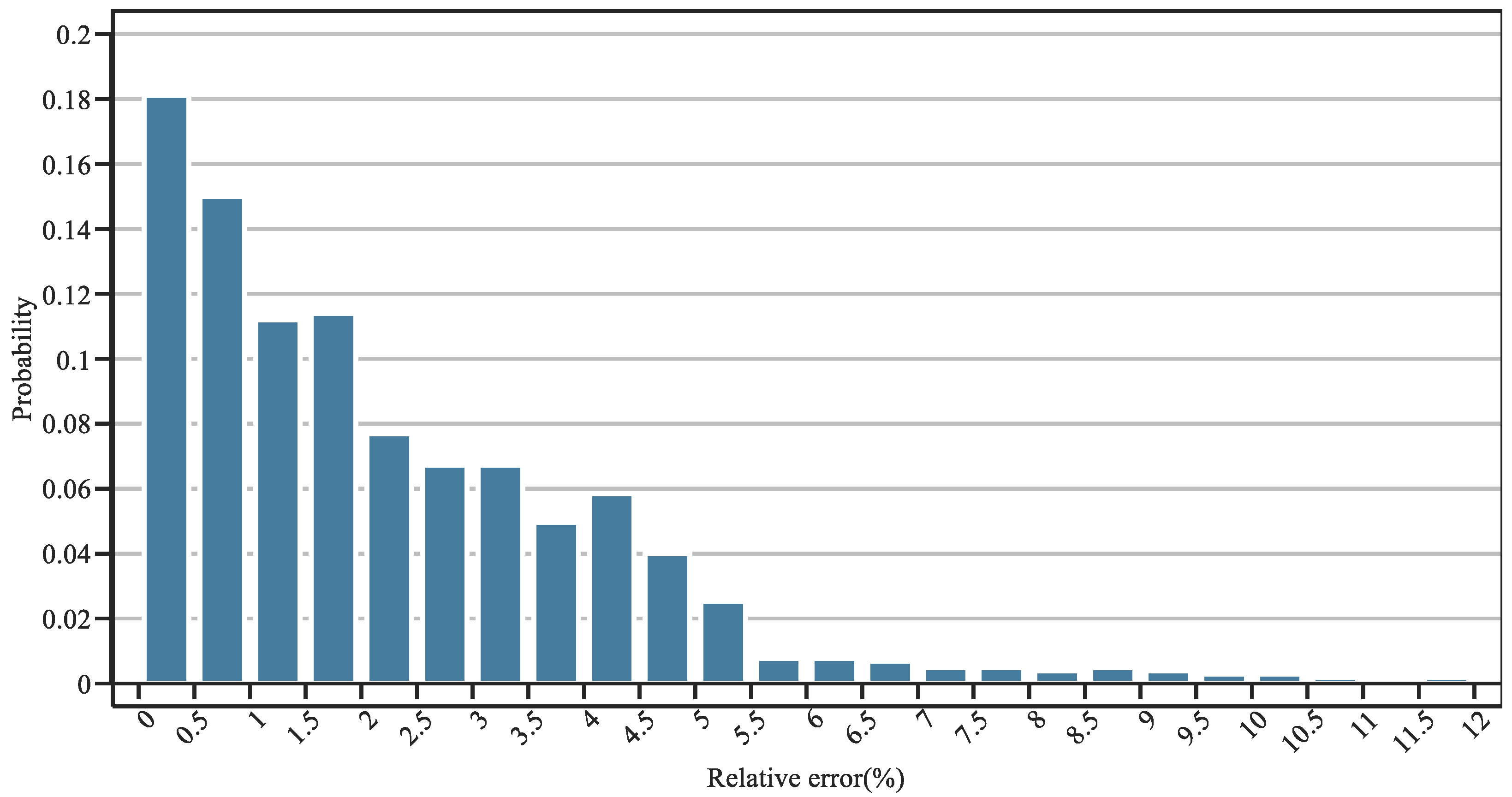
The effectiveness of the proposed method in addressing frequency stability is validated in this section. First, the effectiveness of the linearization method is discussed by illustrating the linearization errors. Specifically, the comparison of the deviation in frequency nadirs between the original and linearized function is shown in Figure 5. Moreover, 1000 data points of (H, R, F) are randomly generated to provide the probability distribution of the relative error, as shown in Figure 6. It can be seen that the relative error can be limited in the range of [0, 5.5%] with a confidence of 96.4%, and the expectation of the relative error is 1.37%, showing the effectiveness of the linearization method.
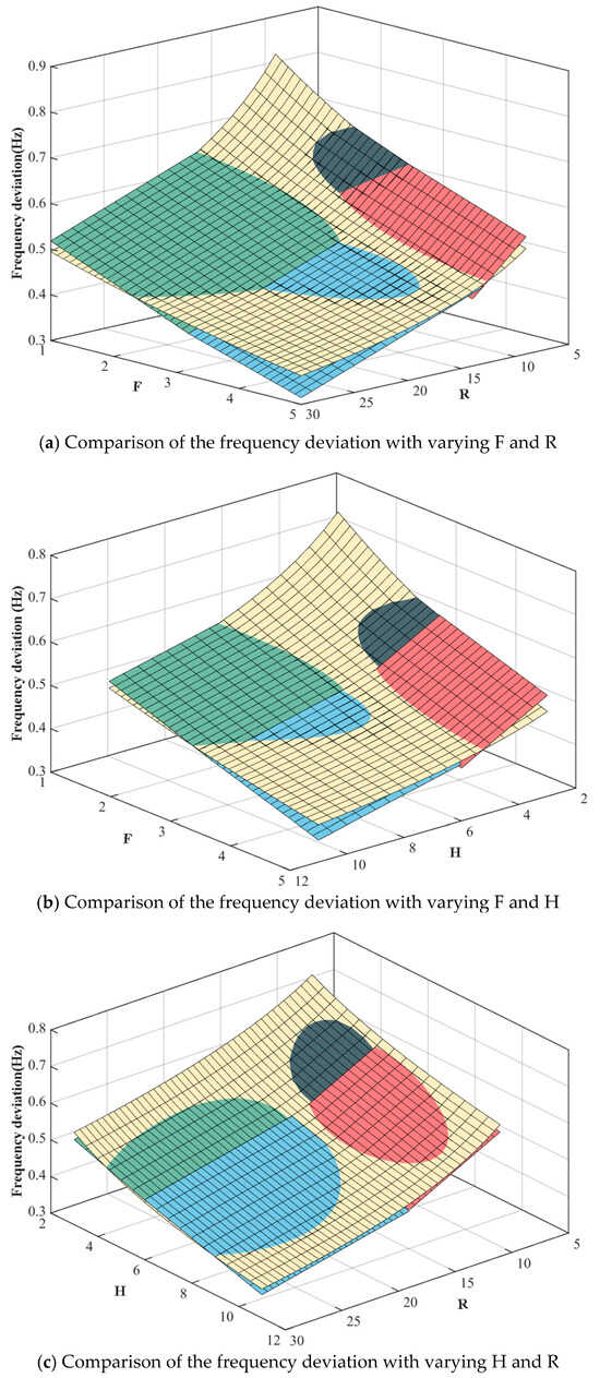
Figure 5.
Comparison of the frequency deviation with varying F, R and H.

Figure 6.
Probability distribution of the relative error.
Subsequently, the linearized frequency stability constraints are integrated into the three-stage planning model (denoted as FC-PL), and the planning decision is compared with that of the model with no consideration of dynamic frequency constraints (denoted as NFC-PL) [23]. To ensure the fairness of the comparison test, the controlled experiment is adopted, as shown in Table 5. Specifically, the candidates, uncertainty model, objective function, operational constraints and solution algorithm are set to be identical except for the dynamic frequency constraints.
Table 5.
The controlled experiment for the comparison of FC-PL and NFC-PL.
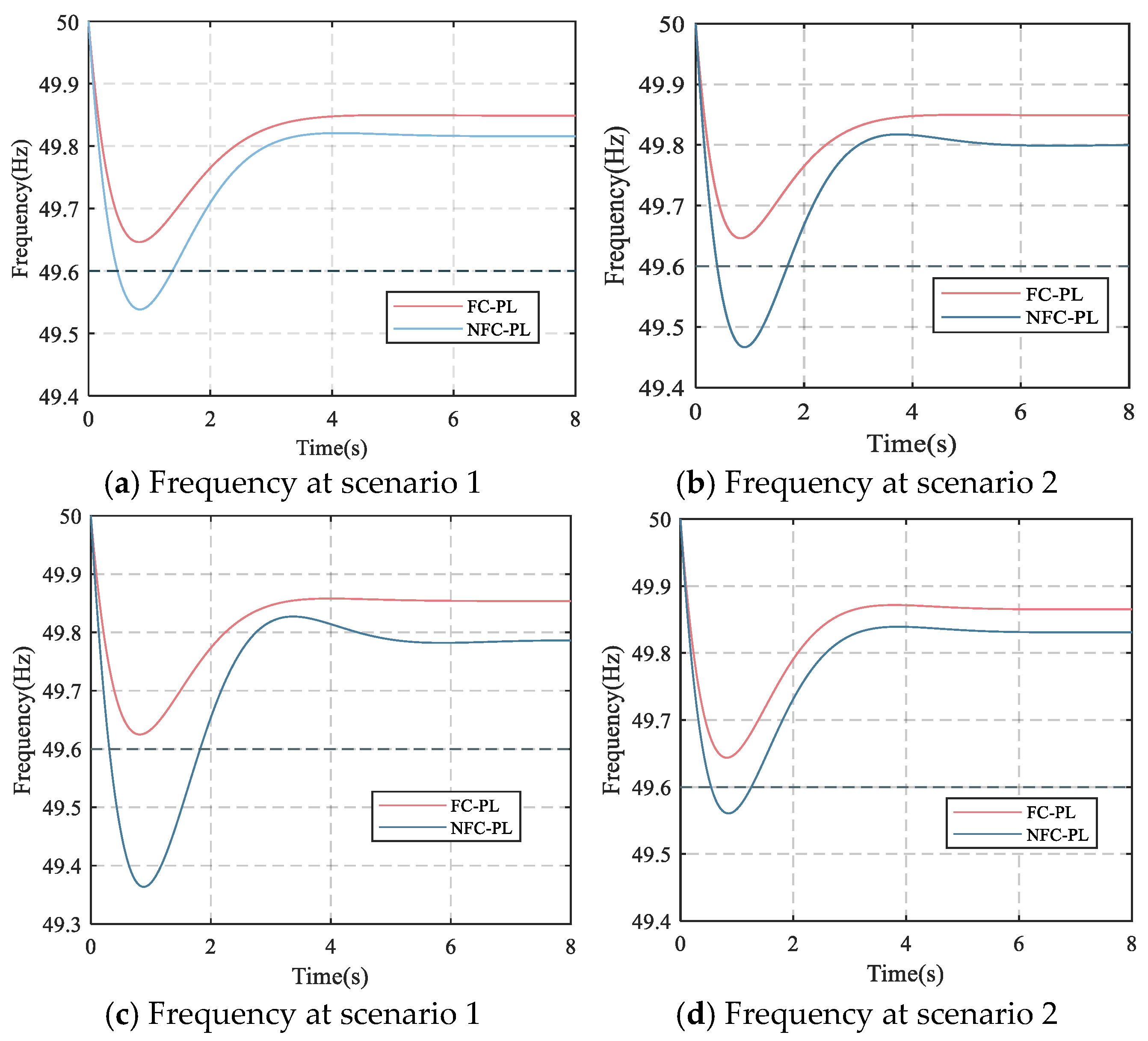
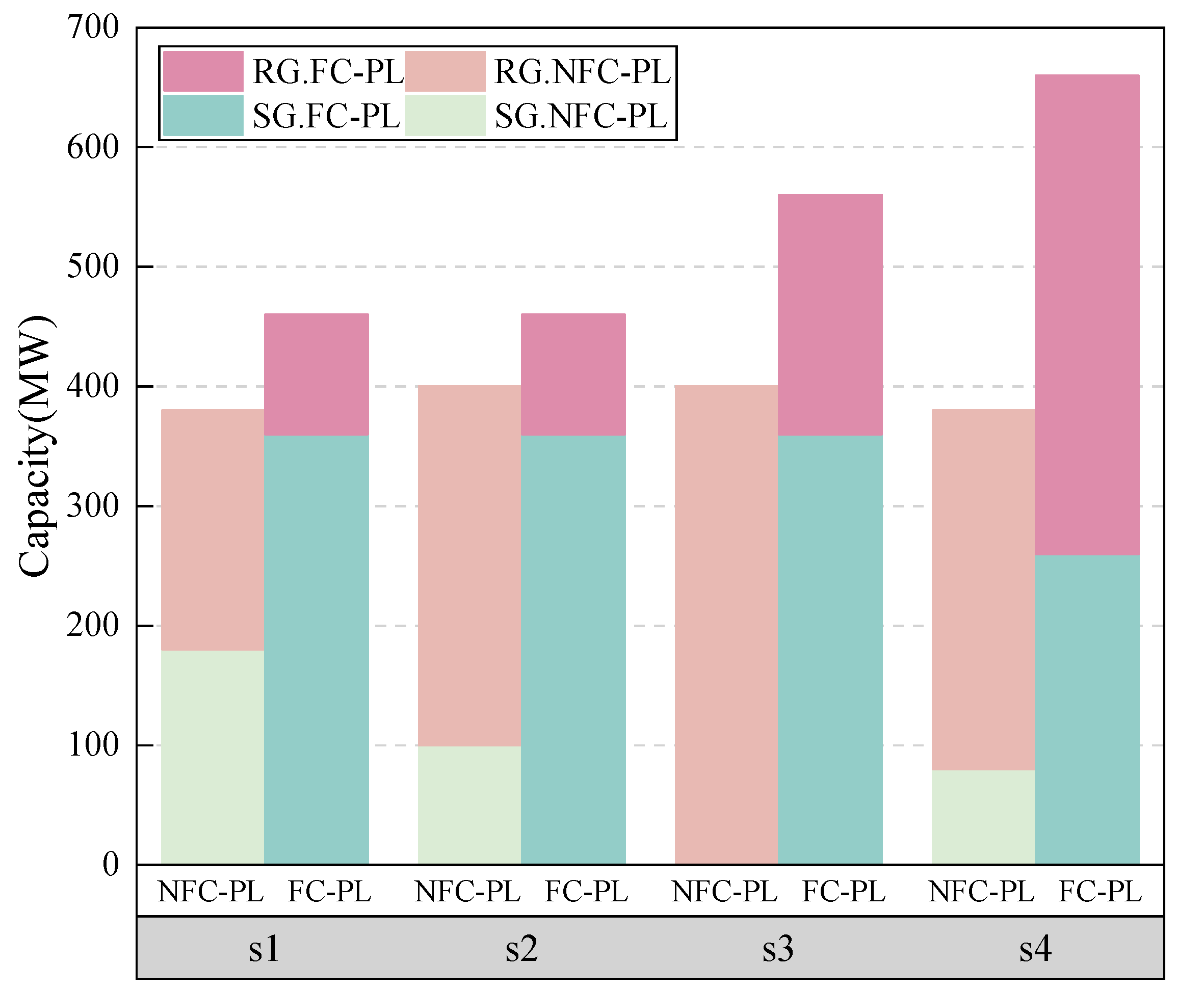
The effectiveness of addressing the frequency stability is compared by the frequency curves in Figure 7 and frequency stability indices in Table 6. The limits on the fnadir, RoCoF and fss are 49.6 Hz, 0.5 Hz/s and 49.85 Hz, respectively. It can be seen that the frequency stability indices, including fnadir, RoCoF and fss, deviate from the limited range in the NFC-PL. In contrast, the dynamic frequency stability can be strictly guaranteed by employing the proposed method since the RGs are deployed in coordination with the SGs with a strong capacity for frequency regulation rather than the blind deployment of RGs in the NFC-PL method, as shown in Figure 8.
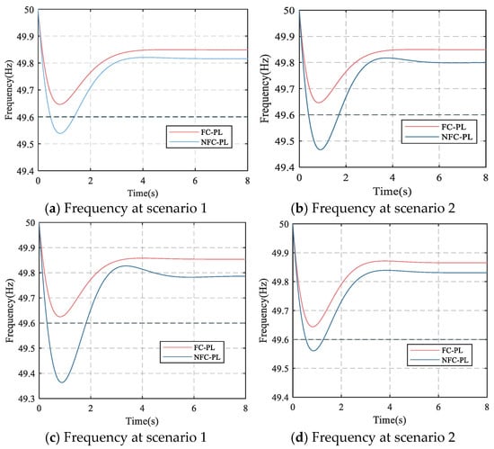
Figure 7.
Frequency at all scenarios.
Table 6.
The critical indices of frequency stability.
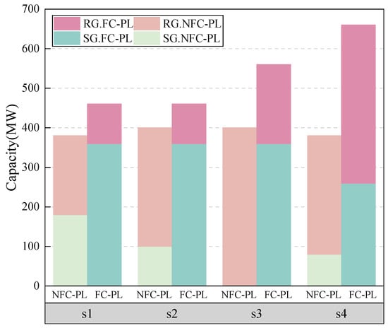
Figure 8.
Comparison between models with/without frequency stability.
Moreover, the frequency dynamics can be explained as follows. The frequency response process of power systems primarily consists of three stages: inertial response, primary frequency control, and secondary frequency control. When a disturbance occurs, the system’s frequency rapidly declines. First, the inertial response is provided by synchronous generators, which react to the RoCoF by quickly releasing stored rotational kinetic energy, thereby alleviating the rate of frequency decline. Subsequently, primary frequency control is activated by governors of SGs to improve the active power output in response to frequency deviations. However, primary control alone cannot restore frequency to its nominal value due to its limited regulation capability. Finally, secondary frequency control, implemented via the Automatic Generation Control (AGC) system, coordinates the outputs of multiple generating units based on Area Control Error (ACE), which considers both frequency deviation and tie-line power deviation. This process occurs over a period of several tens of seconds to a few minutes, effectively restoring the frequency to its nominal value and maintaining power balance. This paper focuses on the frequency security issues during the inertial response and primary control stages; thus, the system frequency in Figure 7 does not recover to the nominal value.
4.1.3. Effectiveness of the Decomposition Method
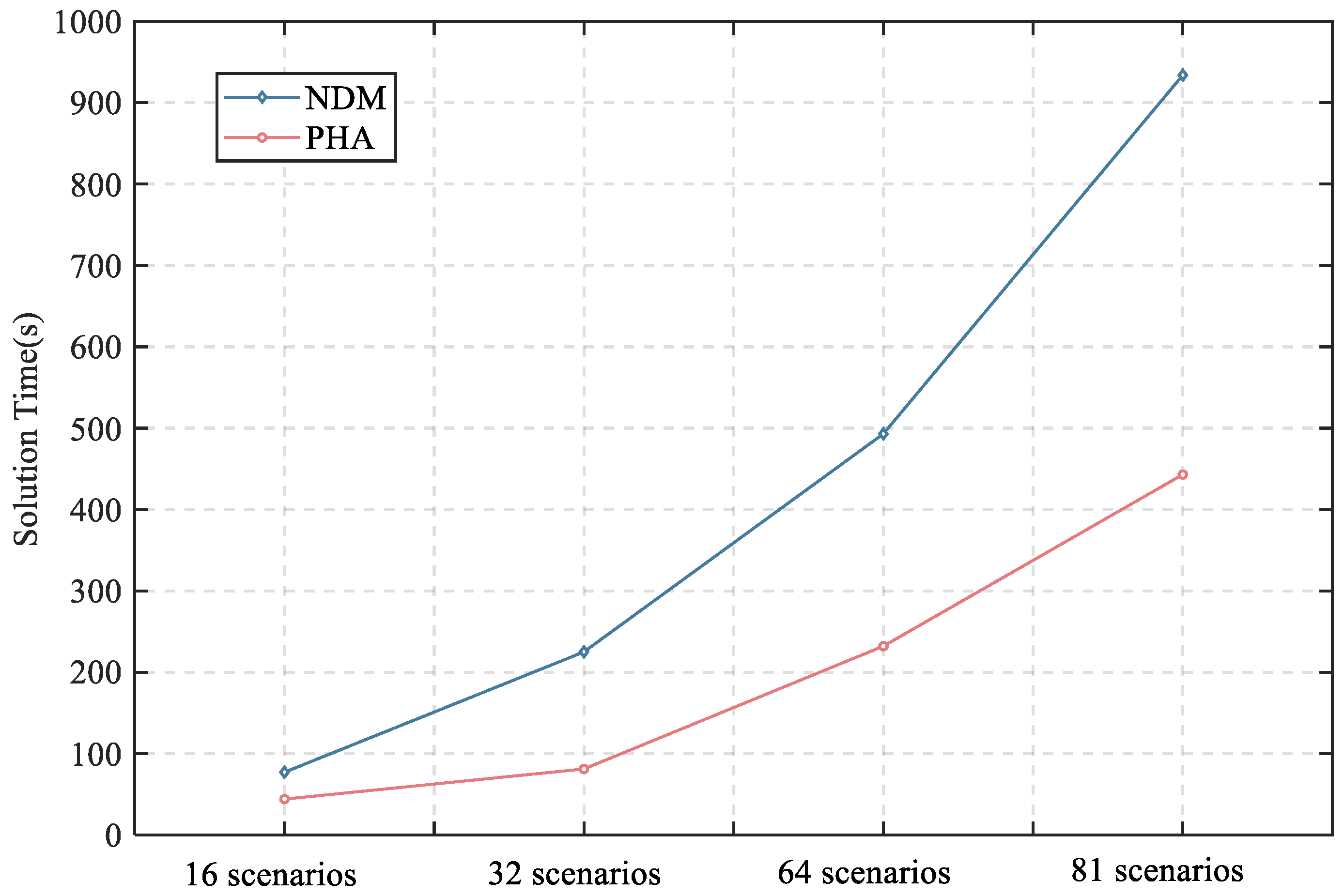
The effectiveness of the PHA decomposition method is demonstrated in this section. First, the optimality of the PHA method is discussed by comparison with the non-decomposition method (NDM), and the comparison results are shown in Table 7. It can be observed that, compared to the NDM algorithm, which is a centralized solution method, the proposed algorithm does not achieve the global optimal solution. This is because the PHA algorithm is a heuristic approach and thus typically yields only near-optimal solutions. However, the solution obtained by the PHA algorithm has a deviation of only 0.94%, which is acceptable for planning purposes. The main advantage of the PHA algorithm lies in its ability to reduce computational burden through model decomposition, as shown in Figure 9. It can be seen that the computational burden can be reduced by at least 43% while generating a high-quality solution with a small relative error of 0.94%, and the improvement for the computational efficiency is highlighted for the high-dimensional model with massive scenarios, as illustrated in Figure 9.
Table 7.
The comparison between PHA and NDM method in 6-bus system.
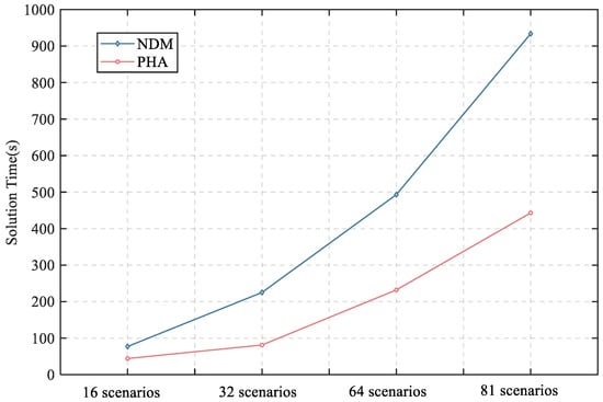
Figure 9.
Comparison of solution time with different amounts of scenarios.
4.2. Simulations on 39-Bus and 118-Bus Transmission Systems
The numerical tests are further conducted on the larger 39-bus and 118-bus transmission systems to validate the effectiveness of the proposed method. First, the proposed multi-stage model is compared with the two-stage model, as shown in Table 8. It can be seen that the total costs can be reduced by 16.3% and 21.4% for the 39- and 118-bus systems, respectively, showing the superiority of the multi-stage model for the progressive uncertainty. Moreover, the frequency stability indices of the 39- and 118-bus systems are shown in Table 9 and Table 10, respectively, and the comparison between the FC-PL and NFC-PL models, including the WTs, photovoltaic generation (PV) and SGs, is illustrated in Figure 10, which shows the effectiveness of the proposed FC-PL model to guarantee the dynamic frequency stability by properly determining the proportion of RGs and SGs.
Table 8.
The comparison between multi-stage and two-stage models in 39- and 118-bus systems.
Table 9.
Critical indices of frequency stability in the 39-bus system.
Table 10.
Critical indices of frequency stability in the 118-bus system.
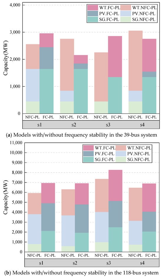
Figure 10.
Models with/without frequency stability in the 39-bus and 118-bus systems.
Lastly, the effectiveness of the proposed PHA decomposition method is demonstrated. The convergence behaviors of the PHA method in the 39-bus and 118-bus systems are provided in Figure 11, and the comparison between the PHA and NDM methods concerning the optimality and solution efficiency is shown in Table 11. It can be seen that the PHA decomposition method can converge in 19 and 77 iterations in the 39-bus and 118-bus systems, respectively. Moreover, the high-quality solution can be obtained with relative errors of 3.2% and 4.5% by employing the PHA method while improving the computational efficiency significantly by 77.8% and 84.5% in the 39- and 118-bus systems, respectively.
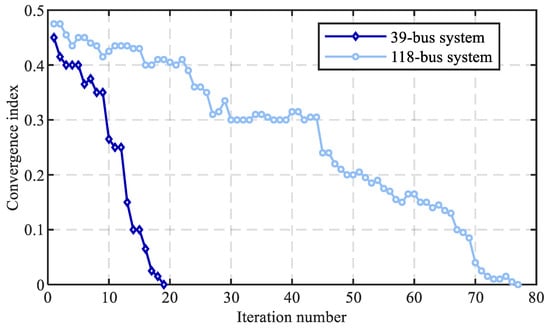
Figure 11.
Convergence behaviors of the PHA method in the 39-bus and 118-bus systems.
Table 11.
The comparison between PHA and NDM methods in 39- and 118-bus systems.
5. Discussion
This paper proposes a multi-stage stochastic planning method for TPSs considering dynamic frequency stability, which can improve the symmetry of RGs and SGs in modern power systems. In this scheme, the progressive uncertainties over stages are addressed with a multi-stage stochastic method with nonanticipativity constraints, which can reduce the capital and operational costs by 21%. Moreover, the dynamic frequency stability constraints are derived and integrated into the planning model, which can guarantee frequency stability by properly arranging the proportion of RGs and SGs according to the numerical simulations. Furthermore, a PHA decomposition method is designed to reduce the computational burden of the proposed model, which can improve computational efficiency significantly by 84.5% with relative errors of 0.94%. Therefore, optimality, solvability, and implementation can be significantly improved by employing the proposed planning approach.
The frequency regulation model of WTs developed in this study is based on the assumption that sufficient frequency reserves are retained. However, wind turbines typically operate in Maximum Power Point Tracking (MPPT) mode to capture as much wind power as possible, which can lead to a secondary frequency drop after participating in frequency regulation. Future research should, therefore, focus on power system planning and operation models that take secondary frequency drops into account. In addition, overcurrent due to excessive short-circuit current is another critical challenge in the planning of renewable-dominated power systems, which will also be addressed in future studies.
Author Contributions
Methodology, X.L., H.S., G.Z., G.Q., W.L. and T.Z.; Software, H.S., Z.L. and Y.X.; Validation, G.Q., Y.X., Z.L. and T.Z.; Formal analysis, X.L., H.S., G.Z., Y.X. and W.L.; Investigation, X.L., G.Z., G.Q., Y.X., Z.L., W.L. and T.Z.; Resources, X.L., G.Z., G.Q., Y.X. and T.Z.; Data curation, G.Z., G.Q., Y.X., W.L., Z.L. and T.Z.; Writing—original draft, X.L., G.Q. and W.L.; Supervision, G.Z., Z.L. and G.Q.; Project administration, G.Z. and Z.L.; Funding acquisition, X.L., H.S. and G.Z. All authors have read and agreed to the published version of the manuscript.
Funding
This research was funded by the Science and Technology Project of State Grid Corporation of China (5100-202355385A-2-3-XG).
Data Availability Statement
The original contributions presented in this study are included in the article. Further inquiries can be directed to the corresponding author.
Conflicts of Interest
Author Xiaoming Luan, Huadong Sun, Guoliang Zhao, Guangyao Qiao, Zhengang Lu, Yunfei Xu and Weiguo Li were employed by the company State Grid Corporation of China. The remaining authors declare that the research was conducted in the absence of any commercial or financial relationships that could be construed as a potential conflict of interest. The authors declare that this study received funding from the Science and Technology Project of State GridCorporation of China (5100-202355385A-2-3-XG). The funder was not involved in the study design, collection, analysis, interpretation of data, the writing of this article or the decision to submit it for publication.
Appendix A
According to the single-machine frequency response model in Figure 3, the frequency response with the step power disturbance can be computed as Equation (A1).
Subsequently, Equation (A1) is reformulated into the standard formulation, as shown in Equation (A2).
Equation (A3) can then be obtained from Equation (A2) through the Inverse Laplace transform; Equation (9) can, hence, be derived.
where:
where:
References
- Zhang, G.; Zhang, F.; Meng, K.; Dong, Z.Y. A distributed calculation method for robust day-ahead scheduling of integrated electricity-gas systems. Int. J. Electr. Power Energy Syst. 2022, 136, 107636. [Google Scholar] [CrossRef]
- Zhang, G.; Zhang, F.; Ding, L.; Meng, K.; Dong, Z.Y. Wind Farm Level Coordination for Optimal Inertial Control with a Second-Order Cone Predictive Model. IEEE Trans. Sustain. Energy 2021, 12, 2353–2366. [Google Scholar] [CrossRef]
- Golshani, A.; Sun, W.; Zhou, Q.; Zheng, Q.P.; Hou, Y. Incorporating Wind Energy in Power System Restoration Planning. IEEE Trans. Smart Grid 2019, 10, 16–28. [Google Scholar] [CrossRef]
- Hu, J.; Xu, X.; Ma, H.; Yan, Z. Distributionally Robust Co-optimization of Transmission Network Expansion Planning and Penetration Level of Renewable Generation. J. Mod. Power Syst. Clean Energy 2022, 10, 577–587. [Google Scholar] [CrossRef]
- Roldán, C.; Mínguez, R.; García-Bertrand, R.; Arroyo, J.M. Robust Transmission Network Expansion Planning Under Correlated Uncertainty. IEEE Trans. Power Syst. 2019, 34, 2071–2082. [Google Scholar] [CrossRef]
- Yin, S.; Wang, J. Generation and Transmission Expansion Planning Towards a 100% Renewable Future. IEEE Trans. Power Syst. 2022, 37, 3274–3285. [Google Scholar] [CrossRef]
- Liu, Y.; Liu, T. Research on System Planning of Gas-Power Integrated System Based on Improved Two-Stage Robust Optimization and Non-Cooperative Game Method. IEEE Access 2021, 9, 79169–79181. [Google Scholar] [CrossRef]
- Alshamrani, A.M.; El-Meligy, M.A.; Sharaf, M.A.F.; Saif, W.A.M.; Awwad, E.M. Transmission Expansion Planning Considering a High Share of Wind Power to Maximize Available Transfer Capability. IEEE Access 2023, 11, 23136–23145. [Google Scholar] [CrossRef]
- Zhuo, Z.; Du, E.; Zhang, N.; Kang, C.; Xia, Q.; Wang, Z. Incorporating Massive Scenarios in Transmission Expansion Planning with High Renewable Energy Penetration. IEEE Trans. Power Syst. 2020, 35, 1061–1074. [Google Scholar] [CrossRef]
- Alnowibet, K.A.; Alrasheedi, A.F.; Alshamrani, A.M. Integrated stochastic transmission network and wind farm investment considering maximum allowable capacity. Electr. Power Syst. Res. 2023, 215, 108961. [Google Scholar] [CrossRef]
- Nguyen, N.; Almasabi, S.; Bera, A.; Mitra, J. Optimal Power Flow Incorporating Frequency Security Constraint. IEEE Trans. Ind. Appl. 2019, 55, 6508–6516. [Google Scholar] [CrossRef]
- Chu, Z.; Markovic, U.; Hug, G.; Teng, F. Towards Optimal System Scheduling with Synthetic Inertia Provision from Wind Turbines. IEEE Trans. Power Syst. 2020, 35, 4056–4066. [Google Scholar] [CrossRef]
- Wang, L.; Fan, H.; Liang, J.; Xu, L.; Li, T.; Luo, P.; Hu, B.; Xie, K. Multi-Area Frequency-Constrained Unit Commitment for Power Systems with High Penetration of Renewable Energy Sources and Induction Machine Load. J. Mod. Power Syst. Clean Energy 2024, 12, 754–766. [Google Scholar] [CrossRef]
- Carrión, M.; Dvorkin, Y.; Pandžić, H. Primary Frequency Response in Capacity Expansion with Energy Storage. IEEE Trans. Power Syst. 2018, 33, 1824–1835. [Google Scholar] [CrossRef]
- Cai, X.; Zhang, N.; Du, E.; An, Z.; Wei, N.; Kang, C. Low Inertia Power System Planning Considering Frequency Quality Under High Penetration of Renewable Energy. IEEE Trans. Power Syst. 2024, 39, 4537–4548. [Google Scholar] [CrossRef]
- Li, H.; Qiao, Y.; Lu, Z.; Zhang, B.; Teng, F. Frequency-Constrained Stochastic Planning Towards a High Renewable Target Considering Frequency Response Support from Wind Power. IEEE Trans. Power Syst. 2021, 36, 4632–4644. [Google Scholar] [CrossRef]
- Zhang, C.; Liu, L.; Cheng, H.; Liu, D.; Zhang, J.; Li, G. Frequency-constrained Co-planning of Generation and Energy Storage with High-penetration Renewable Energy. J. Mod. Power Syst. Clean Energy 2021, 9, 760–775. [Google Scholar] [CrossRef]
- Zhang, G.; Zhang, F.; Zhang, X.; Wang, Z.; Meng, K.; Dong, Z.Y. Mobile Emergency Generator Planning in Resilient Distribution Systems: A Three-Stage Stochastic Model with Nonanticipativity Constraints. IEEE Trans. Smart Grid 2020, 11, 4847–4859. [Google Scholar] [CrossRef]
- Luo, F.; Bu, Q.; Ye, Z.; Yuan, Y.; Gao, L.; Lv, P. Dynamic Reconstruction Strategy of Distribution Network Based on Uncertainty Modeling and Impact Analysis of Wind and Photovoltaic Power. IEEE Access 2024, 12, 64069–64078. [Google Scholar] [CrossRef]
- Zhang, J.; Zhang, B.; Li, Q.; Zhou, G.; Wang, L.; Li, B.; Li, K. Fast Frequency Regulation Method for Power System with Two-Stage Photovoltaic Plants. IEEE Trans. Sustain. Energy 2022, 13, 1779–1789. [Google Scholar] [CrossRef]
- Shi, Q.; Li, F.; Cui, H. Analytical Method to Aggregate Multi-Machine SFR Model with Applications in Power System Dynamic Studies. IEEE Trans. Power Syst. 2018, 33, 6355–6367. [Google Scholar] [CrossRef]
- Yuan, Y.; Zhang, Y.; Wang, J.; Liu, Z.; Chen, Z. Enhanced Frequency-Constrained Unit Commitment Considering Variable-Droop Frequency Control From Converter-Based Generator. IEEE Trans. Power Syst. 2023, 38, 1094–1110. [Google Scholar] [CrossRef]
- Orfanos, G.A.; Georgilakis, P.S.; Hatziargyriou, N.D. Transmission Expansion Planning of Systems with Increasing Wind Power Integration. IEEE Trans. Power Syst. 2013, 28, 1355–1362. [Google Scholar] [CrossRef]


Disclaimer/Publisher’s Note: The statements, opinions and data contained in all publications are solely those of the individual author(s) and contributor(s) and not of MDPI and/or the editor(s). MDPI and/or the editor(s) disclaim responsibility for any injury to people or property resulting from any ideas, methods, instructions or products referred to in the content. |
© 2025 by the authors. Licensee MDPI, Basel, Switzerland. This article is an open access article distributed under the terms and conditions of the Creative Commons Attribution (CC BY) license (https://creativecommons.org/licenses/by/4.0/).