Article

Improvement of Microwave Heating Uniformity Using Symmetrical Stirring

1
College of Electronics and Information Engineering, Taiyuan University of Science and Technology, Taiyuan 030024, China
2
College of General Education, Beijing Vocational College of Agriculture, Beijing 102208, China
*
Author to whom correspondence should be addressed.
Symmetry 2025, 17(5), 659; https://doi.org/10.3390/sym17050659
Submission received: 10 February 2025 / Revised: 18 April 2025 / Accepted: 23 April 2025 / Published: 26 April 2025
(This article belongs to the Section Engineering and Materials)

Abstract

:
This study proposes a new method of symmetrical stirring using an anchor paddle to improve the heating uniformity of liquids. To simulate the complex physical process of microwave heating a fluid while stirring it, the finite element method (FEM) and the arbitrary Lagrangian–Eulerian (ALE) method were utilised to model the interactions between electromagnetics, heat transfer, and fluid flow. The temperature coefficient of variation (COV) of the water when subjected to microwave heating and the symmetrical stirring paddle decreased by an 11.2–81.5% compared to that achieved by the traditional rotating turntable method, and it further decreased as the stirring frequency increased. This implies that the stirring method performed more favourably than the rotation method in improving the uniformity of the microwave heating. The distributions of the three physical fields indicated that symmetrical stirring enhanced the axial fluid flow and heat transfer, reducing the large intrinsic temperature difference along the vertical direction. Furthermore, the computation results were validated experimentally, showing that the proposed method is sufficiently accurate for evaluating the uniformity of microwave heating.

1. Introduction

Volumetric heating using microwave, ultrasonic, or infrared radiation has demonstrated promising potential in industrial applications owing to its rapid heating, energy conservation, and environmental friendliness [1,2]. As one of the most commonly used volumetric heating methods, microwave heating also offers other advantages, including highly efficient heating, penetrative heating, and ease of control [3,4,5,6,7,8]. Owing to these advantages, microwave heating has drawn significant attention in recent years and has demonstrated significant potential in food engineering [9,10,11], environmental engineering [12,13,14], chemical engineering [15,16,17] and medical engineering [18]. However, non-uniform heating, which is one of its major drawbacks, often produces negative results. For example, in food engineering, non-uniform heating may result in taste deterioration, nutritional loss, and microbial residues, even generating harmful substances [19]. In environmental engineering, it can lead to incomplete handling and inhibition of microbial activity [20]. In chemical engineering, it may generate incomplete reactions or additional side reactions, thereby lowering the yield and purity of the target products [21]. In medical engineering, it can result in incomplete tumour treatment and cause thermal injury to normal tissue [22]. Therefore, the negative impact of non-uniform heating severely hinders the widespread application of microwave radiation as an ideal green and pollution-free energy source in industries [23].
To overcome the problem of non-uniform microwave heating, a lot of theoretical and experimental research has been conducted [24,25,26]. The most common method employs a rotating turntable, which is beneficial for obtaining uniform temperature profiles for microwave heating applications. Zhu et al. adopted the arbitrary Lagrangian–Eulerian (ALE) method to investigate the temperature distribution and microwave pyrolysis characteristics of oil shale undergoing rotational motion. They found the temperature distribution inside the oil shale was effectively homogenised by rotational motion, and thereby the oil yield was increased to 50.12% [27]. In addition, Wang et al. improved the uniformity of radio frequency heating via tilting and rotation. The simulation and experimental results showed that when the rotational speed varied from 0 to 8 rad/min, the maximum temperature difference was reduced from 37 °C to 18.7 °C [28]. Furthermore, Yang et al. evaluated the function of a turntable under various conditions with modelling tools. The results demonstrated that rotating food impacted the heating results, primarily by reducing the temperature difference between the hot and cold regions [29]. Moreover, Shen et al. investigated the microwave transmission mode and route for a sample of germinated brown rice (GBR), accounting for its rotation and the presence of pores within it, and further analysed the heating uniformity. They demonstrated that rotation improved the uniformity of the temperature distribution of the bulk GBR in the equatorial direction (rather than in the radial direction) as it was microwave-dried on the turntable [30]. However, rotation barely enhanced the uniformity of heating across the different layers of the substance. The electromagnetic field varies since the dielectric properties of the sample are temperature dependent [31,32,33]. Therefore, developing other technologies to obtain more uniform temperature profiles in both the horizontal and vertical directions is required.
This study proposes a new method of stirring using an anchor paddle, which improves the heating uniformity by producing forced convection along both the horizontal and vertical directions inside the liquid as it is microwave heated. To simulate the complex physical process of microwave heating a fluid while stirring it, the finite element method (FEM) and the arbitrary Lagrangian–Eulerian (ALE) method, which has the ability to adjust to variations in the solution domain caused by mesh rebuilding or morphing due to the stirring of the paddle, was utilised to model the interactions between the electromagnetics, heat transfer, and fluid flow. Capitalizing on the proposed method, a three-dimensional multi-physics calculation model was used to investigate the temperature uniformity and velocity profiles of water heated with a stirring paddle revolving at different stirring frequencies, and the results were compared to those for a rotating turntable. Finally, experiments were conducted to validate the applicability of the proposed mathematical model.

2. Methodology

2.1. Multi-Physics Simulation
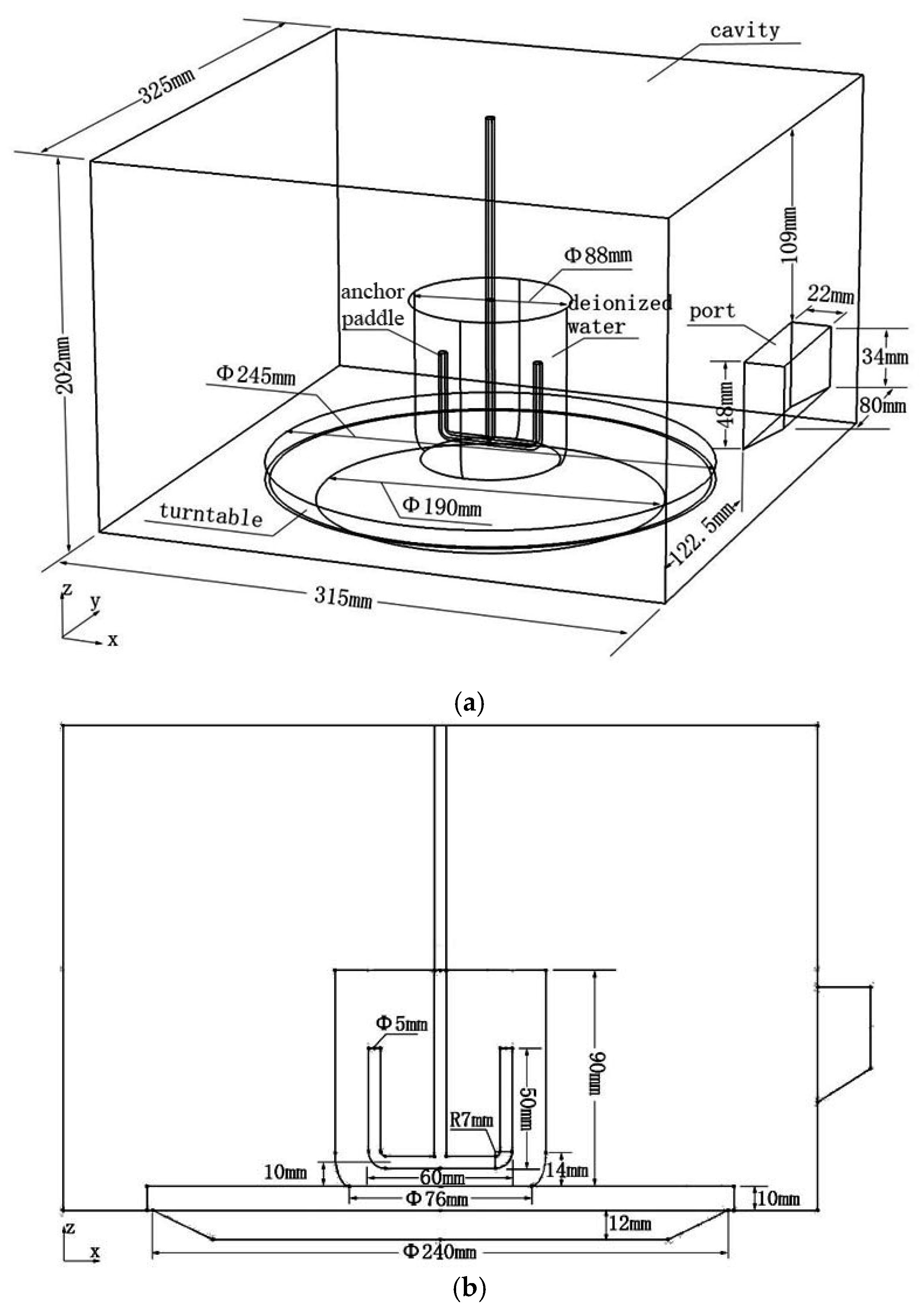
2.1.1. Geometry

The three-dimensional (3D) geometry consistent with the experimental system is given in Figure 1. A Midea household microwave oven (M1-211A, Midea Microwave Oven Manufacturing Co., Ltd., Foshan, China) with a TE10 mode was used for this study, and its internal dimensions were 315 mm × 325 mm × 202 mm. It was operated at a frequency of 2.45 GHz with a maximum output power of 700 W. The microwaves were transmitted along a rectangular waveguide with external dimensions of 80 mm × 22 mm. A glass turntable with a thickness of 10 mm was placed at the bottom of the oven. A 500 mL glass beaker with an internal diameter of 88 mm was situated centrally on the turntable and filled with deionised water (Nongfu Spring Co., Ltd., Hangzhou, China). The curves of the bottom of the beaker were approximately a quarter of an elliptical curve with a semi-major axis of 14 mm and a semi-minor axis of 6 mm. To simplify the model, the thickness of the beaker was neglected. A glass anchor paddle with dimensions of 60 mm × 50 mm × 5 mm was placed at the centre of the beaker along the vertical plane at a height of 10 mm from the bottom of the beaker. The paddle was stirred clockwise along the z-axis. The same geometric model but without the stirring paddle was applied to emulate the heating process with a rotating turntable.
The integrated Maxwell equations, heat conduction equation, and fluid dynamics equations were addressed collectively to model the microwave heating. The ALE method was employed to handle the deformation of the boundary caused by the stirring of the anchor paddle. A frequency-transient solver was one of the preset solvers in the software; hence, it was used to solve the coupled equations of the multi-physics and auto re-meshing of the time-dependent boundary.

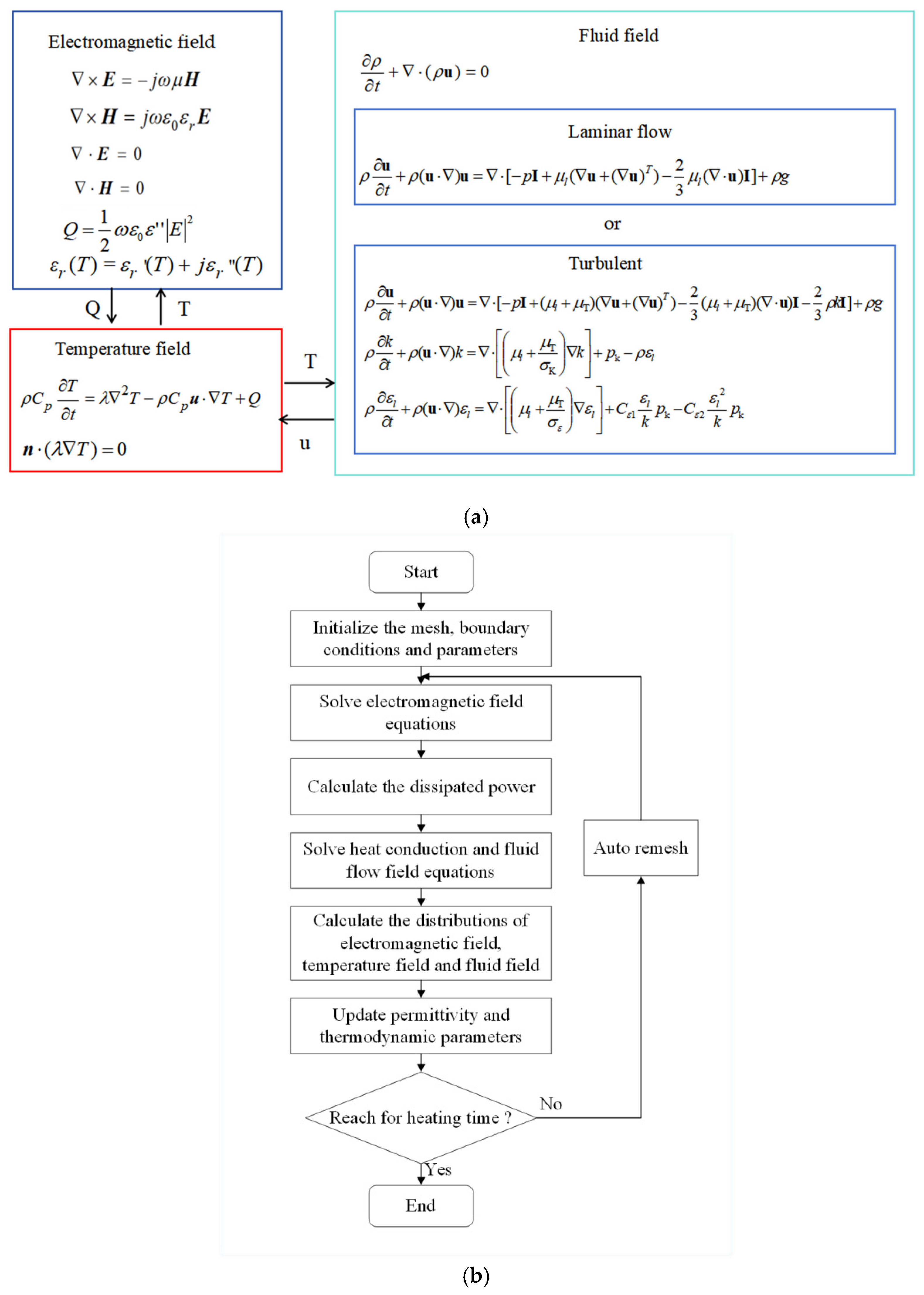
2.1.2. Analysis of Electromagnetic Field

The electromagnetic field distribution inside a microwave cavity can be described by Maxwell’s equations as follows:
× E = j ω μ H
× H = j ω ε 0 ε r E
E = 0
H = 0
where ω is the angular frequency of the electromagnetic wave, μ is the magnetic permeability, ε 0 is the permittivity in a vacuum, and ε r is the complex relative permittivity. The latter is defined as:
ε r = ε r + j ε r
where ε is the dielectric constant and ε is the dielectric loss factor. The complex relative permittivity can be described as a function of temperature:
  ε r ( T ) = ε r ( T ) + j ε r ( T )
where T is the real-time temperature and ε r T and ε r T are the real and imaginary parts of the relative permittivity of deionised water, respectively.
The metallic boundary is considered a perfect electric conductor and is defined as in [34]:
H n = 0 ,   E t = 0
where H n is the normal component of the magnetic field and E t is the tangential component of the electric field.

2.1.3. Analysis of Heat Transport

To simulate the complex heating process, the evaporation of water was ignored. The temperature field of the fluid was obtained by solving the heat conduction equation, which is expressed as follows:
ρ C p T t = λ 2 T ρ C p u T + Q
where C p is the thermal capacity at constant pressure, T is the temperature of the deionised water, λ is the heat conductivity coefficient, and Q is the energy absorbed from the microwave radiation, which can be expressed as follows:
Q = 1 2 ω ε 0 ε r | E | 2
The surface of the deionised water was set as a thermal insulation boundary, which is expressed as in [34]:
n ( λ T ) = 0
where n is the unit normal vector.

2.1.4. Analysis of Fluid Dynamics

Deionised water is considered compressible, which means that its physical properties, such as density ρ and dynamic viscosity μ l , are determined by the temperature. The Reynolds number of the fluid must be computed before an appropriate numerical model can be applied because it determines the state of the fluid flow. The Reynolds number of a liquid heated while using a rotating turntable or stirring paddle was calculated via the following:
R e ϕ = 2 π ρ N r 2 μ l
R e = ρ N D 2 μ l
where N represents the rotational and stirring frequencies of the turntable and paddle, respectively; r is the radius of the beaker; and D is the diameter of the paddle.
The Reynolds number is typically used to measure the state of motion in fluid dynamics calculations. Generally, laminar flow is dominant when the Reynolds number is lower than 2300, and k - ε turbulent flow is dominant when the Reynolds number is higher than 4000. The fluid is in a transitional region when the Reynolds number is between 2300 and 4000. In this study, the Reynolds numbers were 2538, 5077, and 7616 when the rotational frequencies were 10, 20, and 30 rpm, respectively. Therefore, the laminar model was used when the rotational frequency of the paddle was 10 rpm, whereas the k - ε turbulent model was used when the rotational frequencies were 20 and 30 rpm. The laminar flow model was applied to the water heated with a stirring paddle, as the maximum Reynolds number was 2254 when the stirring frequency was at the maximum of 30 rpm.
In the fluid flow model, mass conservation is controlled by the following continuity equation:
ρ t + ( ρ u ) = 0
The laminar flow model is described by the Navier-Stokes equation, which is expressed as follows:
ρ u t + ρ ( u ) u = [ p I + μ l ( u + ( u ) T ) 2 3 μ l ( u ) I ] + ρ g
where g is the acceleration due to gravity and I is the unit tensor.
The k - ε turbulence model incorporates two extra transport equations as well as two dependant variables, the turbulent kinetic energy k and dissipation rate ε l . The viscosity in the k - ε turbulence model includes a turbulent viscosity term μ T . Thus, the momentum conservation equation is expressed as in [35]:
ρ u t + ρ ( u ) u = [ p I + ( μ l + μ T ) ( u + ( u ) T ) ] 2 3 [ ( μ l + μ T ) ( u ) I + ρ k I ] + ρ g
and the turbulent viscosity μ T is modelled as follows:
μ T = ρ C μ k 2 ε l
where C μ is a constant.
The transport equation for k is described as follows:
ρ k t + ρ ( u ) k = μ l + μ T σ K k + p k ρ ε l
where the production term p k is defined as follows:
p k = μ T u : ( u + ( u ) T ) 2 3 ( u ) 2 2 3 ρ k u
The transport equation for ε l is described as follows:
ρ ε l t + ρ ( u ) ε l = μ l + μ T σ ε ε l + C ε 1 ε l k p k C ε 2 ε l 2 k p k
The empirical coefficients of the k - ε model are C ε 1 = 1.44 , C ε 2 = 1.92 , C μ = 0.09 , σ k = 1 , and σ ε = 1.3 .
The wall of the beaker was set as a no-slip wall, which implied that the velocity was u = 0 . The surface of the paddle was set as a moving wall, and its movement was described by the following:
u x = d x d t , u y = d y d t , u z = 0
where ux, uy, and u z are the components of the velocity along the x, y, and z-directions, respectively.
The boundary condition at the dividing surface between the deionised water and the air was set as the symmetry boundary, which was governed by [35]:
u × n = 0
where n is the unit normal vector of the velocity.

2.1.5. Analysis of the ALE Method

For modelling the microwave heating with a stirring paddle, the ALE method was used to capture the boundary changes caused by the stirring paddle. The ALE method is a numerical simulation technique that combines the advantages of the Lagrangian and Euler methods. It establishes a mesh coordinate system that includes a mesh and a spatial coordinate system. Using a specific mapping between these two coordinate systems, the physical quantities of the nodes in the mesh coordinate system can be projected onto the corresponding nodes in the spatial coordinate system [35]. To investigate the microwave heating of the fluid when it is stirred, the electromagnetic field distribution was modelled using the Eulerian method, and the velocity and temperature distributions were modelled using the Lagrangian method. Thus, at each time step, the ALE method considered not only the motion characteristics of the fluid but also the deformation of the computational mesh of the paddle, enabling the interaction between the fluid and solid boundaries to be captured more accurately. In a previous study [34], the ALE method was validated as suitable for modelling microwave heating and more efficient than the conventional method, which needs to divide the whole heating time into multiple sections and uses the solution of the previous moment as the initial value for calculating the next moment through programming. However, the mesh needs to be updated, as the boundary of the anchor paddle is time-dependent. The area inside the deionised water was set as a rotating domain, which was described by the coordinate transformations as follows:
d x = X c o s 2 π f t Y sin 2 π f t X d y = Y c o s 2 π f t + X sin 2 π f t Y d z = 0
where x and y are the coordinates in the spatial frame and X and Y are the coordinates in the material frame. Other areas in the oven were set as free deformation domains, which allowed the mesh elements to adapt to the deformation caused by the stirring and rotation. The configuration described above is also applicable to the method of rotating the turntable.

2.1.6. Input Parameters

The thermo-physical properties of the deionized water are presented in Table 1. The real part εr′(T) = 85.9 − 0.36 × T − 2.44 × 10⁻⁵ × T2 + 6 × 10⁻⁶ × T3 and the imaginary part εr″(T) = 19.42 − 0.55 × T + 0.01 × T2 − 2.61 × 10⁻⁵ × T3 of the relative permittivity of deionized water were measured by the Agilent E5071C ENA Network Analyzer.

2.1.7. Multi-Physics Fields Coupling Calculation

The calculations for the coupling of the multi-physics field is shown in Figure 2a. Because the permittivity depends on the temperature, the distribution of the electromagnetic field in the deionised water is determined by Maxwell’s equations, and the initial dielectric properties corresponding to T0 = 30 °C and the dissipated power Q are decided by the initial dielectric properties and the electric field above, respectively. The new temperature T was dictated by tackling the fluid dynamics and heat conduction equations after the dissipated power Q was introduced into the heat conduction equation. The permittivity was then updated according to the new temperature, after which it was used to recalculate the electromagnetic fields. Thermodynamic parameters such as the density ρ , dynamic viscosity μ l , heat capacity at constant pressure C p , and heat conductivity coefficient k were also updated to compute the velocity and temperature distributions. An iterative flow diagram of the multi-physics field calculations is shown in Figure 2b.
To calculate the transient field solution for the three physical fields, COMSOL 5.3a software and a workstation with a 16 core CPU (Intel Xeon Gold 6248R) and 64 GB RAM were used. The entire solution domain was divided into 85,700 elements, for which the mesh element quality was greater than 0.24. The solution domain of the paddle was divided using a maximum element size smaller than 2 mm. The simulation of the time-dependent heating process lasting 90 s took 72 h.

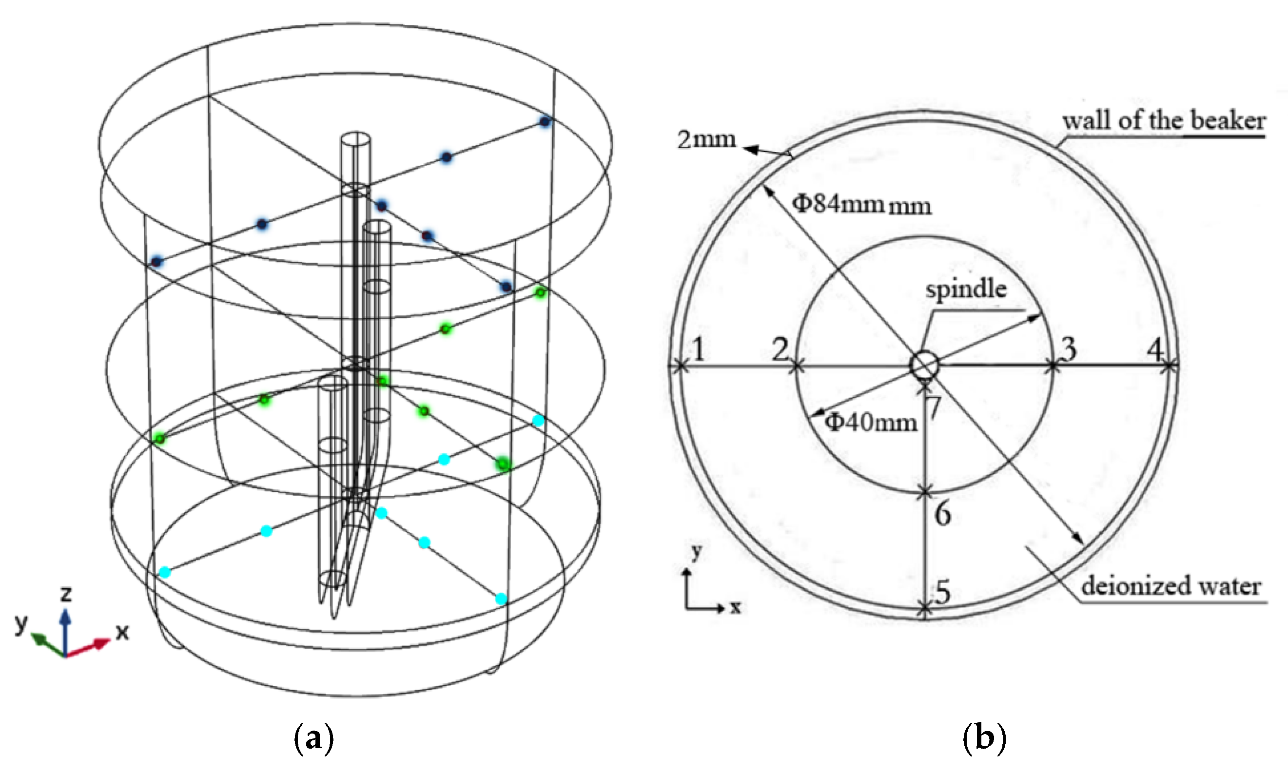
2.2. Experimental Setup

The temperature of the water was measured with a UMI-8 optical fibre thermometer with an accuracy of 0.05 °C. The temperatures measured at different locations are shown in Figure 3a. To comprehensively probe the volumetric temperature distribution, seven points in each of three horizontal layers, which were positioned at heights of 16.5, 45, and 80 mm from the bottom of the beaker (and denoted as the low, middle, and high planes, respectively), were measured. The points to be measured in each layer were marked with numbers ranging from 1 to 7, as shown in Figure 3b. Points 1, 4, and 5 were positioned 2 mm from the beaker wall and 42 mm from the centre of the beaker. Points 2, 3, and 6 were located 20 mm from the centre of the beaker. Finally, point 7 was located 7.5 mm from the centre of the circle. Three points were measured along the y-axis because the temperature distribution was approximately symmetrical along the x-o-z plane owing to the same symmetry in the geometry of the oven.
To ensure the repeatability of the measurements, the beaker with the stirring paddle located in the centre was placed in a fixed position marked on the tray, and the probe passing through seven holes on the upper shell of the microwave oven was fixed with a customised clamping bracket to mark the locations of the points in the beaker to be measured. For all experiments, the initial temperatures of the water and laboratory were the same, the seven points in each horizontal plane were measured simultaneously, and the temperature of each plane was measured 10 times.

3. Results and Discussion

3.1. Experimental Validation

To prove the validity of the calculated model, an experiment was designed to measure the temperature of the deionised water at the points shown in Figure 3. The calculated and measured results for the spatial points shown in Figure 3 with a rotating turntable and stirring paddle are depicted in Table 2 and Table 3, respectively. The errors in the measured results were calculated using measurements performed several times [36]. As indicated in Table 2 and Table 3, the simulated results roughly agreed with the measured values, and the maximum differences between the calculated and measured temperatures were ΔTAamax = (6.94 ± 0.068) °C ((TA7 − Ta7)|20rpm = 48.2 °C − (41.26 °C ± 0.068 °C)) and ΔTBbmax = (6.3 ± 0.045) °C ((TB7 − Tb7)|20rpm = 53.3 °C − (47.0 °C ± 0.045 °C)) for the rotation and stirring methods, respectively. The differences between the calculated and measured temperatures primarily arose from the simplification of the simulation model relative to the actual situation and the measurement error. In the simulation, the evaporation of the deionised water, which removed heat and mass simultaneously, was ignored, and the boundary conditions of the beaker wall and bottom were assumed to be adiabatic (i.e., the heat transfer from the beaker to the air and tray was neglected). During the measurements, the errors originated from the precision of the probe of the temperature sensor (±0.05 °C) and its limited spatial resolution (2 mm in diameter). However, in the simulation, the temperature measurement points were approximated as infinitesimal points without volume, and the rise in the temperature of the deionised water in the microwave cavity was caused by the thermal convection from the air to the deionised water.
As indicated in Table 2, the maximum temperature differences between the calculated and measured results for the seven points in every horizontal plane were ΔTXxmax = 4.3 °C ((TB7 − TB1)|30rpm = 52.3 °C − 48.0 °C) and ΔTxxmax = (3.8 ± 0.116) °C ((Tb2 − Tb5)|30rpm = (48.58 ± 0.058) °C − (44.78 ± 0.058) °C). However, along the vertical plane, the temperature differences ΔTAC and ΔTac were almost more than 10 °C, and the minimum values for the calculated and measured results were ΔTAcmin = 8.8 °C ((TC6 − TA6)|30rpm = 56.7 °C − 47.9 °C) and ΔTacmin = (12.46 ± 0.124) °C ((Tc4 − Ta4)|30rpm = (55.88 ± 0.058) °C − (43.42 ± 0.066) °C), respectively, which indicated that the non-uniformity existed primarily along the vertical plane of the deionised water. In addition, the temperature differences between the calculated and measured results along the vertical plane changed slightly as the rotational frequency increased from 10 to 30 rpm, demonstrating that the temperature differences were difficult to eliminate by increasing the rotational frequency.
As indicated in Table 3, among the seven points in every horizontal plane, the maximum temperature difference of the calculated results ΔTXxmax = 3.3 °C ((TB7 − TB5)|20rpm = 53.3 °C − 50.0 °C) and that of the measured values ΔTxxmax = (1.86 ± 0.083) °C ((Tc6 − Tc1)|20rpm = (53.4 ± 0.032) °C − (51.54 ± 0.051) °C) were smaller than the values of 4.3 °C and 3.8 °C for the rotating turntable mentioned above. This means that the temperature in the horizontal plane of the water heated by the stirring paddle was more uniform than that of the rotation method. Furthermore, after increasing the stirring frequency from 10 to 20 rpm, the maximum temperature differences along the vertical plane between the calculated and measured results decreased from ΔTAcmax = 13.9 °C ((TC7 − TA7)|10rpm = 58.9 °C – 45 °C) and ΔTacmax = (13.54 ± 0.122) °C ((Tc5 − Ta5)|10rpm = (57.34 ± 0.051) °C − (43.80 ± 0.071) °C to ΔTAcmax = 5.7 °C ((TC7 − TA7)|20rpm = 53.3 °C − 47.6 °C) and ΔTacmax = (7.58 ± 0.081) °C ((Tc6 − Ta6)|20rpm = (53.4 ± 0.032) °C − (45.82 ± 0.049) °C). As the stirring frequency increased to 30 rpm, the maximum temperature differences between the calculated and measured results decreased to ΔTAcmax = 2.8 °C ((TC7 − TA7)|30rpm = 51.7 °C − 48.9 °C) and ΔTacmax = (1.64 ± 0.145) °C ((Tc7 − Ta7)|30rpm = (49.98 ± 0.058) °C − (48.34 ± 0.087) °C), and the minimum temperature differences between the calculated and measured results were only ΔTAcmin = 0.7 °C ((TC1 − TA1)|30rpm = 50.5 °C − 49.8 °C) and ΔTacmin = (0.52 ± 0.129) °C ((Tc1 − Ta1)|30rpm = (49.62 ± 0.058) °C − (49.10 ± 0.071) °C). Thus, the uniformity along the vertical plane of the microwave heating improved substantially as the stirring frequency increased. As a result, stirring was more effective than rotation in eliminating the non-uniformity of the microwave heating.

3.2. Theoretical Calculation

To compare the uniformity of the microwave heating corresponding to the stirring and traditional rotation methods, this section discusses the electromagnetic, temperature, and velocity fields.

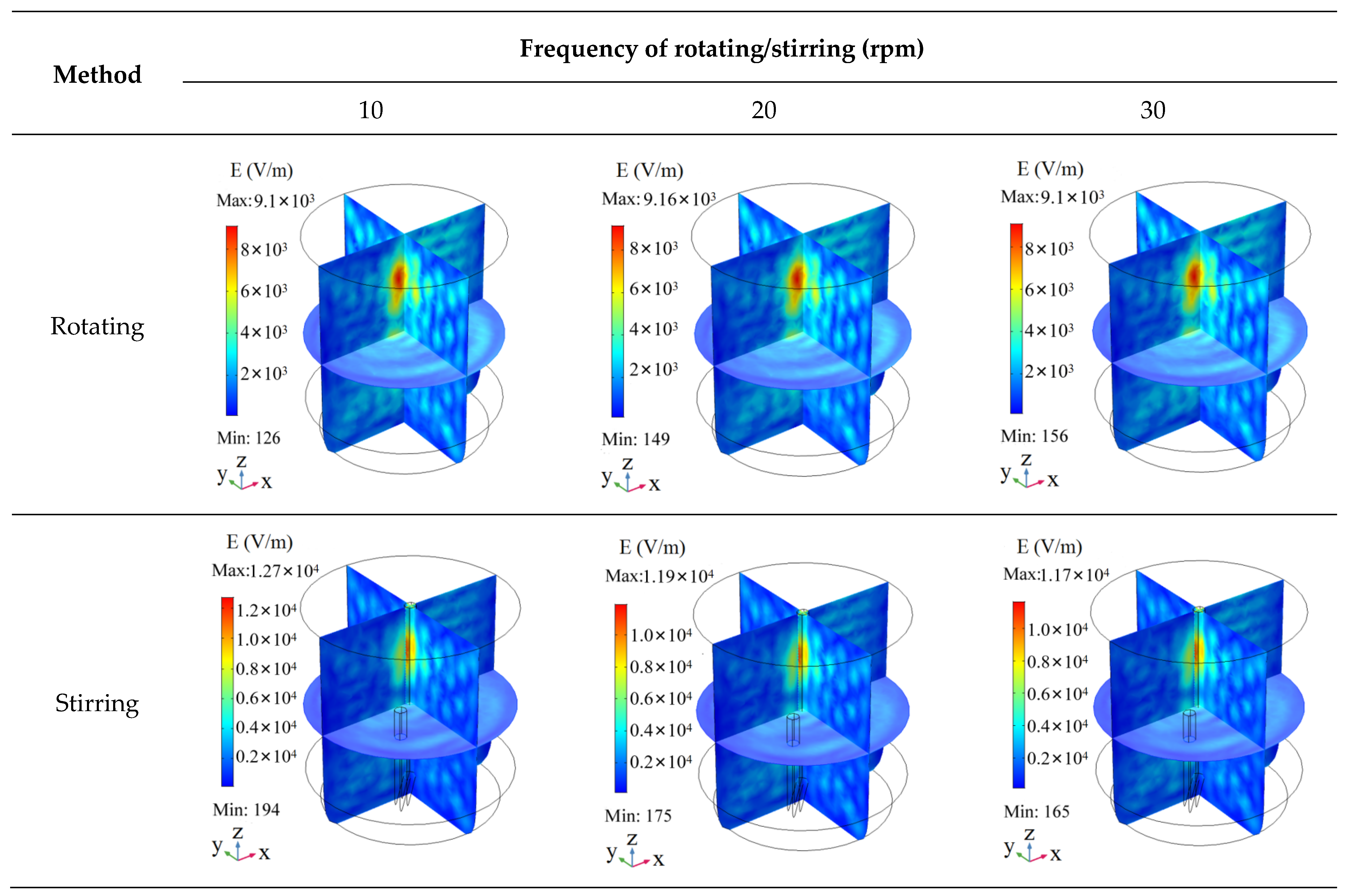
3.2.1. Analysis of Electric Field

The distributions of the electric field inside the deionised water for the rotation and stirring methods are shown in Figure 4. The electric field intensity inside the deionised water was not uniform at different rotation and stirring frequencies. A region in which the electric field was high existed in the centre near the upper surface of the water, indicating that a hotspot could exist in the temperature field at the same position. Moreover, the maximum electric field intensity decreased as the rotational and stirring frequency increased, whereas the minimum electric field intensity exhibited the same trend as the frequency. This can be attributed to the fact that the temperature-dependent permittivity used for calculating the electric field distribution varied with the rotational and stirring frequency. These slight variations in the maximum and minimum electric field intensities caused by the increase in the rotational and stirring frequencies show that the proposed simulation method can account for the interactions between electromagnetic waves and the temperature.

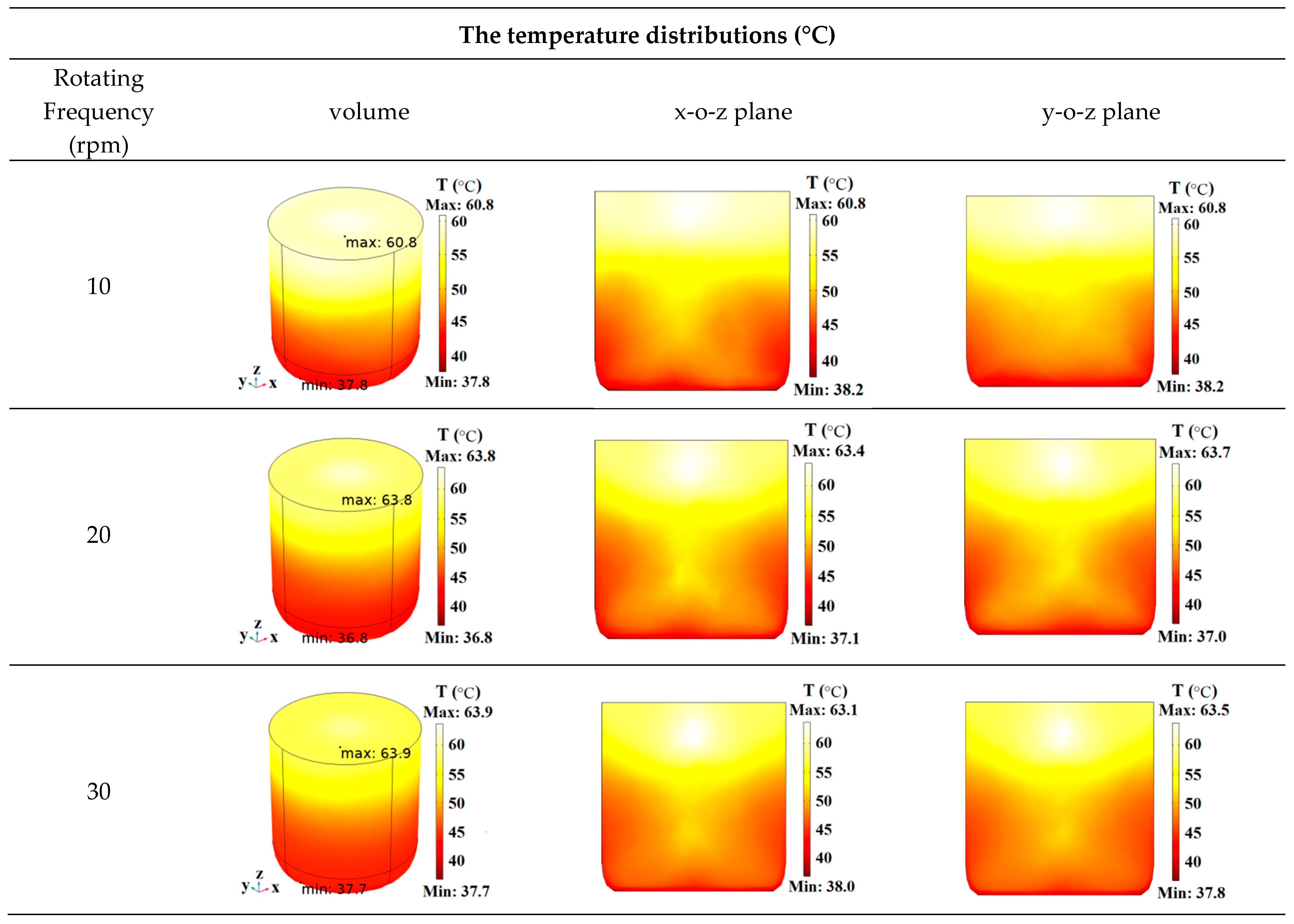
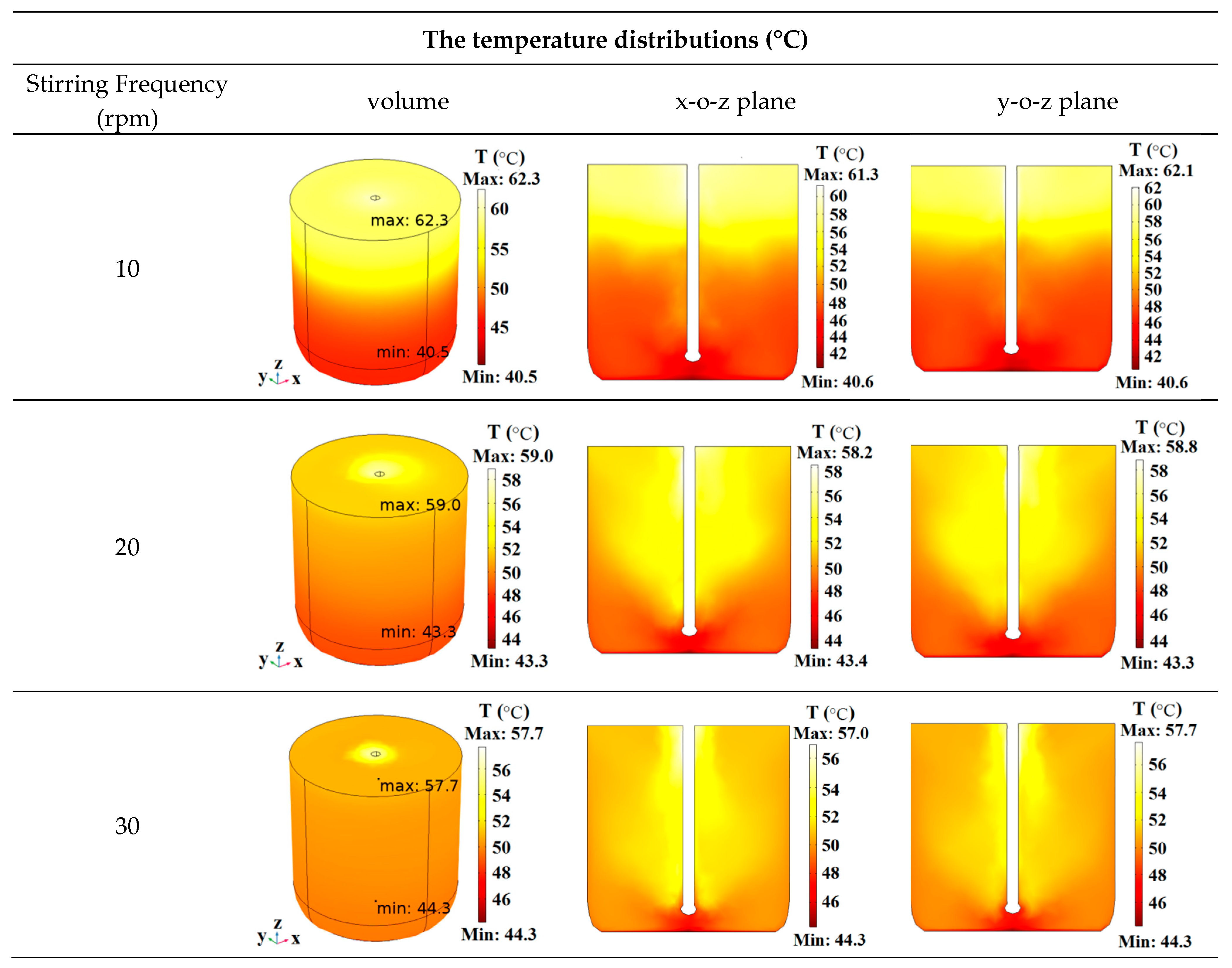
3.2.2. Analysis of the Temperature Field

To comprehensively probe the heating uniformity, the temperature distributions in the deionised water for the turntable rotation and stirring paddle methods are shown in Figure 5 and Figure 6, respectively. According to the figures, the temperature distributions in the horizontal plane were uniform, although the temperature in the central area of the horizontal plane was higher than that near the wall of the beaker. The non-uniformity in the horizontal plane can be attributed to the centrifugal force, which caused water with a lower temperature to flow away from the centre of the beaker.
As indicated in Figure 5, the temperature in the upper area was higher than that near the bottom. At the same time, the maximum and minimum temperatures appeared near the surface and bottom, respectively, indicating that the temperature gradient was primarily along the vertical direction. This characteristic of the temperature distribution, particularly the location of the spot with the highest temperature, exhibited a strong correlation with the electric field distribution, which is shown in Figure 4. In addition to the contribution of the electric field, the temperature distribution was also influenced by natural convection, which transferred the high-temperature fluid with a lower density to the upper region and the low-temperature fluid with a higher density to the bottom. A comparison between the results for different rotational frequencies showed that the temperature difference ΔT = Tmax − Tmin increased from 23.0 °C (60.8 − 37.8 °C) to 27 °C (63.8 − 36.8 °C) and then decreased to 26.2 °C (63.9 − 37.7 °C) when the rotational frequency increased from 10 rpm to 20 and 30 rpm, indicating that the traditional method of turntable rotation made a small contribution to improving the heating uniformity along the vertical plane.
As indicated in Figure 6, the temperature in the upper region was higher than that in the lower region when the stirring frequency of the paddle was 10 rpm. Nevertheless, the boundary between the high- and low-temperature regions became obscure when the stirring frequency was gradually increased to 20 and 30 rpm. The maximum temperature difference ΔT = Tmax − Tmin sharply declined from 21.8 °C (62.3 − 40.5 °C) to 13.4 °C (57.7 − 44.3 °C) as the stirring frequency increased from 10 to 30 rpm, indicating that the temperature gradient had been decreased effectively. Comparing Figure 5 and Figure 6, the temperature profile along the vertical plane for the water heated with the stirring paddle was more uniform than that of the rotation method for the same frequency. This indicated that the proposed method (using an anchor paddle) was more effective at enhancing the uniformity of the microwave heating than the traditional method of rotating the turntable.

3.2.3. COV of the Temperature

The coefficient of variation (COV), which is the ratio of the standard deviation to the mean, can effectively remove the effect of the mean on the standard deviation. It is widely used to quantify heating non-uniformities [37]. A smaller COV value indicates a higher degree of heating uniformity and vice versa. The COV of the temperature of a given volume is computed via the following:
C O V = σ ( T ) E ( Δ T ) = 1 V ( T i E ( T ) ) 2 Δ ν i E ( Δ T )
where T i is the temperature of the i-th volumetric element, Δ v i is the volume of the i-th element,   E ( T ) is the average temperature increment, and   E ( Δ T ) is the mean temperature.
The calculated results for the temperature COV of the deionised water are listed in Table 4. The temperature COV of the water heated with the rotating turntable was 22.3%, 22.3%, and 19.5% under rotational frequencies of 10, 20, and 30 rpm, respectively, indicating that the temperature uniformity underwent almost no changes. In contrast, the temperature COV of the water heated by the stirring method was 19.8%, 7.5%, and 3.6% for stirring frequencies of 10, 20, and 30 rpm, respectively, indicating that the temperature uniformity in the water was enhanced as the frequency increased.
Compared to the traditional method of rotating the turntable, the temperature uniformity of the water heated with the stirring paddle improved by 11.2% ((22.3 − 19.8)/22.3%), 66.4% ((22.3 − 7.5)/22.3) and 81.5% ((19.5 − 3.6%)/19.5%) when the rotational and stirring frequencies were 10, 20, and 30 rpm, respectively. Therefore, stirring is more effective for improving the uniformity along the vertical plane of microwave-heated fluids.

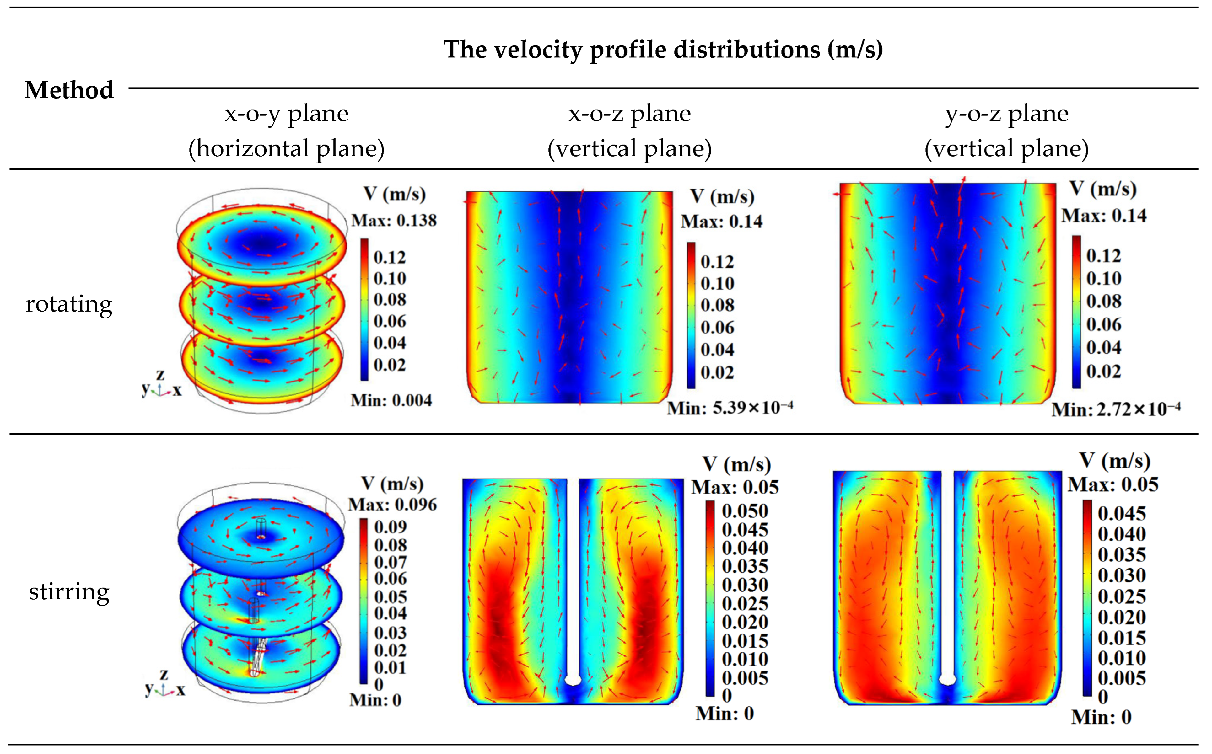
3.2.4. Analysis of the Velocity Field

The velocity field distributions of the deionised water heated with a rotating turntable and stirring paddle for a rotational and stirring frequency of 30 rpm are exhibited in Figure 7. The red arrows in Figure 7 represent the velocity directions of the fluid particles. According to the panels in the first row, the velocity of the fluid particles, particularly those near the wall of the beaker, were approximately tangential to the circle in the x-o-y horizontal plane, although a few vertical components in the x-o-z and y-o-z vertical planes existed. This means that the method of rotating the turntable did not significantly enhance the upward and downward flow of the fluids to enhance the convective heat transfer and eliminate the vertical temperature difference. According to the panels in the second row, the velocity of the fluid particles heated with the stirring paddle had large vertical components in the x-o-z and y-o-z vertical planes, with a maximum speed of 0.05 m/s. In other words, the forced convention caused by the stirring enhanced the axial fluid flow, which enabled the heat transfer to decrease the vertical temperature difference. The velocity field distributions explain the influence of the rotation and stirring on the temperature distributions, which are shown in Figure 5 and Figure 6. In summary, stirring using an anchor paddle can effectively eliminate vertical temperature non-uniformity and generate more uniform heating.

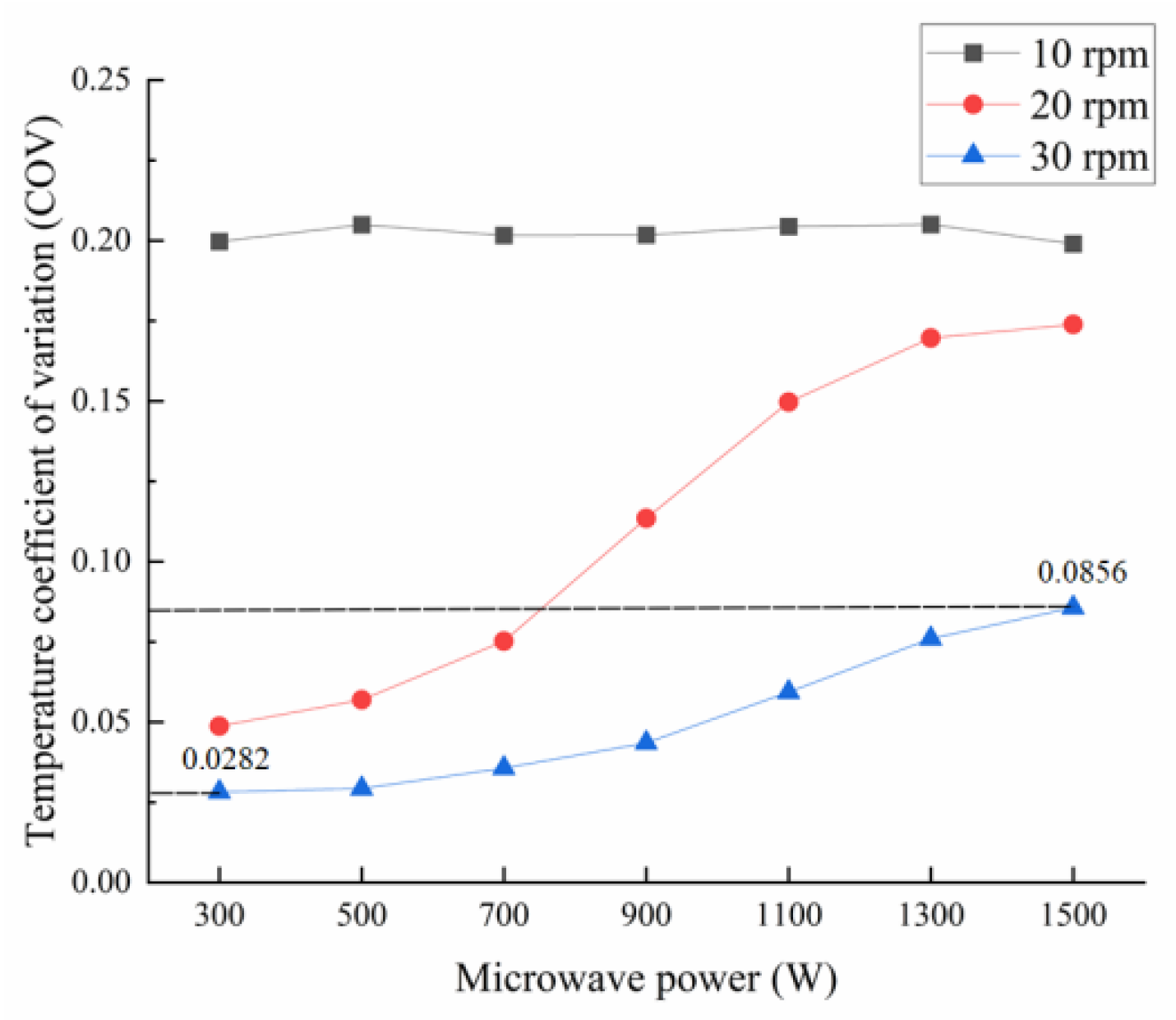
3.2.5. Analysis of the Effect of Microwave Power on Temperature COV with Stirring

To understand the effect of the microwave power on the COV of the temperature under symmetrical stirring, the COV of the deionised water is shown in Figure 8. The COV slightly fluctuated around 0.2 when the stirring frequency was 10 rpm, indicating that the input power had a minimal effect on the heating uniformity of the stirred water. When the stirring frequency was 20 and 30 rpm, the COV increased as the power increased, but the magnitude was significantly slowing down. In particular, when the stirring frequency was 30 rpm, the COV was significantly smaller than that at 10 rpm and 20 rpm as the input power rose from 300 W to 1500 W, and it remained at a low level of less than 0.09, indicating that stirring effectively enhanced the heating uniformity.
Overall, the heating uniformity is significantly improved because the proposed mixed-flow agitator of the anchor paddle enhances the forced convection of the fluid to reduce the temperature difference induced along the vertical direction by a non-uniform electric field and natural convection. However, the mechanical complexity and energy consumption, along with the agitator, may be drawbacks of the stirring method. These costs may be worthwhile considering the potential economic benefits of uniform heating. Therefore, more economical and effective methods will be worth investigating in future studies.

4. Conclusions

In this study, a three-dimensional model that solves the coupled Maxwell equations, heat conduction equation, and fluid flow equations was combined with the ALE method to assess the improvement in the temperature uniformity of a microwave-heated fluid undergoing symmetrical stirring by an anchor paddle. The temperature distributions of the deionised water subjected to microwave heating plus stirring or turntable rotation were compared, and the results were validated experimentally. The electric, temperature, and velocity fields in the heated water that underwent stirring were analysed for different stirring frequencies, and the results were compared to those corresponding to the rotating turntable. The conclusions are as follows.
  • The coincidence between the experimental and calculated results demonstrated that the proposed FEM multi-physics calculation model is capable of predicting the temperature of a fluid subjected to microwave heating with stirring.
  • The non-uniform temperature distribution of the water heated with the rotating turntable was primarily concentrated along the vertical plane, and the rotation had a very minimal effect on reducing the temperature difference. This characteristic of the temperature distribution was the result of the combined effect of the non-uniform electric field distribution and natural convection. In contrast, the temperature uniformity of the water heated with stirring improved because the forced convection enhanced the vertical flow of the fluid and effectively eliminated the vertical temperature difference. For the same rotational/stirring frequency, the COV of the water heated with a stirring paddle improved by 11.2–81.5% compared to that heated with rotation.
These results demonstrated that stirring with an anchor paddle was a more effective approach for improving the microwave heating uniformity of the fluid than the traditional method of rotating the turntable because stirring decreased the vertical temperature difference along the vertical axis of the fluid.
Future studies should focus on additional aspects to improve the uniformity of microwave heating. In terms of improving the electric field distribution, designing special waveguides and cavities; optimising their shape, size, and location; adding more waveguides; and utilising mode stirrers should be considered. In terms of enhancing the heat transfer, optimising the shape, size, and location of the paddle in the heated fluid may be more effective. Furthermore, combining the proposed method with other volumetric heating methods, such as ultrasonic heating, may also be potentially advantageous. From the view of scaling up the stirring method for industrial applications, the stirring method may encounter potential challenges, such as the coordinated control mechanism for energy coupling between the microwave field and mechanical stirring; the issue of stirring efficiency and equipment adaptability; the problem of stirring paddle material compatibility and long-term operational reliability; and the challenge of inline monitoring of temperature uniformity in continuous production. These studies will be helpful in providing effective solutions for microwave heating systems.

Author Contributions

W.T. developed the model and analysed the data; W.T., X.F., L.G., K.C. and Y.C. wrote the initial draft of the manuscript; W.T., J.S. and H.L. reviewed and contributed to the final manuscript. All authors have read and agreed to the published version of the manuscript.

Funding

This research was funded by the Science and Technology Cooperation and Exchange Special Project of Shanxi Province (202204041101030) and the Scientific and Technological Achievements Transformation and Guidance Project of Shanxi Province (202304021301044).

Data Availability Statement

The original contributions presented in the study are included in the article; further inquiries can be directed to the corresponding author.

Conflicts of Interest

The authors declare no conflicts of interest.

References

  1. Delouei, A.A.; Naeimi, H.; Sajjadi, H. An active approach to heat transfer enhancement in indirect heaters of city gate stations: An experimental modeling. Appl. Therm. Eng. 2024, 237, 121795–121806. [Google Scholar] [CrossRef]
  2. Hedeshi, M.; Jalali, A.; Arabkoohsar, A.; Amiri Delouei, A. Nanofluid as the working fluid of an ultrasonic-assisted double-pipe counter-flow heat exchanger. J. Therm. Anal. Calorim. 2023, 148, 8579–8591. [Google Scholar] [CrossRef]
  3. Hashemi, S.M.B.; Akbari, M.; Roohi, R.; Phimolsiripol, Y. Hurdle approaches using conventional thermal, microwave heating and ginger essential oil in vegetable juice mixture: Heat transfer modeling and microbial inactivation kinetics. LWT-Food Sci. Technol. 2024, 198, 115958–115967. [Google Scholar] [CrossRef]
  4. Jiao, X.; Diao, H.; Liu, T.; Yan, B.; Tang, X.; Fan, D. Single-mode microwave heating for food science research: Understanding specific microwave effects and reliability concerns. Food Phys. 2025, 2, 100048–100060. [Google Scholar] [CrossRef]
  5. Lee, Y.-C.; Hwang, C.-C.; Tsai, Y.-H.; Huang, Y.-T. Development and pasteurization of in-packaged ready-to-eat rice products prepared with novel microwave-assisted induction heating (MAIH) technology. Appl. Food Res. 2025, 5, 100697–100706. [Google Scholar] [CrossRef]
  6. Li, G.; Zhou, J. COMSOL-Based Simulation of Microwave Heating of Al2O3/SiC Composites with Parameter Variations. Symmetry 2024, 16, 1254. [Google Scholar] [CrossRef]
  7. Zhang, P.; Liang, C.; Chen, X.; Liu, D.; Ma, J. Insight into microwave heating patterns for sustainable decomposition of plastic wastes into hydrogen. Appl. Therm. Eng. 2025, 260, 124954–124966. [Google Scholar] [CrossRef]
  8. Zhang, S.; Qin, S.; Wan, W.; Li, J.; Liu, S.; Paik, K.-W.; He, P.; Zhang, S. Investigation on electromagnetic and heat transfer coupling of heating susceptor for selective microwave hybrid soldering: 3D multi-physics simulation and experiment. Appl. Therm. Eng. 2024, 255, 124047–124060. [Google Scholar] [CrossRef]
  9. Principato, L.; Spigno, G. Chapter 16—Microwave heating in food processing. In Food Packaging and Preservation; Jaiswal, A.K., Shankar, S., Eds.; Academic Press: Cambridge, MA, USA, 2024; pp. 299–329. [Google Scholar]
  10. Taguchi, Y.; Abea, A.; Llave, Y.; Sugihara, C.; Suzuki, F.; Hosoda, T.; Onizawa, K.; Sakai, N.; Fukuoka, M. Modeling of microwave thawing and reheating of multiphase foods: A case study for packed rice. J. Food Eng. 2025, 386, 112284–112294. [Google Scholar] [CrossRef]
  11. Yi, M.; Tang, X.; Liang, S.; He, R.; Huang, T.; Lin, Q.; Zhang, R. Effect of microwave alone and microwave-assisted modification on the physicochemical properties of starch and its application in food. Food Chem. 2024, 446, 138841–138853. [Google Scholar] [CrossRef]
  12. Chen, W.-H.; Liu, L.-X.; Khoo, K.S.; Sheen, H.-K.; Kwon, E.E.; Saravanakumar, A.; Chang, J.-S. Environmentally-friendly alkaline ionized water pretreatment and hydrolysis of macroalga via microwave-assisted heating to improve monosaccharide yield for bioethanol production. Process Saf. Environ. Prot. 2024, 189, 702–713. [Google Scholar] [CrossRef]
  13. Han, Y.; Meng, L.-Y.; Lin, R.; Kim, S.; Kim, T.; Wang, X.-Y. Evaluating the sustainability of microwave pre-cured high-volume slag concrete: Mechanical properties, environmental impact and cost-benefit analysis. J. Build. Eng. 2024, 96, 110663–110684. [Google Scholar] [CrossRef]
  14. Zhang, C.; Chen, W.-H.; Ho, S.-H. Economic feasibility analysis and environmental impact assessment for the comparison of conventional and microwave torrefaction of spent coffee grounds. Biomass Bioenergy 2023, 168, 106652–106664. [Google Scholar] [CrossRef]
  15. Ahmad, F.; Zhang, Y.; Fu, W.; Zhao, W.; Xiong, Q.; Li, B. Microwave-assisted chemical looping gasification of sugarcane bagasse biomass using Fe3O4 as oxygen carrier for H2/CO-rich syngas production. Chem. Eng. J. 2024, 501, 157675–157687. [Google Scholar] [CrossRef]
  16. Fu, W.; Zhang, Y.; Cao, W.; Zhao, W.; Li, B. Microwave-assisted chemical looping gasification of plastics for H2-rich gas production. Chem. Eng. J. 2024, 499, 156225–156236. [Google Scholar] [CrossRef]
  17. Khodabandehloo, M.; Shabanian, J.; Harvey, J.-P.; Chaouki, J. Kinetic study of microwave heating-assisted chemical looping dry reforming of methane over magnetite. Int. J. Hydrogen Energy 2024, 96, 1079–1086. [Google Scholar] [CrossRef]
  18. Liu, J.; Li, H.; Liu, Z.; Meng, X.; He, Y.; Zhang, Z. Study on the process of medical waste disinfection by microwave technology. Waste Manag. 2022, 150, 13–19. [Google Scholar] [CrossRef]
  19. Vadivambal, R.; Jayas, D.S. Non-uniform temperature distribution during microwave heating of food materials—A review. Food Bioprocess Technol. 2010, 3, 161–171. [Google Scholar] [CrossRef]
  20. Karlsson, M.; Carlsson, H.; Idebro, M. Microwave heating as a method to improve sanitation of sewage sludge in wastewater plants. IEEE Access 2019, 7, 142308–142316. [Google Scholar] [CrossRef]
  21. Horikoshi, S.; Serpone, N. Microwave flow chemistry as a methodology in organic syntheses, enzymatic reactions, and nanoparticle syntheses. Chem. Rec. 2019, 19, 118–139. [Google Scholar] [CrossRef]
  22. Alzubaidi, S.; Wallace, A.; Naidu, S. Single-arm prospective study comparing ablation zone volume between time zero and 24 h after microwave ablation of liver tumors. Abdom. Radiol. 2024, 49, 3136–3142. [Google Scholar] [CrossRef] [PubMed]
  23. Manickavasagan, A.; Jayas, D.S.; White, N.D.G. Non-uniformity of surface temperatures of grain after microwave treatment in an industrial microwave dryer. Drying Technol. 2006, 24, 1559–1567. [Google Scholar] [CrossRef]
  24. Baro, R.K.; Kotecha, P.; Anandalakshmi, R. Optimization of continuous-flow microwave processing with static mixers for enhanced heating uniformity. Food Bioprod. Process. 2025, 149, 401–414. [Google Scholar] [CrossRef]
  25. Wang, C.; Peng, Z.; Yang, F.; Zhu, H.; Yan, L. Uniformity improvement of microwave heating with switchable frequency selective surface. Case Stud. Therm. Eng. 2024, 61, 104919–104928. [Google Scholar] [CrossRef]
  26. Zhu, H.; He, J.; Hong, T.; Yang, Q.; Wu, Y.; Yang, Y.; Huang, K. A rotary radiation structure for microwave heating uniformity improvement. Appl. Therm. Eng. 2018, 141, 648–658. [Google Scholar] [CrossRef]
  27. Zhu, J.; Li, F.; Wang, H.; Yang, Z.; Chen, H.; Zhu, H. Numerical analysis of microwave-enhanced oil shale pyrolysis by rotation turntable based on the Arbitrary Lagrangian-Eulerian method. Fuel 2024, 371, 131925–131937. [Google Scholar] [CrossRef]
  28. Wang, L.; Kang, J.; Zhu, C.; Zhou, Z.; Wang, S.; Huang, Z. Modeling the RF heating uniformity contributed by a rotating turntable. J. Food Eng. 2023, 339, 111289–111302. [Google Scholar] [CrossRef]
  29. Yang, R.; Chen, J. Identification of turntable function in a solid-state microwave heating process with diverse frequency-shifting strategies applied. Innov. Food Sci. Emerg. Technol. 2024, 94, 103670–103682. [Google Scholar] [CrossRef]
  30. Shen, L.; Gao, M.; Feng, S.; Ma, W.; Zhang, Y.; Liu, C.; Liu, C.; Zheng, X. Analysis of heating uniformity considering microwave transmission in stacked bulk of granular materials on a turntable in microwave ovens. J. Food Eng. 2022, 319, 110903–110922. [Google Scholar] [CrossRef]
  31. Liu, M.; Zhou, D.; Peng, Y.; Tang, Z.; Huang, K.; Hong, T. High-efficiency continuous-flow microwave heating system based on metal-ring resonant structure. Innov. Food Sci. Emerg. Technol. 2023, 85, 103330–103343. [Google Scholar] [CrossRef]
  32. Yang, F.; Zhu, H.; Yang, Y.; Huang, K. High-Efficiency Continuous-Flow Microwave Heating System Based on Asymmetric Propagation Waveguide. IEEE Trans. Microw. Theory Tech. 2022, 70, 1920–1931. [Google Scholar] [CrossRef]
  33. Zhu, H.; Shu, W.; Xu, C.; Yang, Y.; Huang, K.; Ye, J. Novel electromagnetic-black-hole-based high-efficiency single-mode microwave liquid-phase food heating system. Innov. Food Sci. Emerg. Technol. 2022, 78, 103012–103021. [Google Scholar] [CrossRef]
  34. Zhou, J.; Yang, X.; Ye, J. Arbitrary Lagrangian-Eulerian method for computation of rotating target during microwave heating—ScienceDirect. Int. J. Heat Mass Transf. 2019, 134, 271–285. [Google Scholar] [CrossRef]
  35. Wilcox, D. Turbulence Models for CFD, 2nd ed.; DCW Industries, Inc.: La Canada, CA, USA, 1998. [Google Scholar]
  36. Taylor, J. An Introduction to Error Analysis; University Science Books: Mill Valley, CA, USA, 1982. [Google Scholar]
  37. Pitchai, K.; Chen, J.; Birla, S.; Gonzalez, R.; Jones, D.; Subbiah, J. A microwave heat transfer model for a rotating multi-component meal in a domestic oven: Development and validation. J. Food Eng. 2014, 128, 60–71. [Google Scholar] [CrossRef]
Figure 1. The calculation model of microwave heating of deionized water with the method of stirring by an anchor paddle used in this study. (a) 3D model; (b) x-o-z plane view.
Symmetry 17 00659 g001
Figure 2. A chart showing the multi-physics fields calculation. (a) Mechanism of multi-physics field coupling calculation; (b) a flow diagram of the multi-physics fields calculation.
Symmetry 17 00659 g002
Figure 3. The points of temperature measurement for the deionized water during microwave heating. (a) The positions of the points to be measured; (b) the seven points to be measured in one horizontal plane.
Symmetry 17 00659 g003
Figure 4. The distribution of the electric field inside the deionized water heated for 90 s with two methods, the traditional rotating turntable and a stirring paddle at different frequencies.
Symmetry 17 00659 g004
Figure 5. The temperature distributions of deionized water heated for 90 s with a rotating turntable at different frequencies.
Symmetry 17 00659 g005
Figure 6. The temperature distributions of deionized water heated for 90 s with a stirring paddle at different stirring frequencies.
Symmetry 17 00659 g006
Figure 7. The velocity profile distribution of deionized water heated for 90 s with a rotating turntable or a stirring paddle at a frequency of 30 rpm.
Symmetry 17 00659 g007
Figure 8. Relationship between COV and microwave power of the water heated with stirring for 90 s.
Symmetry 17 00659 g008
Table 1. Material properties used in the model.
ParameterValue
μ r 1
σ (S/m)5.5 × 10−6
ρ (kg/m3)838.47 + 1.4 × T − 3 × 10⁻³ × T2 + 3.72 × 10⁻⁷ × T3
λ (W/m·K)−0.87 + 0.09 × T − 1.58 × 10⁻⁵ × T2 + 7.98 × 10⁻⁹ × T3
C p (J/kg·K)12,010.15 − 80.41 × T + 0.31 × T2 − 5.38 × 10⁻⁴ × T3 + 3.63 × 10⁻⁷ × T4
μ l (Pa·s)1.38 − 2 × 10⁻² × T + 1.36 × 10⁻⁴ × T2 − 4.65 × 10⁻⁷ × T3 + 8.9 × 10⁻¹⁰ × T4 − 9.08 × 10⁻¹³ × T5
Table 2. The temperature of seven points in three horizontal planes of the water heated for 90 s with a traditional rotating turntable.
Rotating
Frequency
Measured
Point
Low PlaneMiddle PlaneHigh PlaneΔT
TA 1Ta 2TB 1Tb 2TC 1Tc 2ΔTAC 3ΔTac 4
10 rpm145.841.28 ± 0.09749.946.54 ± 0.05158.157.32 ± 0.08612.316.04 ± 0.183
246.041.36 ± 0.10349.947.52 ± 0.06758.057.58 ± 0.03712.016.22 ± 0.140
346.040.54 ± 0.10850.946.26 ± 0.05158.257.54 ± 0.05112.217.00 ± 0.159
446.041.40 ± 0.07149.846.54 ± 0.08757.457.40 ± 0.07111.416.00 ± 0.142
545.941.64 ± 0.12949.746.52 ± 0.08658.157.18 ± 0.03712.215.54 ± 0.166
645.741.00 ± 0.10049.746.28 ± 0.03758.156.80 ± 0.04512.415.80 ± 0.145
745.841.04 ± 0.10850.046.56 ± 0.08158.556.78 ± 0.05812.715.74 ± 0.166
20 rpm144.642.14 ± 0.08147.247.38 ± 0.05857.255.90 ± 0.07112.613.76 ± 0.152
248.042.18 ± 0.08649.547.88 ± 0.05858.056.40 ± 0.05510.014.22 ± 0.141
348.241.42 ± 0.05849.546.68 ± 0.08058.156.46 ± 0.0519.915.04 ± 0.109
444.541.90 ± 0.07147.447.00 ± 0.07157.156.32 ± 0.06612.614.42 ± 0.137
544.741.44 ± 0.10847.646.86 ± 0.06057.058.32 ± 0.06612.316.88 ± 0.174
648.241.46 ± 0.10349.646.78 ± 0.03758.157.12 ± 0.0589.915.66 ± 0.161
748.241.26 ± 0.06851.347.06 ± 0.09361.257.78 ± 0.05813.016.52 ± 0.126
30 rpm145.543.70 ± 0.14148.047.18 ± 0.03756.156.40 ± 0.07110.612.70 ± 0.212
247.744.10 ± 0.07149.648.58 ± 0.05856.757.66 ± 0.0519.013.56 ± 0.122
347.842.76 ± 0.07549.646.76 ± 0.07556.856.64 ± 0.0519.013.88 ± 0.126
445.143.42 ± 0.06648.146.20 ± 0.03256.055.88 ± 0.05810.912.46 ± 0.124
545.342.56 ± 0.05148.244.78 ± 0.05855.956.22 ± 0.05810.613.66 ± 0.109
647.942.52 ± 0.06649.947.48 ± 0.03756.757.10 ± 0.0638.814.58 ± 0.129
748.642.54 ± 0.06852.347.68 ± 0.05860.157.88 ± 0.03711.515.34 ± 0.105
1 The calculated temperature; 2 The measured temperature; 3 ΔTAC = TC − TA; 4 ΔTac = Tc − Ta.
Table 3. The temperature of seven points in three horizontal planes of the water heated for 90 s with a stirring paddle.
Stirring
Frequency
Measured
Point
Low PlaneMiddle PlaneHigh PlaneΔT
TA 1Ta 2TB 1Tb 2TC 1Tc 2ΔTAC 3ΔTac 4
10 rpm146.744.26 ± 0.05149.046.60 ± 0.07157.156.68 ± 0.05810.412.42 ± 0.109
246.944.34 ± 0.08749.446.64 ± 0.08757.557.38 ± 0.06610.613.04 ± 0.153
347.144.12 ± 0.05850.046.02 ± 0.08657.556.64 ± 0.05110.412.52 ± 0.109
446.744.06 ± 0.08748.846.04 ± 0.08757.156.38 ± 0.06610.412.32 ± 0.153
546.743.80 ± 0.07149.146.30 ± 0.07157.157.34 ± 0.05110.413.54 ± 0.122
647.444.10 ± 0.09549.546.32 ± 0.06657.457.12 ± 0.03710.013.02 ± 0.132
745.044.08 ± 0.08050.146.52 ± 0.03758.956.96 ± 0.04013.912.88 ± 0.120
20 rpm148.746.52 ± 0.05850.147.40 ± 0.07151.451.54 ± 0.0512.75.02 ± 0.109
248.646.54 ± 0.06052.447.94 ± 0.05152.051.56 ± 0.0513.45.02 ± 0.111
348.745.74 ± 0.05152.646.70 ± 0.05552.851.90 ± 0.0324.16.16 ± 0.083
448.746.00 ± 0.07150.147.02 ± 0.05851.352.20 ± 0.0712.66.20 ± 0.142
548.745.84 ± 0.05150.046.80 ± 0.04551.353.20 ± 0.0712.67.36 ± 0.122
648.745.82 ± 0.04953.046.78 ± 0.05852.353.40 ± 0.0323.67.58 ± 0.081
747.645.86 ± 0.05153.347.00 ± 0.04553.352.84 ± 0.0515.76.98 ± 0.102
30 rpm149.849.10 ± 0.07150.349.40 ± 0.07150.549.62 ± 0.0580.70.52 ± 0.129
249.749.70 ± 0.05551.450.20 ± 0.07150.950.72 ± 0.0661.21.02 ± 0.121
349.848.08 ± 0.08051.548.42 ± 0.05851.049.00 ± 0.0711.20.92 ± 0.151
449.848.30 ± 0.03250.348.86 ± 0.05150.649.00 ± 0.0450.80.70 ± 0.077
549.848.12 ± 0.03750.348.74 ± 0.05150.648.98 ± 0.0580.80.86 ± 0.095
649.848.28 ± 0.08051.648.80 ± 0.04551.049.38 ± 0.0371.21.10 ± 0.117
748.948.34 ± 0.08752.549.00 ± 0.07151.749.98 ± 0.0582.81.64 ± 0.145
1 The calculated temperature; 2 The measured temperature; 3 ΔTAC = TC − TA; 4 ΔTac = Tc − Ta.
Table 4. The calculated COVs of the temperature of the water heated for 90 s with the two methods, a traditional rotating turntable and a stirring paddle.
MethodCOV of Temperature
Frequency (rpm)
102030
Rotating22.3%22.3%19.5%
Stirring19.8%7.5%3.6%
Disclaimer/Publisher’s Note: The statements, opinions and data contained in all publications are solely those of the individual author(s) and contributor(s) and not of MDPI and/or the editor(s). MDPI and/or the editor(s) disclaim responsibility for any injury to people or property resulting from any ideas, methods, instructions or products referred to in the content.

