Biquadratic Tensors: Eigenvalues and Structured Tensors

Abstract

The covariance tensors in statistics and Riemann curvature tensor in relativity theory are both biquadratic tensors that are weakly symmetric, but not symmetric in general. Motivated by this, in this paper, we consider nonsymmetric biquadratic tensors and extend M-eigenvalues to nonsymmetric biquadratic tensors by symmetrizing these tensors. We present a Gershgorin-type theorem for biquadratic tensors, and show that (strictly) diagonally dominated biquadratic tensors are positive semi-definite (definite). We introduce Z-biquadratic tensors, M-biquadratic tensors, strong M-biquadratic tensors, ${\mathrm{B}}_0$-biquadratic tensors, and B-biquadratic tensors. We show that M-biquadratic tensors and symmetric ${\mathrm{B}}_0$-biquadratic tensors are positive semi-definite, and that strong M-biquadratic tensors and symmetric B-biquadratic tensors are positive definite. A Riemannian Limited-memory Broyden–Fletcher–Goldfarb–Shanno (LBFGS) method for computing the smallest M-eigenvalue of a general biquadratic tensor is presented. Numerical results are reported.

1. Introduction

Let $m,n$ be positive integers and $m,n\ge 2$. We call a real fourth-order $(m\times n\times m\times n)$-dimensional tensor $\mathcal{A}=\left(a_{i_1{j}_1{i}_2{j}_2}\right)\in {\mathbb{R}}^{m\times n\times m\times n}$ a biquadratic tensor. This is different from [1]. Denote $\left[n\right]:=\{1,\dots ,n\}$. If for all $i_1,i_2\in \left[m\right]$ and $j_1,j_2\in \left[n\right]$, we have

$$a_{i_1{j}_1{i}_2{j}_2}=a_{i_2{j}_2{i}_1{j}_1},$$

then we say that $\mathcal{A}$ is weakly symmetric. If furthermore for all $i_1,i_2\in \left[m\right]$ and $j_1,j_2\in \left[n\right]$, we have

$$a_{i_1{j}_1{i}_2{j}_2}=a_{i_2{j}_1{i}_1{j}_2}=a_{i_1{j}_2{i}_2{j}_1},$$

then we say $\mathcal{A}$ is symmetric. In fact, all the biquadratic tensors in [1] are symmetric biquadratic tensors in this paper. We denote the set of all biquadratic tensors in ${\mathbb{R}}^{m\times n\times m\times n}$ by $BQ(m,n)$, the set of all weakly symmetric biquadratic tensors in $BQ(m,n)$, by $WBQ(m,n)$, and the set of all symmetric biquadratic tensors in $BQ(m,n)$, by $SBQ(m,n)$, respectively. Then $BQ(m,n)$, $WBQ(m,n)$, and $SBQ(m,n)$ are all linear spaces.

A biquadratic tensor $\mathcal{A}\in BQ(m,n)$ is called positive semi-definite if for any $\mathbf{x}\in {\mathbb{R}}^m$ and $\mathbf{y}\in {\mathbb{R}}^n$,

$$f(\mathbf{x},\mathbf{y})\equiv ⟨\mathcal{A},\mathbf{x}\circ \mathbf{y}\circ \mathbf{x}\circ \mathbf{y}⟩\equiv \sum _{i_1,i_2=1}^m\sum _{j_1,j_2=1}^n{a}_{i_1{j}_1{i}_2{j}_2}{x}_{i_1}{y}_{j_1}{x}_{i_2}{y}_{j_2}\ge 0.$$

(1)

Here, ∘ represents the vector outer product. This means that the $(i_1,j_1,i_2,j_2)$th element of $\mathbf{x}\circ \mathbf{y}\circ \mathbf{x}\circ \mathbf{y}$ is the product of the corresponding vector elements $x_{i_1}{y}_{j_1}{x}_{i_2}{y}_{j_2}$. The tensor $\mathcal{A}$ is called an SOS (sum-of-squares) biquadratic tensor if $f(\mathbf{x},\mathbf{y})$ can be written as a sum of squares. A biquadratic tensor $\mathcal{A}\in BQ(m,n)$ is called positive definite if for any $\mathbf{x}\in {\mathbb{R}}^m,{\mathbf{x}}^{\top }\mathbf{x}=1$ and $\mathbf{y}\in {\mathbb{R}}^n,{\mathbf{y}}^{\top }\mathbf{y}=1$,

$$f(\mathbf{x},\mathbf{y})\equiv ⟨\mathcal{A},\mathbf{x}\circ \mathbf{y}\circ \mathbf{x}\circ \mathbf{y}⟩\equiv \sum _{i_1,i_2=1}^m\sum _{j_1,j_2=1}^n{a}_{i_1{j}_1{i}_2{j}_2}{x}_{i_1}{y}_{j_1}{x}_{i_2}{y}_{j_2}>0.$$

In [2], bi-block tensors were studied. A bi-block tensor may have an order higher than 4, but its dimension is uniformly n. We recall that a tensor $\mathcal{A}=\left(a_{i_1\dots i_m}\right)$ with $i_1,\dots ,i_m\in \left[n\right]$ is called a cubic tensor [3]. Hence, bi-block tensors are special cubic tensors. On the other hand, biquadratic tensors are not cubic tensors. Thus, they are different.

Biquadratic tensors arise in solid mechanics [4,5], statistics [6,7], quantum physics [8], spectral graph theory [9], and polynomial theory [10,11]. In the next section, we review such application background of biquadratic tensors. In particular, we point out that the covariance tensors in statistics and Riemann curvature tensor in relativity theory are both biquadratic tensors that are weakly symmetric, but not symmetric in general. This motivates us to consider nonsymmetric biquadratic tensors and study possible conditions and algorithms for identifying positive semi-definiteness and definiteness of such biquadratic tensors.

In the study of strong ellipticity condition of the elasticity tensor in solid mechanics, in 2009, Qi, Dai and Han [12] introduced M-eigenvalues for symmetric biquadratic tensors. In Section 3, we extend this definition to nonsymmetric biquadratic tensors by symmetrizing them.

In Section 4, we present a Gershgorin-type theorem for biquadratic tensors. We introduce diagonally dominated biquadratic tensors and strictly diagonally dominated biquadratic tensors. Then, we show that diagonally dominated biquadratic tensors are positive semi-definite, and strictly diagonally dominated biquadratic tensors are positive definite.

In Section 5, we introduce Z-biquadratic tensors, M-biquadratic tensors, strong M-biquadratic tensors, ${\mathrm{B}}_0$-biquadratic tensors, and B-biquadratic tensors. We show that M-biquadratic tensors and symmetric ${\mathrm{B}}_0$-biquadratic tensors are positive semi-definite, and  that strong M-biquadratic tensors and symmetric B-biquadratic tensors are positive definite. A Riemannian LBFGS method for computing the smallest M-eigenvalue of a general biquadratic tensor is presented in Section 6. Convergence analysis of this algorithm is also given there. Numerical results are reported in Section 7. Some final remarks are made in Section 8.

2. Application Backgrounds of Biquadratic Tensors

2.1. The Covariance Tensor in Statistics

The covariance matrix is a key concept in statistics and machine learning. It is a square matrix that contains the covariances between multiple random variables. The diagonal elements represent the variances of each variable, reflecting their individual dispersion. The off-diagonal elements represent the covariances between pairs of variables, indicating their linear relationships. The covariance matrix is symmetric and positive semi-definite, providing a comprehensive view of the interdependencies among variables. However, when the variable takes the form of a matrix, the corresponding covariance matrix transforms into a covariance tensor.

We let $X=\left(X_{ij}\right)\in {\mathbb{R}}^{m\times n}$ be a random matrix with each element being a random variable. We denote the mean and variance of the element $X_{ij}$ as $\mathbb{E}\left(X_{ij}\right)={\mu }_{ij}$ and $\mathrm{var}\left(X_{ij}\right)={\sigma }_{ij}$ ($i\in \left[m\right],j\in \left[n\right]$), respectively. The covariance with another element $X_{kl}$ is denoted as $\mathrm{cov}(X_{ij},X_{kl})={\sigma }_{ijkl}$. Subsequently, it is formulated as a fourth-order covariance tensor. The fourth-order covariance tensor was proposed in [6] for portfolio selection problems and in [7] for group identification, respectively.

For any random matrix $X\in {\mathbb{R}}^{m\times n}$, its fourth-order covariance tensor is defined as $\mathcal{A}=\left({\sigma }_{i_1{j}_1{i}_2{j}_2}\right)\in {\mathbb{R}}^{m\times n\times m\times n}$, where

$${\sigma }_{i_1{j}_1{i}_2{j}_2}=\mathbb{E}\left((X_{i_1{j}_1}-{\mu }_{i_1{j}_1})(X_{i_2{j}_2}-{\mu }_{i_2{j}_2})\right).$$

(2)

Then $\mathcal{A}$ is a weakly symmetric biquadratic tensor, which may be nonsymmetric.

Proposition 1.

The fourth-order covariance tensor defined in (2) is positive semi-definite.

Proof. 

For any $\mathbf{x}\in {\mathbb{R}}^m$ and $\mathbf{y}\in {\mathbb{R}}^n$, we have

$$\begin{array}{ccc}& & ⟨\mathcal{A},\mathbf{x}\circ \mathbf{y}\circ \mathbf{x}\circ \mathbf{y}⟩\hfill \\ & \equiv & \sum _{i_1,i_2=1}^m\sum _{j_1,j_2=1}^n\mathbb{E}\left((X_{i_1{j}_1}-{\mu }_{i_1{j}_1})(X_{i_2{j}_2}-{\mu }_{i_2{j}_2})\right)x_{i_1}{y}_{j_1}{x}_{i_2}{y}_{j_2}\hfill \\ & =& \mathbb{E}\left(\sum _{i_1,i_2=1}^m\sum _{j_1,j_2=1}^n(X_{i_1{j}_1}-{\mu }_{i_1{j}_1})(X_{i_2{j}_2}-{\mu }_{i_2{j}_2})x_{i_1}{y}_{j_1}{x}_{i_2}{y}_{j_2}\right)\hfill \\ & =& \mathbb{E}{\left({\mathbf{x}}^{\top }(X-U)\mathbf{y}\right)}^2\hfill \\ & \ge & 0\hfill \end{array}$$

Here, $U=\left({\mu }_{ij}\right)\in {\mathbb{R}}^{m\times n}$. This completes the proof.    □

We let $X^{\left(t\right)}$ represent the tth observed matrix data for $t=1,\dots ,T$. We assume that each $X^{\left(t\right)}$ is an independent and identically distributed (iid) sample of the random matrix $X=\left(X_{ij}\right)\in {\mathbb{R}}^{m\times n}$. Then the estimated mean is $\overline{X}=\left({\overline{X}}_{ij}\right)\in {\mathbb{R}}^{m\times n}$, where ${\overline{X}}_{ij}={\displaystyle \frac{1}{T}}{\sum }_{t=1}^T{X}_{ij}^{\left(t\right)}$. A natural estimate for the covariance can be formulated as $\widehat{\mathcal{A}}={\left(\widehat{\sigma }\right)}_{i_1{j}_1{i}_2{j}_2}\in {\mathbb{R}}^{m\times n\times m\times n}$, where

$${\widehat{\sigma }}_{ijkl}={\displaystyle \frac{1}{T}}\sum _{t=1}^T\left(X_{ij}^{\left(t\right)}-{\overline{X}}_{ij}\right)\left(X_{kl}^{\left(t\right)}-{\overline{X}}_{kl}\right).$$

(3)

Proposition 2.

The fourth-order covariance tensor defined in (3) is a positive semi-definite biquadratic tensor.

Proof. 

This result can be proven similar with that of Proposition 1, and for brevity, we omit the detailed proof here.    □

2.2. The Elasticity Tensor in Solid Mechanics

The field equations for a homogeneous, compressible, nonlinearly elastic material in two or three dimensions, pertaining to static problems in the absence of body forces, can be formulated as follows [4]:

$$a_{ijkl}\left(1+\nabla \mathbf{u}\right)u_{k,lj}=0.$$

(4)

Here, $u_i\left(\mathbf{X}\right)$ (with $i=1,2$ or $i=1,2,3$) represents the displacement field, $\mathbf{X}$ denotes the coordinate of a material point in its reference configuration, and $u_{k,lj}={\displaystyle \frac{{\partial }^2{u}_k}{\partial x_l\partial x_j}}$. Given $n=2$ or $n=3$, $\mathcal{A}=\left(a_{i_1{j}_1{i}_2{j}_2}\right)\in BQ(n,n)$ signifies the elasticity tensor and

$$a_{ijkl}\left(\mathbf{F}\right)=a_{klij}\left(\mathbf{F}\right)={\displaystyle \frac{{\partial }^{2}W\left(\mathbf{F}\right)}{\partial F_{ij}\partial F_{kl}}},\mathbf{F}=1+\nabla \mathbf{u}.$$

The tensor of elastic moduli is invariant with respect of permutations of indices as follows [5]:

$$a_{ijkl}=a_{jikl}=a_{ijlk}.$$

For hyperelastic materials $a_{ijkl}$ also has the property

$$a_{ijkl}=a_{klij}.$$

The elasticity tensor is the most well-known tensor in solid mechanics and engineering [13]. The above equations are strongly elliptic if and only if for any $\mathbf{x}\in {\mathbb{R}}^n$ and $\mathbf{y}\in {\mathbb{R}}^n$, (1) holds. Several methods were proposed for verifying strongly ellipticity of the elasticity tensor [2,14,15,16].

In solid mechanics, the Eshelby tensor is also a biquadratic tensor. The Eshelby inclusion problem is one of the hottest topics in modern solid mechanics [17].

In 2009, Qi, Dai, and Han [12] proposed an optimization method for tackling the problem of the strong ellipticity and also to give an algorithm for computing the most possible directions along which the strong ellipticity can fail. Subsequently, a practical method for computing the largest M-eigenvalue of a fourth-order partially symmetric tensor was proposed by Wang et al. [18]. Later, in [15,16], bounds of M-eigenvalues and strong ellipticity conditions for elasticity tensors were provided.

2.3. The Riemann Curvature Tensor in Relativity Theory

In the domain of differential geometry, the Riemann curvature tensor, or the Riemann–Christoffel tensor (named after Bernhard Riemann and Elwin Bruno Christoffel), stands as the preeminent method for describing the curvature of Riemannian manifolds [19]. This tensor assigns a specific tensor to each point on a Riemannian manifold, thereby constituting a tensor field. Essentially, it serves as a local invariant of Riemannian metrics, quantifying the discrepancy in the commutation of second covariant derivatives. Notably, a Riemannian manifold possesses zero curvature if and only if it is flat, meaning it is locally isometric to Euclidean space.

We let $(M,g)$ be a Riemannian manifold, and $\mathfrak{X}\left(M\right)$  be the space of all vector fields on M. The Riemann curvature tensor is defined as a map $\mathfrak{X}\left(M\right)\times \mathfrak{X}\left(M\right)\times \mathfrak{X}\left(M\right)\to \mathfrak{X}\left(M\right)$ by the following formula:

$$R(X,Y)Z={\nabla }_X{\nabla }_{Y}Z-{\nabla }_Y{\nabla }_{X}Z-{\nabla }_{[X,Y]}Z,$$

where ∇ is the Levi–Civita connection, $[X,Y]$ is the Lie bracket of vector fields. It turns out that the right-hand side actually only depends on the value of the vector fields $X,Y,Z$ at a given point. Hence, R is a (1,3)-tensor field.  By using the tensor index notation and the Christoffel symbols, we have

$$R_{jkl}^i={\partial }_k{\Gamma }_{lj}^i-{\partial }_l{\Gamma }_{kj}^i+{\Gamma }_{kp}^i{\Gamma }_{lj}^p-{\Gamma }_{lp}^i{\Gamma }_{kj}^p,$$

where ${\Gamma }_{lj}^i$ are Christoffel symbols of the first kind. For convenience, we could also write $R_{jkl}^i$ as $R_{ijkl}$.

We denote $\mathcal{R}=\left(R_{ijkl}\right)\in BQ(m,n)$ as the Riemann curvature tensor. Then it is a biquadratic tensor. The curvature tensor has the following symmetry properties [8]:

$$R_{ijkl}=-R_{jikl}=-R_{ijlk}=R_{klij},R_{ijkl}+R_{iljk}+R_{iklj}=0.$$

By $R_{ijkl}=R_{klij}$ for all $i,k=1,\dots ,m$ and $j,l=1,\dots ,n$, the Riemann curvature tensor is a weakly symmetric biquadratic tensor, and it may not be symmetric.

2.4. Bipartite Graphs and Graph Matching

Bipartite matching, or bipartite graph matching, is a fundamental problem in graph theory and combinatorics. It involves finding an optimal way to pair nodes from two disjoint sets in a bipartite graph, ensuring that no two pairs share nodes from the same set. This problem arises in various real-world scenarios, such as job assignment, task scheduling, and network flow optimization [9].

We consider a bipartite graph with two subgraphs $G_1=(V_1,E_1)$ and $G_2=(V_2,E_2)$, where $V_1$ and $V_2$ are disjoint sets of points with $|V_1|=m$, $|V_2|=n$, and $E_1$, $E_2$ are sets of edges. The bipartite graph matching aims to find the best correspondence (also referred to as matching) between $V_1$ and $V_2$ with the maximum matching score. Specifically, we let $X=\left(x_{ij}\right)\in {\mathbb{R}}^{m\times n}$ be the assignment matrix between $V_1$ and $V_2$, i.e., $x_{ij}=1$ if $i\in V_1$ is assigned to $j\in V_2$ and $x_{ij}=0$ otherwise. Two edges $(i_1,i_2)\in E_1$ and $(j_1,j_2)\in E_2$ are considered matched if and only if $x_{i_1{j}_1}=x_{i_2{j}_2}=1$. Namely, $i_1\in V_1$ is assigned to $j_1\in V_2$ and $i_2\in V_1$ is assigned to $j_2\in V_2$.

We let $a_{i_1{j}_1{i}_2{j}_2}$ be the matching score between $(i_1,j_1)$ and $(i_2,j_2)$, where higher values indicate greater matching likelihood. Then $\mathcal{A}=\left(a_{i_1{j}_1{i}_2{j}_2}\right)\in BQ(m,n)$ is a biquadratic tensor. Here, $\mathcal{A}$ denotes the affinity tensor [9] that encodes pairwise similarity through a fusion of complementary metrics, combining edge-based geometric and attribute similarities with node-level features as well as higher-order topological relationships and local neighborhood structure. We assume that $m\ge n$. We let ${\mathbf{1}}_n\in {\mathbb{R}}^n$ denote the vector of all ones. The graph matching problem can be formulated as

$$\underset{X\in {\{0,1\}}^{m\times n}}{max}\sum _{(i_1,j_1)\in E_1}\sum _{(i_2,j_2)\in E_2}{a}_{i_1{j}_1{i}_2{j}_2}{x}_{i_1{j}_1}{x}_{i_2{j}_2}\mathrm{s}.\mathrm{t}.X{\mathbf{1}}_n={\mathbf{1}}_n.$$

It is commonly assumed that $a_{i_1{j}_1{i}_2{j}_2}\ge 0$ and $a_{i_1{j}_1{i}_2{j}_2}=a_{i_2{j}_2{i}_1{j}_1}$, i.e., $\mathcal{A}$ is both weakly symmetric and nonnegative.

Adjacency tensors and Laplacian tensors are basic tools in spectral hypergraph theory [20,21]. Given a bipartite graph, the corresponding adjacency tensors and Laplacian tensors can also be formulated as biquadratic tensors.

2.5. Biquadratic Polynomials and Polynomial Theory

Given a biquadratic tensor $\mathcal{A}\in BQ(m,n)$, the biquadratic polynomial $f(\mathbf{x},\mathbf{y})\equiv$$⟨\mathcal{A},\mathbf{x}\circ \mathbf{y}\circ \mathbf{x}\circ \mathbf{y}⟩$ constitutes a significant branch within the realm of polynomial theory.

In 2009, Ling et al. [11] studied the biquadratic optimization over unit spheres,

$$\underset{\mathbf{x}\in {\mathbb{R}}^m,\mathbf{y}\in {\mathbb{R}}^n}{min}⟨\mathcal{A},\mathbf{x}\circ \mathbf{y}\circ \mathbf{x}\circ \mathbf{y}⟩\text{s.t.}\parallel \mathbf{x}\parallel =1,\parallel \mathbf{y}\parallel =1.$$

Then they presented various approximation methods based on semi-definite programming relaxations. In 2012, Yang and Yang [22] studied the biquadratic optimization with wider constrains. They relaxed the original problem to its semi-definite programming problem, discussed the approximation ratio between them, and showed that the relaxed problem is tight under some conditions. In 2016, O’Rourke et al. [23] subsequently leveraged the theory of biquadratic optimization to address the joint signal-beamformer optimization problem and proposed a semi-definite relaxation to formulate a more manageable version of the problem. This demonstrates the significance of investigating biquadratic optimization.

One important problem in polynomial theory is Hilbert’s 17th Problem. In 1900, German mathematician David Hilbert listed 23 unsolved mathematical challenges proposed at the International Congress of Mathematicians. Among these problems, Hilbert’s 17th Problem stands out as it relates to the representation of polynomials. Specifically, Hilbert’s 17th Problem asks whether every nonnegative polynomial can be represented as a sum of squares (SOS) of rational functions. The Motzkin polynomial is the first example of a nonnegative polynomial that is not an SOS. Hilbert proved that in several cases, every nonnegative polynomial is an SOS, including univariate polynomials, quadratic polynomials in any number of variables, bivariate quartic polynomials  (i.e., polynomials of Degree 4 in two variables) [24]. In general, a quartic nonnegative polynomial may not be represented as an SOS, such as the Robinson polynomial and the Choi–Lam polynomial. Very recently, Cui, Qi, and Xu [10] established that despite being four-variable quartic polynomials, all nonnegative biquadratic polynomials with $m=n=2$ can be expressed as the sum of squares of three quadratic polynomials. The key technique is that an $m\times n$ biquadratic polynomial can be expressed as a tripartite homogeneous quartic polynomial of $m+n-1$ variables.

If $\mathcal{A}\in BQ(m,n)$ is a nonnegative diagonal biquadratic tensor, then we have

$$f(\mathbf{x},\mathbf{y})\equiv \sum _{i=1}^m\sum _{j=1}^n{a}_{ijij}{x}_i^2{x}_j^2,$$

which is an SOS expression. In the following, we present a sufficient condition for the nonnegative biquadratic polynomial to be SOS.

Proposition 3.

Given a biquadratic tensor $\mathcal{A}=\left(a_{i_1{j}_1{i}_2{j}_2}\right)\in BQ(m,n)$ with $m,n\ge 2$ and the biquadratic polynomial $f(\mathbf{x},\mathbf{y})\equiv ⟨\mathcal{A},\mathbf{x}\circ \mathbf{y}\circ \mathbf{x}\circ \mathbf{y}⟩$. We suppose that there exist factor matrices $A^{\left(k\right)}=\left(a_{ij}^{\left(k\right)}\right)\in {\mathbb{R}}^{m\times n}$ for $k=1,\dots ,K$ such that $\mathcal{A}={\sum }_{k=1}^K{A}^{\left(k\right)}\otimes A^{\left(k\right)}$, i.e., $a_{i_1{j}_1{i}_2{j}_2}={\sum }_{k=1}^K{a}_{i_1{j}_1}^{\left(k\right)}{a}_{i_2{j}_2}^{\left(k\right)}$, then f can be expressed to be an SOS.

Proof. 

We suppose that $\mathcal{A}={\sum }_{k=1}^K{A}^{\left(k\right)}\otimes A^{\left(k\right)}$. Then for any $\mathbf{x}\in {\mathbb{R}}^m$ and $\mathbf{y}\in {\mathbb{R}}^n$, we have

$$\begin{array}{ccc}\hfill f(\mathbf{x},\mathbf{y})& =& ⟨\mathcal{A},\mathbf{x}\circ \mathbf{y}\circ \mathbf{x}\circ \mathbf{y}⟩\hfill \\ & =& \sum _{k=1}^K{\left({\mathbf{x}}^{\top }{A}^{\left(k\right)}\mathbf{y}\right)}^2,\hfill \end{array}$$

which is an SOS. This completes the proof.    □

In fact, the nonnegative diagonal biquadratic tensor $\mathcal{A}=\left(a_{i_1{j}_1{i}_2{j}_2}\right)$ may be rewritten as

$$\mathcal{A}=\sum _{i=1}^m\sum _{j=1}^n\sqrt{a_{ijij}}{E}_{ij}\otimes E_{ij},$$

where $E_{ij}\in {\{0,1\}}^{m\times n}$ contains exactly one nonzero entry, specifically located at the $(i,j)$th position.

We consider a radar datacube collected over L pulses with N fast time samples per pulse in M spatial bins. The biquadratic tensor in [23] could be written as

$$\mathcal{C}=\sum _{q=1}^Q{\Gamma }_q\otimes {\Gamma }_q^H,$$

where ${\Gamma }_q\in {\mathbb{C}}^{NML\times N}$ is the spatiodoppler response matrix, Q is the number of independent clutter patches. If ${\Gamma }_q$ is in the real field, then $\mathcal{C}$ satisfies the assumptions in Proposition 3.

3. Eigenvalues of Biquadratic Tensors

We suppose that $\mathcal{A}=\left(a_{i_1{j}_1{i}_2{j}_2}\right)\in BQ(m,n)$. A  real number $\lambda$ is called an M-eigenvalue of $\mathcal{A}$ if there are real vectors $\mathbf{x}={(x_1,\dots ,x_m)}^{\top }\in {\mathbb{R}}^m,\mathbf{y}={(y_1,\dots ,y_n)}^{\top }\in {\mathbb{R}}^n$ such that the following equations are satisfied. For $i\in \left[m\right]$,

$$\sum _{i_1=1}^m\sum _{j_1,j_2=1}^n{a}_{i_1{j}_{1}i{j}_2}{x}_{i_1}{y}_{j_1}{y}_{j_2}+\sum _{i_2=1}^m\sum _{j_1,j_2=1}^n{a}_{i{j}_1{i}_2{j}_2}{y}_{j_1}{x}_{i_2}{y}_{j_2}=2\lambda x_i;$$

(5)

for $j\in \left[n\right]$,

$$\sum _{i_1,i_2=1}^m\sum _{j_1=1}^n{a}_{i_1{j}_1{i}_{2}j}{x}_{i_1}{y}_{j_1}{x}_{i_2}+\sum _{i_1,i_2=1}^m\sum _{j_2=1}^n{a}_{i_{1}j{i}_2{j}_2}{x}_{i_1}{x}_{i_2}{y}_{j_2}=2\lambda y_j;$$

(6)

and

$${\mathbf{x}}^{\top }\mathbf{x}={\mathbf{y}}^{\top }\mathbf{y}=1.$$

(7)

Then $\mathbf{x}$ and $\mathbf{y}$ are called the corresponding M-eigenvectors. M-eigenvalues were introduced for symmetric biquadratic tensors in 2009 by Qi, Dai and Han [12], i.e., for $i\in \left[m\right]$,

$$\sum _{i_2=1}^m\sum _{j_1,j_2=1}^n{a}_{i{j}_1{i}_2{j}_2}{y}_{j_1}{x}_{i_2}{y}_{j_2}=\lambda x_i;$$

(8)

for $j\in \left[n\right]$,

$$\sum _{i_1,i_2=1}^m\sum _{j_2=1}^n{a}_{i_{1}j{i}_2{j}_2}{x}_{i_1}{x}_{i_2}{y}_{j_2}=\lambda y_j.$$

(9)

Subsequently, several numerical methods, including the WQZ method [18], semi-definite relaxation method [11,22], and the shifted inverse power method [25,26], were proposed. It is easy to see that if $\mathcal{A}$ is symmetric, then (5) and (6) reduce to the definition of M-eigenvalues in Equations (8) and (9) in [12]. Hence, we extend M-eigenvalues and M-eigenvectors to nonsymmetric biquadratic tensors by symmetrizing these tensors.

We have the following theorem.

Theorem 1.

We suppose that $\mathcal{A}\in BQ(m,n)$. Then $\mathcal{A}$ always have M-eigenvalues. Furthermore, $\mathcal{A}$ is positive semi-definite if and only if all of its M-eigenvalues are nonnegative, $\mathcal{A}$ is positive definite if and only if all of its M-eigenvalues are positive.

Proof. 

We consider the optimization problem

$$min\{f(\mathbf{x},\mathbf{y},\mathbf{x},\mathbf{y}):{\mathbf{x}}^{\top }\mathbf{x}=1,{\mathbf{y}}^{\top }\mathbf{y}=1\}.$$

(10)

The feasible set is compact. The objective function is continuous. Thus, an optimizer of this problem exists. Furthermore, the problem satisfies the linear independence constraint qualification. Hence, at the optimizer, the optimal conditions hold. This implies that (5) and (6) hold, i.e., an M-eigenvalue always exists. By (5) and (6), we have

$$\lambda =f(\mathbf{x},\mathbf{y},\mathbf{x},\mathbf{y}).$$

Hence, $\mathcal{A}$ is positive semi-definite if and only if all of its M-eigenvalues are nonnegative, $\mathcal{A}$ is positive definite if and only if all of its M-eigenvalues are positive.    □

We let $\mathcal{I}=\left(I_{i_1{j}_1{i}_2{j}_2}\right)\in BQ(m,n)$, where

$$I_{i_1{j}_1{i}_2{j}_2}=\left\{\begin{array}{cc}1,& \mathrm{if}{i}_1=i_2\mathrm{and}{j}_1=j_2,\hfill \\ 0,& \mathrm{otherwise}.\hfill \end{array}\right.$$

$\mathcal{I}$ is referred to as M-identity tensor in [27,28]. In the following proposition, we see that $\mathcal{I}$ acts as the identity tensor for biquadratic tensors.

Proposition 4.

We suppose that $\mathcal{A}\in BQ(m,n)$ is a biquadratic tensor and let $\lambda \in \mathbb{R}$ be an arbitrary real number that need not be an eigenvalue of $\mathcal{A}$. Then $\mu -\lambda$ (resp. $\lambda -\mu$) is an M-eigenvalue of $\mathcal{A}-\lambda \mathcal{I}$ (resp. $\lambda \mathcal{I}-\mathcal{A})$ if and only if μ is an M-eigenvalue of $\mathcal{A}$.

Proof. 

By the definitions of M-eigenvalues and $\mathcal{I}$, we have the conclusion.    □

We suppose that $\mathcal{A}=\left(a_{i_1{j}_1{i}_2{j}_2}\right)\in BQ(m,n)$. Then we call $a_{ijij}$ diagonal entries of $\mathcal{A}$ for $i\in \left[m\right]$ and $j\in \left[n\right]$. The other entries of $\mathcal{A}$ are called off-diagonal entries of $\mathcal{A}$. If all the off-diagonal entries are zeros, then $\mathcal{A}$ is called a diagonal biquadratic tensor. If $\mathcal{A}$ is diagonal, then $\mathcal{A}$ has $mn$ M-eigenvalues, which are its diagonal elements, with corresponding vectors $\mathbf{x}={\mathbf{e}}_i\left(m\right)$ and $\mathbf{y}={\mathbf{e}}_j\left(n\right)$, where ${\mathbf{e}}_i\left(m\right)$ is the ith unit vector in ${\mathbb{R}}^m$ and ${\mathbf{e}}_j\left(n\right)$ is the jth unit vector in ${\mathbb{R}}^n$, as their M-eigenvectors. However, different from cubic tensors, in this case, $\mathcal{A}$ may have some other M-eigenvalues and M-eigenvectors. In fact, for a diagonal biquadratic tensor $\mathcal{A}$, (5) and (6) have the following forms: for $i\in \left[m\right]$,

$$\sum _{j=1}^n{a}_{ijij}{y}_j^2{x}_i=\lambda x_i;$$

(11)

and for $j\in \left[n\right]$,

$$\sum _{i=1}^m{a}_{ijij}{x}_i^2{y}_j=\lambda y_j.$$

(12)

We now present an example with $m=n=2$.

Example 1.

A diagonal biquadratic tensor $\mathcal{A}$ may possess M-eigenvalues that are distinct from its diagonal elements. We suppose that $a_{1111}=1$, $a_{1212}=\alpha$, $a_{2121}=\beta$, and $a_{2222}=\gamma$. Then by Equations (11) and (12), we have

$$\begin{array}{c}\hfill \left\{\begin{array}{c}{x}_1\left(y_1^2+\alpha y_2^2-\lambda \right)=0,\\ x_2\left(\beta y_1^2+\gamma y_2^2-\lambda \right)=0,\\ y_1\left(x_1^2+\beta x_2^2-\lambda \right)=0,\\ y_2\left(\alpha x_1^2+\gamma x_2^2-\lambda \right)=0.\end{array}\right.\end{array}$$

We let $x_1^2+x_2^2=1$ and $y_1^2+y_2^2=1$. We suppose that $x_1,x_2,y_1,y_2$ are nonzero numbers. Otherwise, if any of these numbers are zero, the eigenvalue shall be equal to one of the diagonal elements. Then we have an M-eigenvalue $\lambda ={\displaystyle \frac{\gamma -\alpha \beta }{\gamma +1-\alpha -\beta }}$ and the corresponding M-eigenvectors satisfy

$$x_1^2={\displaystyle \frac{\gamma -\beta }{\gamma +1-\alpha -\beta }},x_2^2={\displaystyle \frac{1-\alpha }{\gamma +1-\alpha -\beta }},$$

and

$$y_1^2={\displaystyle \frac{\gamma -\alpha }{\gamma +1-\alpha -\beta }},y_2^2={\displaystyle \frac{1-\beta }{\gamma +1-\alpha -\beta }}.$$

For instance, if $\alpha =\beta =-1$ and $\gamma =1$, we have $\lambda =0$, which is not a diagonal element of $\mathcal{A}$, and the corresponding M-eigenvectors satisfy $x_1^2=x_2^2=y_1^2=y_2^2={\displaystyle \frac{1}{2}}$.

We let $\mathcal{A}=\left(a_{i_1{j}_1{i}_2{j}_2}\right)\in BQ(m,n)$. Then its diagonal entries form an $m\times n$ rectangular matrix $D=\left(a_{ijij}\right)\in {\mathbb{R}}^{m\times n}$.

By (11) and (12), we have the following proposition.

Proposition 5.

We suppose that $\mathcal{A}=\left(a_{i_1{j}_1{i}_2{j}_2}\right)\in BQ(m,n)$ is a diagonal biquadratic tensor, then $\mathcal{A}$ has $mn$ M-eigenvalues, which are its diagonal elements $a_{ijij}$, with corresponding vectors $\mathbf{x}={\mathbf{e}}_i\left(m\right)$ and $\mathbf{y}={\mathbf{e}}_j\left(n\right)$ as their M-eigenvectors. Furthermore, though $\mathcal{A}$ may have some other M-eigenvalues, they are still in the convex hull of some diagonal entries.

Proof. 

When $\mathbf{x}={\mathbf{e}}_i\left(m\right)$ and $\mathbf{y}={\mathbf{e}}_j\left(n\right)$, we may verify that (11) and (12) hold with $\lambda =a_{ijij}$. This shows the first conclusion.

Furthermore, we let $I_x=\{i:x_i\ne 0\}$, $I_y=\{j:y_j\ne 0\}$, and $D_I\in {\mathbb{R}}^{|I_x|\times |I_y|}$. Here, $D_I$ is composed of the rows $I_x$ and columns $I_y$ of $D=\left(a_{ijij}\right)\in {\mathbb{R}}^{m\times n}$. Then Equations (11) and (12) can be reformulated as

$$D_I{\mathbf{y}}_{I_y}^{\left[2\right]}=\lambda {\mathbf{1}}_{|I_x|},D_I^{\top }{\mathbf{x}}_{I_x}^{\left[2\right]}=\lambda {\mathbf{1}}_{|I_y|}.$$

Here, ${\mathbf{x}}_{I_x}^{\left[2\right]}={\left\{\left(x_i^2\right)\right\}}_{i\in I_x}$ and ${\mathbf{y}}_{I_y}^{\left[2\right]}={\left\{\left(y_j^2\right)\right\}}_{j\in I_y}$. Therefore, given the index sets $I_x$ and $I_y$, as long as ${\mathbf{1}}_{|{\mathbf{I}}_{\mathbf{x}}|}$ and ${\mathbf{1}}_{|{\mathbf{I}}_{\mathbf{y}}|}$ are in the convex hull of $D_I$ and $D_I^{\top }$, respectively, then there is an M-eigenvalue in the convex hull of the entries in $D_I$.

This completes the proof.    □

We have the following theorem for biquadratic tensors.

Theorem 2.

A necessary condition for a biquadratic tensor $\mathcal{A}\in BQ(m,n)$ to be positive semi-definite is that all of its diagonal entries are nonnegative. A necessary condition for $\mathcal{A}$ to be positive definite is that all of its diagonal entries are positive. If $\mathcal{A}$ is a diagonal biquadratic tensor, then these conditions are sufficient.

Proof. 

We let $\mathcal{A}=\left(a_{i_1{j}_1{i}_2{j}_2}\right)$ and

$$f(\mathbf{x},\mathbf{y})=⟨\mathcal{A},\mathbf{x}\circ \mathbf{y}\circ \mathbf{x}\circ \mathbf{y}⟩\equiv \sum _{i_1,i_2=1}^m\sum _{j_1,j_2=1}^n{a}_{i_1{j}_1{i}_2{j}_2}{x}_{i_1}{y}_{j_1}{x}_{i_2}{y}_{j_2}.$$

Then $f({\mathbf{e}}_i\left(m\right),{\mathbf{e}}_j\left(n\right))=a_{ijij}$ for $i\in \left[m\right]$ and $j\in \left[n\right]$. This leads to the first two conclusions. If $\mathcal{A}$ is a diagonal biquadratic tensor, then

$$f(\mathbf{x},\mathbf{y})=\sum _{i=1}^m\sum _{j=1}^n{a}_{ijij}{x}_i^2{y}_j^2.$$

The last conclusion follows.    □

4. Gershgorin-Type Theorem and Diagonally Dominated Biquadratic Tensors

RWe rcall that for square matrices, there is a Gershgorin theorem from which we may show that (strictly) diagonally dominated matrices are positive semi-definite (definite). These have been successfully generalized to cubic tensors [21,29]. Then, can these be generalized to nonsymmetric biquadratic tensors? To answer this question, we have to understand the “rows” and “columns” of a biquadratic tensor.

We suppose that $\mathcal{A}=\left(a_{i_1{j}_1{i}_2{j}_2}\right)\in BQ(m,n)$. Then $\mathcal{A}$ has m rows. In the ith row of $\mathcal{A}$, there are n diagonal entries $a_{ijij}$ for $j\in \left[n\right]$, and totally $2m{n}^2$ entries $a_{i_1{j}_{1}i{j}_2}$ and $a_{i{j}_1{i}_2{j}_2}$ for $i_1,i_2\in \left[m\right]$ and $j_1,j_2\in \left[n\right]$. We use the notation ${\overline{a}}_{i{j}_1{i}_2{j}_2}$. We let ${\overline{a}}_{i_1{j}_1{i}_2{j}_2}=a_{i_1{j}_1{i}_2{j}_2}$ if $a_{i_1{j}_1{i}_2{j}_2}$ is an off-diagonal entry, and ${\overline{a}}_{i_1{j}_1{i}_2{j}_2}=0$ if $a_{i_1{j}_1{i}_2{j}_2}$ is a diagonal entry. Then, in the ith row, the diagonal entry $a_{ijij}$ has the responsibility to dominate the $4mn$ entries ${\overline{a}}_{i_{1}ji{j}_2}$, ${\overline{a}}_{i_1{j}_{1}ij}$, ${\overline{a}}_{ij{i}_2{j}_2}$ and ${\overline{a}}_{i{j}_1{i}_{2}j}$ for $i_1,i_2\in \left[m\right]$ and $j_1,j_2\in \left[n\right]$. Therefore, for $i\in \left[m\right]$ and $j\in \left[n\right]$, we define

$$r_{ij}={\displaystyle \frac{1}{4}}\sum _{i_1=1}^m\left(\sum _{j_2=1}^n\left|{\overline{a}}_{i_{1}ji{j}_2}\right|+\sum _{j_1=1}^n\left|{\overline{a}}_{i_1{j}_{1}ij}\right|\right)+{\displaystyle \frac{1}{4}}\sum _{i_2=1}^m\left(\sum _{j_2=1}^n\left|{\overline{a}}_{ij{i}_2{j}_2}\right|+\sum _{j_1=1}^n\left|{\overline{a}}_{i{j}_1{i}_{2}j}\right|\right).$$

(13)

If $\mathcal{A}$ is weakly symmetric, then (13) reduces to

$$r_{ij}={\displaystyle \frac{1}{2}}\sum _{i_2=1}^m\left(\sum _{j_2=1}^n\left|{\overline{a}}_{ij{i}_2{j}_2}\right|+\sum _{j_1=1}^n\left|{\overline{a}}_{i{j}_1{i}_{2}j}\right|\right).$$

If $\mathcal{A}$ is symmetric, then (13) reduces to

$$r_{ij}=\sum _{i_2=1}^m\sum _{j_2=1}^n\left|{\overline{a}}_{ij{i}_2{j}_2}\right|.$$

For M-eigenvalues, here we have the following theorem, which generalizes the Gershgorin theorem of matrices to biquadratic tensors.

Theorem 3.

We suppose that $\mathcal{A}=\left(a_{i_1{j}_1{i}_2{j}_2}\right)\in BQ(m,n)$. We let $r_{ij}$ for $i\in \left[m\right]$ and $j\in \left[n\right]$ be defined by Equation (13). Then any M-eigenvalue λ of $\mathcal{A}$ lies in one of the following m intervals:

$$\left[\underset{j=1,\dots ,n}{min}\left\{a_{ijij}-r_{ij}\right\},\underset{j=1,\dots ,n}{max}\left\{a_{ijij}+r_{ij}\right\}\right]$$

(14)

for $i\in \left[m\right]$, and one of the following n intervals:

$$\left[\underset{i=1,\dots ,m}{min}\left\{a_{ijij}-r_{ij}\right\},\underset{i=1,\dots ,m}{max}\left\{a_{ijij}+r_{ij}\right\}\right],$$

(15)

for $j\in \left[n\right]$.

Proof. 

We suppose that $\lambda$ is an M-eigenvalue of $\mathcal{A}$, with M-eigenvectors $\mathbf{x}$ and $\mathbf{y}$. We assume that $x_i\ne 0$ is the component of $\mathbf{x}$ with the largest absolute value. From (5), we have

$$\begin{array}{ccc}\hfill \lambda & =& \sum _{j=1}^n{a}_{ijij}{y}_j^2+{\displaystyle \frac{1}{2}}\sum _{i_1=1}^m\sum _{j_1,j_2=1}^n{\overline{a}}_{i_1{j}_{1}i{j}_2}{\displaystyle \frac{x_{i_1}}{x_i}}{y}_{j_1}{y}_{j_2}+{\displaystyle \frac{1}{2}}\sum _{i_2=1}^m\sum _{j_1,j_2=1}^n{\overline{a}}_{i{j}_1{i}_2{j}_2}{y}_{j_1}{\displaystyle \frac{x_{i_2}}{x_i}}{y}_{j_2}\hfill \\ & \le & \sum _{j=1}^n{a}_{ijij}{y}_j^2+{\displaystyle \frac{1}{2}}\sum _{i_1=1}^m\sum _{j_1,j_2=1}^n\left|{\overline{a}}_{i_1{j}_{1}i{j}_2}\right|\left|y_{j_1}{y}_{j_2}\right|+{\displaystyle \frac{1}{2}}\sum _{i_2=1}^m\sum _{j_1,j_2=1}^n\left|{\overline{a}}_{i{j}_1{i}_2{j}_2}\right|\left|y_{j_1}{y}_{j_2}\right|\hfill \\ & \le & \sum _{j=1}^n{a}_{ijij}{y}_j^2+{\displaystyle \frac{1}{4}}\sum _{i_1=1}^m\sum _{j_1,j_2=1}^n\left|{\overline{a}}_{i_1{j}_{1}i{j}_2}\right|\left(y_{j_1}^2+y_{j_2}^2\right)+{\displaystyle \frac{1}{4}}\sum _{i_2=1}^m\sum _{j_1,j_2=1}^n\left|{\overline{a}}_{i{j}_1{i}_2{j}_2}\right|\left(y_{j_1}^2+y_{j_2}^2\right)\hfill \\ & =& \sum _{j=1}^n{y}_j^2\left[a_{ijij}+{\displaystyle \frac{1}{4}}\sum _{i_1=1}^m\left(\sum _{j_2=1}^n\left|{\overline{a}}_{i_{1}ji{j}_2}\right|+\sum _{j_1=1}^n\left|{\overline{a}}_{i_1{j}_{1}ij}\right|\right)\right.\hfill \\ & & +{\displaystyle \frac{1}{4}}\left.\sum _{i_2=1}^m\left(\sum _{j_2=1}^n\left|{\overline{a}}_{ij{i}_2{j}_2}\right|+\sum _{j_1=1}^n\left|{\overline{a}}_{i{j}_1{i}_{2}j}\right|\right)\right]\hfill \\ & \le & \underset{j=1,\dots ,n}{max}\left[a_{ijij}+r_{ij}\right],\hfill \end{array}$$

for $i\in \left[m\right]$. The other inequalities of (14) and (15) can be derived similarly.

This completes the proof.    □

In the symmetric case, the inclusion intervals and bounds of M-eigenvalues are presented in [15,16,28,30]. Here, Theorem 3 covers both the symmetric the nonsymmetric cases.

If the entries of $\mathcal{A}$ satisfy

$$a_{ijij}\ge r_{ij}\equiv {\displaystyle \frac{1}{4}}\sum _{i_1=1}^m\left(\sum _{j_2=1}^n\left|{\overline{a}}_{i_{1}ji{j}_2}\right|+\sum _{j_1=1}^n\left|{\overline{a}}_{i_1{j}_{1}ij}\right|\right)+{\displaystyle \frac{1}{4}}\sum _{i_2=1}^m\left(\sum _{j_2=1}^n\left|{\overline{a}}_{ij{i}_2{j}_2}\right|+\sum _{j_1=1}^n\left|{\overline{a}}_{i{j}_1{i}_{2}j}\right|\right),$$

(16)

for all $i\in \left[m\right]$ and $j\in \left[n\right]$, then $\mathcal{A}$ is called a diagonally dominated biquadratic tensor. If the strict inequality holds for all these $mn$ inequalities, then $\mathcal{A}$ is called a strictly diagonally dominated biquadratic tensor.

We suppose that $\mathcal{A}=\left(a_{i_1{j}_1{i}_2{j}_2}\right)\in SBQ(m,n)$. Then Equation (16) can be simplified as

$$a_{ijij}\ge \sum _{i_2=1}^m\sum _{j_2=1}^n\left|{\overline{a}}_{ij{i}_2{j}_2}\right|,$$

(17)

for all $i\in \left[m\right]$ and $j\in \left[n\right]$.

Corollary 1.

A diagonally dominated biquadratic tensor is positive semi-definite. A strictly diagonally dominated biquadratic tensor is positive definite.

Proof. 

This result follows directly from Theorems 1 and 3.    □

5. B-Biquadratic Tensors and M-Biquadratic Tensors

Several structured tensors, including ${\mathrm{B}}_0$-tensors, B-tensors, Z-tensors, M-tensors, and strong M-tensors have been studied. See [21] for this. It has been established that even-order symmetric ${\mathrm{B}}_0$-tensors and even-order symmetric M-tensors are positive semi-definite, even-order symmetric B-tensors and even-order symmetric strong M-tensors are positive definite [21,31]. We now extend such structured cubic tensors and the above properties to biquadratic tensors.

We let $\mathcal{A}=\left(a_{i_1{j}_1{i}_2{j}_2}\right)\in BQ(m,n)$. We suppose that for $i\in \left[m\right]$ and $j\in \left[n\right]$, we have

$$\sum _{i_1=1}^m\left(\sum _{j_2=1}^n{a}_{i_{1}ji{j}_2}+\sum _{j_1=1}^n{a}_{i_1{j}_{1}ij}\right)+\sum _{i_2=1}^m\left(\sum _{j_2=1}^n{a}_{ij{i}_2{j}_2}+\sum _{j_1=1}^n{a}_{i{j}_1{i}_{2}j}\right)\ge 0,$$

(18)

and for $i,i_2\in \left[m\right]$ and $j,j_1,j_2\in \left[n\right]$, we have

$$\begin{array}{cc}& {\displaystyle \frac{1}{4mn}}\left[\sum _{i_1=1}^m\left(\sum _{j_2=1}^n{a}_{i_{1}ji{j}_2}+\sum _{j_1=1}^n{a}_{i_1{j}_{1}ij}\right)+\sum _{i_2=1}^m\left(\sum _{j_2=1}^n{a}_{ij{i}_2{j}_2}+\sum _{j_1=1}^n{a}_{i{j}_1{i}_{2}j}\right)\right]\hfill \\ \ge & max\left\{{\overline{a}}_{ij{i}_2{j}_2},{\overline{a}}_{i_{1}ji{j}_2},{\overline{a}}_{i{j}_1{i}_{2}j},{\overline{a}}_{i_1{j}_{1}ij}\right\}.\hfill \end{array}$$

(19)

Then we say that $\mathcal{A}$ is a ${\mathrm{B}}_0$-biquadratic tensor. If all strict inequalities hold in (18) and (19), then we say that $\mathcal{A}$ is a B-biquadratic tensor.

A biquadratic tensor $\mathcal{A}$ in $BQ(m,n)$ is called a Z-biquadratic tensor if all of its off-diagonal entries are nonpositive. If $\mathcal{A}$ is a Z-biquadratic tensor, then it can be written as $\mathcal{A}=\alpha \mathcal{I}-\mathcal{B}$, where $\mathcal{I}$ is the identity tensor in $BQ(m,n)$, and $\mathcal{B}$ is a nonnegative biquadratic tensor. By the discussion in the last section, $\mathcal{B}$ has an M-eigenvalue. We denote ${\lambda }_{max}\left(\mathcal{B}\right)$ as the largest M-eigenvalue of $\mathcal{B}$. If $\alpha \ge {\lambda }_{max}\left(\mathcal{B}\right)$, then $\mathcal{A}$ is called an M-biquadratic tensor. If $\alpha >{\lambda }_{max}\left(\mathcal{B}\right)$, then $\mathcal{A}$ is called a strong M-biquadratic tensor.

If $\mathcal{B}\in SBQ(3,3)$ and is nonnegative, it follows from Theorem 6 of [27] that ${\lambda }_{max}\left(\mathcal{B}\right)={\rho }_M\left(\mathcal{B}\right)$, where ${\rho }_M\left(\mathcal{B}\right)$ is the M-spectral radius of $\mathcal{B}$, i.e., the largest absolute value of the M-eigenvalues of $\mathcal{B}$. Checking the proof of Theorem 6 of [27], we may find that this is true for $\mathcal{B}\in SBQ(m,n)$, $m,n\ge 2$ and B being nonnegative. If $\mathcal{B}$ is nonnegative but not symmetric, this conclusion is still an open problem at this moment.

The following proposition is a direct generalization of Proposition 5.37 of [21] for cubic tensors to biquadratic tensors.

Proposition 6.

We suppose $\mathcal{A}\in BQ(m,n)$ is a Z-biquadratic tensor. Then

(i) 

$\mathcal{A}$ is diagonally dominated if and only if $\mathcal{A}$ is a ${\mathrm{B}}_0$-biquadratic tensor;

(ii) 

$\mathcal{A}$ is strictly diagonally dominated if and only if $\mathcal{A}$ is a B-biquadrtic tensor.

Proof. 

By the fact that all off-diagonal entries of $\mathcal{A}$ are nonpositive, for all $i\in \left[m\right]$ and $j\in \left[n\right]$, we have

$$\begin{array}{cc}& {\displaystyle \frac{1}{4}}\left[\sum _{i_1=1}^m\left(\sum _{j_2=1}^n{a}_{i_{1}ji{j}_2}+\sum _{j_1=1}^n{a}_{i_1{j}_{1}ij}\right)+\sum _{i_2=1}^m\left(\sum _{j_2=1}^n{a}_{ij{i}_2{j}_2}+\sum _{j_1=1}^n{a}_{i{j}_1{i}_{2}j}\right)\right]\hfill \\ =& a_{ijij}-{\displaystyle \frac{1}{4}}\left[\sum _{i_1=1}^m\left(\sum _{j_2=1}^n|{\overline{a}}_{i_{1}ji{j}_2}|+\sum _{j_1=1}^n|{\overline{a}}_{i_1{j}_{1}ij}|\right)+\sum _{i_2=1}^m\left(\sum _{j_2=1}^n|{\overline{a}}_{ij{i}_2{j}_2}|+\sum _{j_1=1}^n|{\overline{a}}_{i{j}_1{i}_{2}j}|\right)\right].\hfill \end{array}$$

(20)

Therefore, (16) and (18) are equivalent.

If $\mathcal{A}$ is diagonally dominated, then (16) holds true. Hence, (18) also holds. Since the left hand side of (19) is nonnegative, and the right hand side is nonpositive, we have that (19) holds.

On the other hand, we suppose that $\mathcal{A}$ is a ${\mathrm{B}}_0$-biquadratic tensor. Then (18) holds, thus (16) holds true.

Similarly, we could show the last statement of this proposition. This completes the proof.    □

By Proposition 4, we have the following proposition.

Proposition 7.

An M-biquadratic tensor is positive semi-definite. A strong M-biquadratic tensor is positive definite.

Proof. 

We suppose that $\mathcal{A}=\alpha \mathcal{I}-\mathcal{B}$, where $\alpha \ge {\lambda }_{max}\left(\mathcal{B}\right)$, $\mathcal{I}$ is the identity tensor in $BQ(m,n)$, and $\mathcal{B}$ is a nonnegative biquadratic tensor. It follows from Proposition 4 that every M-eigenvalue of $\mathcal{A}$ satisfies

$$\alpha -\mu \ge {\lambda }_{max}\left(\mathcal{B}\right)-\mu \ge 0,$$

where $\mu$ is an M-eigenvalue of $\mathcal{B}$. This combined with Theorem 1 shows the first statement of this proposition.

Similarly, we could show the last statement of this proposition. This completes the proof.    □

Proposition 8. 

We let $\mathcal{A}=\left(a_{i_1{j}_1{i}_2{j}_2}\right)\in BQ(m,n)$ be a Z-biquadratic tensor. $\mathcal{A}$ is positive semi-definite if and only if it is an M-biquadratic tensor. Similarly, $\mathcal{A}$ is positive definite if and only if it is a strong M-biquadratic tensor.

Proof. 

The necessity part follows from Proposition 7. We now demonstrate the sufficiency aspect.

Let

$$\mathcal{B}=\gamma \mathcal{I}-\mathcal{A},\mathrm{where}\gamma =max\left\{\underset{ij}{max}{a}_{ijij},{\lambda }_M\left(\mathcal{A}\right)\right\}.$$

Then $\mathcal{B}$ is nonnegative. Furthermore, by Proposition 4, we have

$${\lambda }_{max}\left(\mathcal{B}\right)=max\{\gamma -\lambda :\lambda \text{is an M-eigenvalue of}\mathcal{A}\}\le \gamma .$$

Here, the last inequality follows from the fact that $\mathcal{A}$ is positive semidefinite and all the M-eigenvalues are nonnegative. This shows that $\mathcal{A}=\gamma I-\mathcal{B}$ is an M-biquadratic tensor.

Similarly, we could show the last statement of this proposition. This completes the proof.    □

We let $\mathcal{A}=\left(a_{i_1{j}_1{i}_2{j}_2}\right)\in BQ(m,n)$ be a biquadratic tensor and let $D=\left(d_i\right)\in {\mathbb{R}}^{m\times m}$ and $F=\left(f_j\right)\in {\mathbb{R}}^{n\times n}$ be two positive diagonal matrices. The transformed tensor $\mathcal{C}=\mathcal{A}{\times }_{1}D{\times }_{2}F{\times }_{3}D{\times }_{4}F$ is defined componentwise by $c_{i_1{j}_1{i}_2{j}_2}=a_{i_1{j}_1{i}_2{j}_2}{d}_{i_1}{f}_{j_1}{d}_{i_2}{f}_{j_2}$. The following corollary is an immediate consequence of Proposition 8.

Corollary 2.

We let $\mathcal{A}=\left(a_{i_1{j}_1{i}_2{j}_2}\right)\in BQ(m,n)$ be a Z-biquadratic tensor. If all diagonal entries of $\mathcal{A}$ are nonnegative and there exist two positive diagonal matrices $D\in {\mathbb{R}}^{m\times m}$ and $F\in {\mathbb{R}}^{n\times n}$ such that $\mathcal{C}:=\mathcal{A}{\times }_{1}D{\times }_{2}F{\times }_{3}D{\times }_{4}F$ is diagonally dominated, then $\mathcal{A}$ is an M-biquadratic tensor. Similarly, if all diagonal entries of $\mathcal{A}$ are positive and there exist two positive diagonal matrices $D\in {\mathbb{R}}^{m\times m}$ and $F\in {\mathbb{R}}^{n\times n}$ such that $\mathcal{C}:=\mathcal{A}{\times }_{1}D{\times }_{2}F{\times }_{3}D{\times }_{4}F$ is strictly diagonally dominated, then $\mathcal{A}$ is a strong M-biquadratic tensor.

Proof. 

By Corollary 1, $\mathcal{C}$ is positive semi-definite. By Theorem 7 in [32], an M-eigenvalue of $\mathcal{C}$ is also an M-eigenvalue of $\mathcal{A}$. Therefore, $\mathcal{A}$ is also positive semi-definite. This result follows directly from Proposition 8.

Similarly, we could show the last statement of this corollary. This completes the proof.    □

We let $\left[m\right]\otimes \left[n\right]=\left\{\right(i,j):i\in [m],j\in [n\left]\right\}$. For any $J=\left(J_x,J_y\right)\in \left[m\right]\otimes \left[n\right]$, we denote ${\mathcal{I}}^J=\left(I_{i_1{j}_1{i}_2{j}_2}\right)$ as a biquadratic tensor in $BQ(m,n)$, where $I_{i_1{j}_1{i}_2{j}_2}=1$ if $i_1,i_2\in J_x$ and $j_1,j_2\in J_y$, and $I_{i_1{j}_1{i}_2{j}_2}=0$ otherwise. Then for any nonzero vectors $\mathbf{x}\in {\mathbb{R}}^m$ and $\mathbf{x}\in {\mathbb{R}}^m$, we have

$$⟨{\mathcal{I}}^J,\mathbf{x}\circ \mathbf{y}\circ \mathbf{x}\circ \mathbf{y}⟩=\left({\mathbf{x}}_{J_x}^{\top }{\mathbf{x}}_{J_x}^{\top }\right)\left({\mathbf{y}}_{J_y}^{\top }{\mathbf{y}}_{J_y}^{\top }\right)\ge 0,$$

where ${\mathbf{x}}_{J_x}=\left({\tilde{x}}_i\right)\in {\mathbb{R}}^m$ with ${\tilde{x}}_i=1$ if $i\in J_x$ and ${\tilde{x}}_i=0$ otherwise.

Similar with Theorem 5.38 in [21] for cubic tensors, we could establish the following interesting decomposition theorem.

Theorem 4.

We suppose $\mathcal{B}=\left(b_{i_1{j}_1{i}_2{j}_2}\right)\in SBQ(m,n)$ is a symmetric ${\mathrm{B}}_0$-quadratic tensor, i.e., for $i,i_2\in \left[m\right]$ and $j,j_2\in \left[n\right]$, we have

$$\sum _{i_2=1}^m\sum _{j_2=1}^n{b}_{ij{i}_2{j}_2}\ge 0\mathit{and}{\displaystyle \frac{1}{mn}}\sum _{i_2=1}^m\sum _{j_2=1}^n{b}_{ij{i}_2{j}_2}\ge {\overline{b}}_{ij{i}_2{j}_2}.$$

(21)

Then either $\mathcal{B}$ is a diagonal dominated symmetric M-biquadratic tensor itself, or it can be decomposed as

$$\mathcal{B}=\mathcal{M}+\sum _{k=1}^s{h}_k{\mathcal{I}}^{J_k},$$

(22)

where $\mathcal{M}$ is a diagonal dominated symmetric M-biquadratic tensor, s is a nonnegative integer, $h_k>0$, $J_k=\left\{(i_k,j_k)\right\}$, $i_k\in \left[m\right]$, $j_k\in \left[n\right]$, and $J_s\subset J_{s-1}\subset \dots \subset J_1$. If $\mathcal{B}$ is a symmetric B-quadratic tensor, then either $\mathcal{B}$ is a strictly diagonal dominated symmetric M-quadratic tensor itself, or it can be decomposed as (22) with $\mathcal{M}$ being a strictly diagonal dominated symmetric M-biquadratic tensor.

Proof. 

For any given symmetric ${\mathrm{B}}_0$-quadratic tensor $\mathcal{B}=\left(b_{i_1{j}_1{i}_2{j}_2}\right)\in SBQ(m,n)$, we define

$$J_1=\left\{(i,j)\in \left[m\right]\otimes \left[n\right]:\exists (i_2,j_2)\ne (i,j)\mathrm{such}\mathrm{that}{b}_{ij{i}_2{j}_2}>0\right\}.$$

(23)

If $J_1=\varnothing$, then $\mathcal{B}$ itself is already a Z-biquadratic tensor. It follows from Proposition 6 that $\mathcal{B}$ is a diagonally dominated symmetric Z-biquadradtic tensor. Furthermore, it follows from (21) that

$$b_{ijij}\ge mn\underset{i_2{j}_2}{max}{b}_{ij{i}_2{j}_2}-\sum _{i_2=1}^m\sum _{j_2=1}^n{\overline{b}}_{ij{i}_2{j}_2}\ge 0.$$

Namely, all diagonal elements of $\mathcal{B}$ are nonnegative. By virtue of Corollary 2, $\mathcal{B}$ is a symmetric M-biquadratic tensor itself.

If $J_1\ne \varnothing$, we denote ${\mathcal{B}}_1:=\mathcal{B}$,

$$d_{ij}:=\underset{(i_2,j_2)\ne (i,j)}{max}{b}_{ij{i}_2{j}_2},\forall (i,j)\in J_1\mathrm{and}{h}_1=\underset{(i,j)\in J_1}{min}{d}_{ij}.$$

By (23), we have $d_{ij}>0$ and $h_1>0$. We let ${\mathcal{B}}_2:={\mathcal{B}}_1-h_1{\mathcal{I}}^{J_1}$. Now we claim that ${\mathcal{B}}_2$ is still a ${\mathrm{B}}_0$-biquadratic tensor. In fact, we have

$$\begin{array}{ccc}\hfill \sum _{i_2=1}^m\sum _{j_2=1}^n{\left({\mathcal{B}}_2\right)}_{ij{i}_2{j}_2}& =& \sum _{i_2=1}^m\sum _{j_2=1}^n{b}_{ij{i}_2{j}_2}-k_{ij}{h}_1\hfill \\ & \ge & mn{d}_{ij}-k_{ij}{h}_1\hfill \\ & \ge & mn(d_{ij}-h_1)\hfill \\ & \ge & 0,\hfill \end{array}$$

where $k_{ij}$ is the number of nonzero elements in ${\mathcal{I}}^{J_1}(i,j,:,:)$, and the first inequality follows from (21). By the symmetry of ${\mathcal{B}}_1$, we know that if $b_{ij{i}_2{j}_2}>0$ for some $(i_2,j_2)\ne (i,j)$, then $(i_2,j_2)$, $(i,j_2)$, and $(i_2,j)$ are also in $J_1$. Thus, for any $(i,j)\in J_1$,

$$\underset{(i_2,j_2)\ne (i,j)}{max}{\left({\mathcal{B}}_2\right)}_{ij{i}_2{j}_2}=\underset{(i_2,j_2)\in J_1}{max}{\left({\mathcal{B}}_2\right)}_{ij{i}_2{j}_2}=d_{ij}-h_1\ge 0.$$

Therefore, we have

$${\displaystyle \frac{1}{mn}}\sum _{i_2=1}^m\sum _{j_2=1}^n{\left({\mathcal{B}}_2\right)}_{ij{i}_2{j}_2}\ge \underset{(i_2,j_2)\ne (i,j)}{max}{\left({\mathcal{B}}_2\right)}_{ij{i}_2{j}_2}\ge 0.$$

Thus, we complete the proof of the claim that ${\mathcal{B}}_2$ is still a ${\mathrm{B}}_0$-biquadratic tensor.

We continue the above procedure until the remaining part ${\mathcal{B}}_s$ is an M-tensor. It is not hard to find out that $J_{k+1}=J_k-{\widehat{J}}_k$ with ${\widehat{J}}_k=\{(i,j)\in J_k:d_{ij}=h_k\}$ for any $k\in \{1,\dots ,s-1\}$. Similarly, we can show the second part of the theorem for symmetric B-biquadratic tensors.    □

Based on the above theorem, we show the following result.

Corollary 3.

A symmetric ${\mathrm{B}}_0$-biquadratic tensor is positive semi-definite, and a symmetric B-biquadratic tensor is positive definite.

Proof. 

The results follow directly from Theorem 4 and the fact that the sum of positive semi-definite biquadratic tensors are positive semi-definite. Furthermore, the sum of a positive definite biquadratic tensor and several positive semi-definite biquadratic tensors are positive definite.    □

6. A Riemannian LBFGS Method for Computing the Smallest M-Eigenvalue of a Biquadratic Tensor

We let $\mathcal{A}\mathbf{x}\mathbf{y}\mathbf{x}\mathbf{y}={\sum }_{i_1,i_2=1}^m{\sum }_{j_1,j_2=1}^n{a}_{i_1{j}_1{i}_2{j}_2}{x}_{i_1}{y}_{j_1}{x}_{i_2}{y}_{j_2}$ denote the multilinear form. Similarly, we define the contracted forms $\mathcal{A}·\mathbf{y}\mathbf{x}\mathbf{y}={\sum }_{i_2=1}^m{\sum }_{j_1,j_2=1}^n{a}_{i_1{j}_1{i}_2{j}_2}{y}_{j_1}{x}_{i_2}{y}_{j_2}$ and $\mathcal{A}\mathbf{x}·\mathbf{x}\mathbf{y}={\sum }_{i_1,i_2=1}^m{\sum }_{j_2=1}^n{a}_{i_1{j}_1{i}_2{j}_2}{x}_{i_1}{y}_{j_1}{x}_{i_2}$. We consider the following two-unit-sphere constrained optimization problem:

$$\underset{\mathbf{x}\in {\mathbb{R}}^m,\mathbf{y}\in {\mathbb{R}}^n}{min}{\displaystyle \frac{\mathcal{A}\mathbf{x}\mathbf{y}\mathbf{x}\mathbf{y}}{{\mathbf{x}}^{\top }\mathbf{x}{\mathbf{y}}^{\top }\mathbf{y}}}\mathrm{s}.\mathrm{t}.{\mathbf{x}}^{\top }\mathbf{x}=1,{\mathbf{y}}^{\top }\mathbf{y}=1.$$

(24)

Since the linearly independent constraint qualification is satisfied, every local optimal solution must satisfy the KKT conditions:

$$\begin{array}{c}\mathcal{A}·\mathbf{y}\mathbf{x}\mathbf{y}+\mathcal{A}\mathbf{x}\mathbf{y}·\mathbf{y}-2\left(\mathcal{A}\mathbf{x}\mathbf{y}\mathbf{x}\mathbf{y}\right)\mathbf{x}=2{\mu }_1\mathbf{x},\hfill \\ \mathcal{A}\mathbf{x}·\mathbf{x}\mathbf{y}+\mathcal{A}\mathbf{x}\mathbf{y}\mathbf{x}·-2\left(\mathcal{A}\mathbf{x}\mathbf{y}\mathbf{x}\mathbf{y}\right)\mathbf{y}=2{\mu }_2\mathbf{y},\hfill \\ {\mathbf{x}}^{\top }\mathbf{x}=1,{\mathbf{y}}^{\top }\mathbf{y}=1.\hfill \end{array}$$

(25)

Here, we simplify the above equations by taking into account the constraints ${\mathbf{x}}^{\top }\mathbf{x}=1$ and ${\mathbf{y}}^{\top }\mathbf{y}=1$. By multiplying ${\mathbf{x}}^{\top }$ and ${\mathbf{y}}^{\top }$ at both hand sides of the first two equations of (25), we have

$${\mu }_1={\mu }_2=0.$$

Thus, (25) is equivalent to the definitions of M-eigenvalues in (5)–(7) with $\lambda =\mathcal{A}\mathbf{x}\mathbf{y}\mathbf{x}\mathbf{y}$. In other words, every KKT point of (24) corresponds to an M-eigenvector of $\mathcal{A}$ with the associated M-eigenvalue given by $\lambda =\mathcal{A}\mathbf{x}\mathbf{y}\mathbf{x}\mathbf{y}$. Moreover, the smallest M-eigenvalue and its corresponding M-eigenvectors of $\mathcal{A}$ are associated with the global optimal solution of (24). As established in Theorem 1, the smallest M-eigenvalue can be utilized to verify the positive semidefiniteness (definiteness) of $\mathcal{A}$.

For convenience, we let $\mathbf{z}={[{\mathbf{x}}^{\top },{\mathbf{y}}^{\top }]}^{\top }\in {\mathbb{R}}^{m+n}$ and denote

$$f\left(\mathbf{z}\right)={\displaystyle \frac{\mathcal{A}\mathbf{x}\mathbf{y}\mathbf{x}\mathbf{y}}{{\mathbf{x}}^{\top }\mathbf{x}{\mathbf{y}}^{\top }\mathbf{y}}}.$$

Then the gradient of $f\left(\mathbf{z}\right)$ is given by

$$\begin{array}{ccc}& & \nabla f\left(\mathbf{z}\right)=\left[\begin{array}{c}{\displaystyle \frac{\mathcal{A}·\mathbf{y}\mathbf{x}\mathbf{y}+\mathcal{A}\mathbf{x}\mathbf{y}·\mathbf{y}}{\left({\mathbf{x}}^{\top }\mathbf{x}\right)\left({\mathbf{y}}^{\top }\mathbf{y}\right)}}-2{\displaystyle \frac{\left(\mathcal{A}\mathbf{x}\mathbf{y}\mathbf{x}\mathbf{y}\right)\left({\mathbf{y}}^{\top }\mathbf{y}\right)\mathbf{x}}{{\left({\mathbf{x}}^{\top }\mathbf{x}\right)}^2{\left({\mathbf{y}}^{\top }\mathbf{y}\right)}^2}}\\ {\displaystyle \frac{\mathcal{A}\mathbf{x}·\mathbf{x}\mathbf{y}+\mathcal{A}\mathbf{x}\mathbf{y}\mathbf{x}·}{\left({\mathbf{x}}^{\top }\mathbf{x}\right)\left({\mathbf{y}}^{\top }\mathbf{y}\right)}}-2{\displaystyle \frac{\left(\mathcal{A}\mathbf{x}\mathbf{y}\mathbf{x}\mathbf{y}\right)\left({\mathbf{x}}^{\top }\mathbf{x}\right)\mathbf{y}}{{\left({\mathbf{x}}^{\top }\mathbf{x}\right)}^2{\left({\mathbf{y}}^{\top }\mathbf{y}\right)}^2}}\end{array}\right].\hfill \end{array}$$

Under the constraints ${\mathbf{x}}^{\top }\mathbf{x}=1$ and ${\mathbf{y}}^{\top }\mathbf{y}=1$, the gradient simplifies to

$$\begin{array}{c}\nabla f\left(\mathbf{z}\right)=\left[\begin{array}{c}\mathcal{A}·\mathbf{y}\mathbf{x}\mathbf{y}+\mathcal{A}\mathbf{x}\mathbf{y}·\mathbf{y}-2\left(\mathcal{A}\mathbf{x}\mathbf{y}\mathbf{x}\mathbf{y}\right)\mathbf{x}\\ \mathcal{A}\mathbf{x}·\mathbf{x}\mathbf{y}+\mathcal{A}\mathbf{x}\mathbf{y}\mathbf{x}·-2\left(\mathcal{A}\mathbf{x}\mathbf{y}\mathbf{x}\mathbf{y}\right)\mathbf{y}\end{array}\right].\hfill \end{array}$$

(26)

Therefore, the definitions of M-eigenvalues in (5)–(7) are also equivalent to

$$\nabla f\left(\mathbf{z}\right)=\mathbf{0},{\mathbf{x}}^{\top }\mathbf{x}=1,{\mathbf{y}}^{\top }\mathbf{y}=1.$$

Furthermore, it can be validated that

$${\nabla }_{\mathbf{x}}f{\left(\mathbf{z}\right)}^{\top }\mathbf{x}=0\mathrm{and}{\nabla }_{\mathbf{y}}f{\left(\mathbf{z}\right)}^{\top }\mathbf{y}=0.$$

Consequently, the partial gradients ${\nabla }_{\mathbf{x}}f\left(\mathbf{z}\right)$ and ${\nabla }_{\mathbf{y}}f\left(\mathbf{z}\right)$ inherently reside in the tangent spaces of their respective unit spheres. This geometric property provides fundamental motivation for our selection of the optimization model (24), as it naturally aligns with the underlying manifold structure of the problem.

6.1. Algorithm Framework

Next, we present a Riemannian LBFGS (limited memory BFGS) method for solving (24). At the kth step, the LBFGS method generate a search direction as

$${\mathbf{p}}^{\left(k\right)}=-H^{\left(k\right)}\nabla f\left({\mathbf{z}}^{\left(k\right)}\right),$$

where $H^{\left(k\right)}\in {\mathbb{R}}^{(m+n)\times (m+n)}$ is the quasi-Newton matrix. Notably, the LBFGS method approximates the BFGS method without explicitly storing the dense Hessian matrix $H^{\left(k\right)}$. Instead, it uses a limited history of updates to implicitly represent the Hessian or its inverse. This could be done in the two-loop recursion [33]. To establish theoretical convergence guarantees, we impose the following essential conditions:

$$\left\{\begin{array}{c}{\left({\mathbf{p}}_{\mathbf{x}}^{\left(k\right)}\right)}^{\top }{\nabla }_{\mathbf{x}}f\left({\mathbf{z}}^{\left(k\right)}\right)\le -C_L{∥{\nabla }_{\mathbf{x}}f\left({\mathbf{z}}^{\left(k\right)}\right)∥}^2,\hfill \\ {\left({\mathbf{p}}_{\mathbf{y}}^{\left(k\right)}\right)}^{\top }{\nabla }_{\mathbf{y}}f\left({\mathbf{z}}^{\left(k\right)}\right)\le -C_L{∥{\nabla }_{\mathbf{y}}f\left({\mathbf{z}}^{\left(k\right)}\right)∥}^2,\hfill \end{array}\right.$$

(27)

and

$$\left\{\begin{array}{c}\parallel {\mathbf{p}}_{\mathbf{x}}^{\left(k\right)}\parallel \le C_U∥{\nabla }_{\mathbf{x}}f\left({\mathbf{z}}^{\left(k\right)}\right)∥,\hfill \\ \parallel {\mathbf{p}}_{\mathbf{y}}^{\left(k\right)}\parallel \le C_U∥{\nabla }_{\mathbf{y}}f\left({\mathbf{z}}^{\left(k\right)}\right)∥.\hfill \end{array}\right.$$

(28)

Here, $0<C_L\le 1\le C_U$ are predefined parameters. These conditions may not always hold for the classic LBFGS method. Consequently, when the descent Condition (27) or (28) is not satisfied, we adopt a safeguard strategy by setting the search direction as ${\mathbf{p}}^{\left(k\right)}=-\nabla f\left({\mathbf{z}}^{\left(k\right)}\right)$. Namely

$${\mathbf{p}}^{\left(k\right)}=\left\{\begin{array}{cc}-H^{\left(k\right)}\nabla f\left({\mathbf{z}}^{\left(k\right)}\right),& \mathrm{if}\left(27\right),\left(28\right)\mathrm{hold},\\ -\nabla f\left({\mathbf{z}}^{\left(k\right)}\right),& \mathrm{otherwise}.\end{array}\right.$$

(29)

The classic LBFGS method was originally developed for unconstrained optimization problems. However, our optimization Model (24) involves additional two unit sphere constraints. To address this challenge while maintaining the convergence properties of LBFGS, we employ a modified approach inspired by Chang et al. [34]. Specifically, we incorporate the following Cayley transform, which inherently preserves the spherical constraints:

$$\begin{array}{c}\hfill {\mathbf{x}}^{(k+1)}\left(\alpha \right)={\displaystyle \frac{\left[{\left(1-\alpha {\left({\mathbf{x}}^{\left(k\right)}\right)}^{\top }{\mathbf{p}}_{\mathbf{x}}^{\left(k\right)}\right)}^2-{\alpha }^2∥{\mathbf{p}}_{\mathbf{x}}^{\left(k\right)}∥\right]{\mathbf{x}}^{\left(k\right)}+2\alpha {\mathbf{p}}_{\mathbf{x}}^{\left(k\right)}}{1+{\alpha }^2{∥{\mathbf{p}}_{\mathbf{x}}^{\left(k\right)}∥}^2-{\left(\alpha {\left({\mathbf{x}}^{\left(k\right)}\right)}^{\top }{\mathbf{p}}_{\mathbf{x}}^{\left(k\right)}\right)}^2}},\end{array}$$

(30)

$$\begin{array}{c}\hfill {\mathbf{y}}^{(k+1)}\left(\alpha \right)={\displaystyle \frac{\left[{\left(1-\alpha {\left({\mathbf{y}}^{\left(k\right)}\right)}^{\top }{\mathbf{p}}_{\mathbf{y}}^{\left(k\right)}\right)}^2-{\alpha }^2∥{\mathbf{p}}_{\mathbf{y}}^{\left(k\right)}∥\right]{\mathbf{y}}^{\left(k\right)}+2\alpha {\mathbf{p}}_{\mathbf{y}}^{\left(k\right)}}{1+{\alpha }^2{∥{\mathbf{p}}_{\mathbf{y}}^{\left(k\right)}∥}^2-{\left(\alpha {\left({\mathbf{y}}^{\left(k\right)}\right)}^{\top }{\mathbf{p}}_{\mathbf{y}}^{\left(k\right)}\right)}^2}}.\end{array}$$

(31)

Here, $\alpha >0$ represents the step size, which is determined through a backtracking line search procedure to ensure the Armijo condition is satisfied, i.e.,

$$f({\mathbf{z}}^{(k+1)}({\alpha }^{\left(k\right)}))\le f({\mathbf{z}}^{\left(k\right)})+\eta {\alpha }^{\left(k\right)}{\left({\mathbf{p}}^{\left(k\right)}\right)}^{\top }\nabla f({\mathbf{z}}^{\left(k\right)}),$$

(32)

where $\eta \in (0,2)$ a predetermined constant that controls the descent amount. The stepsize ${\alpha }^{\left(k\right)}$ is determined through an iterative reduction process, starting from an initial value $\alpha =1$ and gradually decrease by $\alpha =\beta \alpha$ until the condition specified in Equation (32) is satisfied. Here, $\beta \in (0,1)$ is the decrease ratio.

The Riemannian LBFGS algorithm terminates when the following stopping condition is satisfied:

$${\displaystyle \frac{\parallel {\mathbf{z}}^{(k+1)}-{\mathbf{z}}^{\left(k\right)}\parallel }{\parallel {\mathbf{z}}^{\left(k\right)}\parallel }}\le {ϵ}_1,\parallel \nabla f\left({\mathbf{z}}^{(k+1)}\right)\parallel \le {ϵ}_2,{\displaystyle \frac{f\left({\mathbf{z}}^{(k+1)}\right)-f\left({\mathbf{z}}^{\left(k\right)}\right)}{f\left({\mathbf{z}}^{\left(k\right)}\right)+1}}\le {ϵ}_3,$$

(33)

where ${ϵ}_1,{ϵ}_2,{ϵ}_3$ are small positive tolerance parameters approaching zero.

We present the Riemannian LBFGS method for computing M-eigenvalues of biquadratic tensors in Algorithm 1.

Algorithm 1 A Riemannian LBFGS method for computing M-eigenvalues of biquadratic tensors

Require:$\mathcal{A}\in BQ(m,n)$, ${\mathbf{x}}^{\left(0\right)}\in {\mathbb{R}}^m$, ${\mathbf{y}}^{\left(0\right)}\in {\mathbb{R}}^n$. The parameters $\eta \in (0,2)$, $k_{max}$, ${ϵ}_1,{ϵ}_2,{ϵ}_3\in (0,1)$, and $0<C_L\le 1\le C_U$ are required in Equations (29)–(33). 1:  for $k=0,\dots ,k_{max},$ do 2:      Compute $\nabla f\left({\mathbf{z}}^{\left(k\right)}\right)$ using (26) and then determine the descent direction ${\mathbf{p}}^{\left(k\right)}$ by (29). 3:      Compute the stepsize ${\alpha }^{\left(k\right)}$ through a backtracking procedure until (32) is satisfied. 4:      Update ${\mathbf{x}}^{(k+1)}$ and ${\mathbf{y}}^{(k+1)}$ by (30) and (31), respectively. 5:      if The stopping criterion (33) is reached then 6:          Stop. 7:      end if 8:  end for 9:  Output: ${\mathbf{x}}^{(k+1)}$ and ${\mathbf{y}}^{(k+1)}$

6.2. Convergence Analysis

We now establish the convergence analysis of Algorithm 1. Our Riemannian LBFGS method is specifically designed for solving optimization Problem (24) that is constrained on the product of two unit spheres. This setting differs from existing Riemannian LBFGS methods that primarily address optimization problems constrained to a single unit sphere [34], as well as classic LBFGS methods developed for unconstrained optimization Problems [33].

We begin with several lemmas.

Lemma 1.

We let ${\mathbf{z}}^{\left(k\right)}$ be a sequence generated by Algorithm 1. We consider the descent direction ${\mathbf{p}}^{\left(k\right)}$ defined by (29). For any positive constants $0<C_L\le 1$ and $C_U\ge 1$, Conditions (27) and (28) hold.

Proof. 

We consider the two choices of the descent direction ${\mathbf{p}}^{\left(k\right)}$ as defined in (29).

If ${\mathbf{p}}^{\left(k\right)}=-\nabla f\left({\mathbf{z}}^{\left(k\right)}\right)$, the conclusions of this lemma follow directly by setting $C_L=1$ and $C_U=1$.

If the descent direction ${\mathbf{p}}^{\left(k\right)}$ is selected according to the LBFGS method, then both the conditions (27) and (28) must be satisfied.

Combining the both cases, the proof is completed. □

Lemma 2.

The objective function in (24), its gradient vector and Hessian matrix, are bounded on any feasible set of (24). Namely, there exists a positive constant M such that

$$∥f\left(\mathbf{z}\right)∥\le M,∥\nabla f\left(\mathbf{z}\right)∥\le M,∥{\nabla }^{2}f\left(\mathbf{z}\right)∥\le M,$$

(34)

for any $\mathbf{z}={({\mathbf{x}}^{\top },{\mathbf{y}}^{\top })}^{\top }$ satisfying ${\mathbf{x}}^{\top }\mathbf{x}=1$ and ${\mathbf{y}}^{\top }\mathbf{y}=1$.

Proof. 

Under the conditions that ${\mathbf{x}}^{\top }\mathbf{x}=1$ and ${\mathbf{y}}^{\top }\mathbf{y}=1$, $f\left(\mathbf{z}\right)$, $\nabla f\left(\mathbf{z}\right)$ and ${\nabla }^{2}f\left(\mathbf{z}\right)$ are all polynomial functions over $\mathbf{z}$. Then it follows from $\parallel \mathbf{z}\parallel =\sqrt{2}$ is a compact set such that (34) holds. □

Lemma 3.

We let ${\mathbf{z}}^{\left(k\right)}$ be a sequence generated by Algorithm 1. We let $\widehat{\alpha }\equiv {\displaystyle \frac{(2-\eta )C_L}{(2+\eta )M{C}_U^2}}$ and ${\alpha }_{min}=\beta \widehat{\alpha }$, where $\beta <1$ is the decrease ratio in the Armijo line search. Then for all $k\ge 0$, the stepsize ${\alpha }^{\left(k\right)}$ that satisfies (32) is lower bounded, i.e.,

$${\alpha }_{min}\le {\alpha }^{\left(k\right)}\le 1.$$

Proof. 

By (34), we have

$$\begin{array}{ccc}& & f({\mathbf{z}}^{(k+1)}\left(\alpha \right))-f({\mathbf{z}}^{\left(k\right)})\hfill \\ & \le & {\nabla }_{\mathbf{x}}f{({\mathbf{z}}^{\left(k\right)})}^{\top }\left({\mathbf{x}}^{(k+1)}\left(\alpha \right)-{\mathbf{x}}^{\left(k\right)}\right)+{\displaystyle \frac{M}{2}}{∥{\mathbf{x}}^{(k+1)}\left(\alpha \right)-{\mathbf{x}}^{\left(k\right)}∥}^2\hfill \\ & & +{\nabla }_{\mathbf{y}}f{({\mathbf{z}}^{\left(k\right)})}^{\top }\left({\mathbf{y}}^{(k+1)}\left(\alpha \right)-{\mathbf{y}}^{\left(k\right)}\right)+{\displaystyle \frac{M}{2}}{∥{\mathbf{y}}^{(k+1)}\left(\alpha \right)-{\mathbf{y}}^{\left(k\right)}∥}^2.\hfill \end{array}$$

Following from Lemma 4.3 in [34], for any $\alpha$ satisfying $0<\alpha \le \widehat{\alpha }$, it holds that

$$\begin{array}{ccc}& & {\nabla }_{\mathbf{x}}f{({\mathbf{z}}^{\left(k\right)})}^{\top }\left({\mathbf{x}}^{(k+1)}\left(\alpha \right)-{\mathbf{x}}^{\left(k\right)}\right)+{\displaystyle \frac{M}{2}}{∥{\mathbf{x}}^{(k+1)}\left(\alpha \right)-{\mathbf{x}}^{\left(k\right)}∥}^2\hfill \\ & \le & \eta \alpha {\left({\mathbf{p}}_{\mathbf{x}}^{\left(k\right)}\right)}^{\top }{\nabla }_{\mathbf{x}}f({\mathbf{z}}^{\left(k\right)})\hfill \end{array}$$

and

$$\begin{array}{ccc}& & {\nabla }_{\mathbf{y}}f{({\mathbf{z}}^{\left(k\right)})}^{\top }\left({\mathbf{y}}^{(k+1)}\left(\alpha \right)-{\mathbf{y}}^{\left(k\right)}\right)+{\displaystyle \frac{M}{2}}{∥{\mathbf{y}}^{(k+1)}\left(\alpha \right)-{\mathbf{y}}^{\left(k\right)}∥}^2\hfill \\ & \le & \eta \alpha {\left({\mathbf{p}}_{\mathbf{y}}^{\left(k\right)}\right)}^{\top }{\nabla }_{\mathbf{y}}f({\mathbf{z}}^{\left(k\right)}).\hfill \end{array}$$

Therefore, we have

$$f({\mathbf{z}}^{(k+1)}\left(\alpha \right))-f({\mathbf{z}}^{\left(k\right)})\le \eta \alpha {\left({\mathbf{p}}^{\left(k\right)}\right)}^{\top }\nabla f({\mathbf{z}}^{\left(k\right)})$$

for any $0<\alpha \le \widehat{\alpha }$. By the backtracking line search rule, we have ${\alpha }^{\left(k\right)}\ge \beta \widehat{\alpha }$ for all k. This completes the proof. □

We now prove that the objective function in (24) converges to a constant value, and any limit point is a KKT point.

Theorem 5.

We let ${\mathbf{z}}^{\left(k\right)}$ be a sequence generated by Algorithm 1. Then we have

$$f({\mathbf{z}}^{(k+1)})-f({\mathbf{z}}^{\left(k\right)})\le -\eta {\alpha }_{min}{C}_L{∥\nabla f({\mathbf{z}}^{\left(k\right)})∥}^2.$$

(35)

Furthermore, the objective function $f({\mathbf{z}}^{\left(k\right)})$ monotonously converges to a constant value and

$$\underset{k\to +\infty }{lim}∥\nabla f({\mathbf{z}}^{\left(k\right)})∥=0.$$

(36)

Namely, any limit point of Algorithm 1 is a KKT point of Problem (24), which is also an M-eigenpair of the biquadratic tensor $\mathcal{A}$.

Proof. 

It follows from Lemma 3 that

$$f({\mathbf{z}}^{(k+1)})-f({\mathbf{z}}^{\left(k\right)})\le \eta {\alpha }_{min}{\left({\mathbf{p}}^{\left(k\right)}\right)}^{\top }\nabla f({\mathbf{z}}^{\left(k\right)}).$$

Combining with Lemma 1 derives (35). In other words, the objective function $f({\mathbf{z}}^{\left(k\right)})$ is monotonously decreasing. Lemma 2 shows that $f\left(\mathbf{z}\right)$ is lower bounded. Therefore, $f({\mathbf{z}}^{\left(k\right)})$ monotonously converges to a constant value ${\lambda }_{*}$.

Furthermore, summing the both hand sides of (35) over k gives

$$\begin{array}{ccc}\hfill {\lambda }_{*}-f\left({\mathbf{z}}^0\right)& =& \sum _{k=0}^{\infty }f({\mathbf{z}}^{(k+1)})-f({\mathbf{z}}^{\left(k\right)})\le -{\eta \alpha }_{min}{C}_L\sum _{k=0}^{\infty }{∥\nabla f({\mathbf{z}}^{\left(k\right)})∥}^2.\hfill \end{array}$$

Therefore, we have

$$\begin{array}{c}\hfill \sum _{k=0}^{\infty }{∥\nabla f({\mathbf{z}}^{\left(k\right)})∥}^2\le {\displaystyle \frac{f\left({\mathbf{z}}^0\right)-{\lambda }_{*}}{\eta {\alpha }_{min}{C}_L}},\end{array}$$

which implies ${lim}_{k\to +\infty }∥\nabla f({\mathbf{z}}^{\left(k\right)})∥=0$.

This completes the proof. □

Before demonstrating the sequential global convergence, we first present the following lemma.

Lemma 4.

We let ${\mathbf{z}}^{\left(k\right)}$ be a sequence generated by Algorithm 1. Then there exist two positive constants $l\le u$ such that

$$l∥{\mathbf{z}}^{(k+1)}-{\mathbf{z}}^{\left(k\right)}∥\le ∥\nabla f({\mathbf{z}}^{\left(k\right)})∥\le u∥{\mathbf{z}}^{(k+1)}-{\mathbf{z}}^{\left(k\right)}∥.$$

(37)

Here, $l={\displaystyle \frac{1}{2C_U}}$ and $u={\displaystyle \frac{C_U(1+C_{U}M)}{2{\alpha }_{min}{C}_L^2}}$.

Proof. 

By Theorem 4.6 in [34], we have

$$\left\{\begin{array}{c}∥{\mathbf{x}}^{(k+1)}-{\mathbf{x}}^{\left(k\right)}∥\le 2C_U{\alpha }^{\left(k\right)}∥{\nabla }_{\mathbf{x}}f({\mathbf{z}}^{\left(k\right)})∥,\\ ∥{\mathbf{y}}^{(k+1)}-{\mathbf{y}}^{\left(k\right)}∥\le 2C_U{\alpha }^{\left(k\right)}∥{\nabla }_{\mathbf{y}}f({\mathbf{z}}^{\left(k\right)})∥.\end{array}\right.$$

Therefore, we have

$$∥{\mathbf{z}}^{(k+1)}-{\mathbf{z}}^{\left(k\right)}∥\le 2C_U{\alpha }^{\left(k\right)}∥\nabla f({\mathbf{z}}^{\left(k\right)})∥\le 2C_U∥\nabla f({\mathbf{z}}^{\left(k\right)})∥.$$

Here, the last inequality follows from ${\alpha }^{\left(k\right)}\le 1$. This shows the left inequality in (37) holds.

Furthermore, by Lemma 4.7 in [34], we have

$$\left\{\begin{array}{c}∥{\mathbf{x}}^{(k+1)}-{\mathbf{x}}^{\left(k\right)}∥\ge {\displaystyle \frac{2{\alpha }_{min}{C}_L}{C_U(1+C_{U}M)}}∥{\mathbf{p}}_{\mathbf{x}}^{\left(k\right)}∥\ge {\displaystyle \frac{2{\alpha }_{min}{C}_L^2}{C_U(1+C_{U}M)}}∥{\nabla }_{\mathbf{x}}f({\mathbf{z}}^{\left(k\right)})∥,\\ ∥{\mathbf{y}}^{(k+1)}-{\mathbf{y}}^{\left(k\right)}∥\ge {\displaystyle \frac{2{\alpha }_{min}{C}_L}{C_U(1+C_{U}M)}}∥{\mathbf{p}}_{\mathbf{y}}^{\left(k\right)}∥\ge {\displaystyle \frac{2{\alpha }_{min}{C}_L^2}{C_U(1+C_{U}M)}}∥{\nabla }_{\mathbf{y}}f({\mathbf{z}}^{\left(k\right)})∥.\end{array}\right.$$

Therefore, we have

$$∥{\mathbf{z}}^{(k+1)}-{\mathbf{z}}^{\left(k\right)}∥\ge {\displaystyle \frac{2{\alpha }_{min}{C}_L^2}{C_U(1+C_{U}M)}}∥\nabla f({\mathbf{z}}^{\left(k\right)})∥.$$

This completes the proof. □

Now we are ready to present the global convergence of the sequence produced by Algorithm 1.

Theorem 6.

We let ${\mathbf{z}}^{\left(k\right)}$ be a sequence generated by Algorithm 1. Then we have the following result:

$$\sum _{k=0}^{\infty }∥{\mathbf{z}}^{(k+1)}-{\mathbf{z}}^{\left(k\right)}∥\le +\infty .$$

(38)

Namely, sequence ${\mathbf{z}}^{\left(k\right)}$ converges globally to a limit point ${\mathbf{z}}^{*}$. Furthermore, ${\mathbf{z}}^{*}$ is an M-eigenvector of $\mathcal{A}$ with the corresponding eigenvalue ${\lambda }^{*}=\mathcal{A}{\mathbf{x}}^{*}{\mathbf{y}}^{*}{\mathbf{x}}^{*}{\mathbf{y}}^{*}$.

Proof. 

By Theorem 5 and Lemma 4, we may deduce the sufficient decrease property

$$f({\mathbf{z}}^{(k+1)})-f({\mathbf{z}}^{\left(k\right)})\le -\eta {\alpha }_{min}{C}_L{l}^2{∥{\mathbf{z}}^{(k+1)}-{\mathbf{z}}^{\left(k\right)}∥}^2,$$

and the gradient lower bound for the iterates gap

$$∥\nabla f({\mathbf{z}}^{\left(k\right)})∥\le {\displaystyle \frac{1}{l}}∥{\mathbf{z}}^{(k+1)}-{\mathbf{z}}^{\left(k\right)}∥.$$

Both the objective function and the constraints in (24) are semi-algebraic functions that satisfy the KL property [35]. Therefore, it follows from Theorem 1 in [35] that (38) holds. In other words, ${\mathbf{z}}^{\left(k\right)}$ is a Cauchy sequence, and it converges globally to a limit point ${\mathbf{z}}^{*}$.

This completes the proof. □

7. Numerical Experiments

7.1. Inclusion Intervals of M-Eigenvalues

In this subsection, we show the bounds of M-eigenvalues presented in Theorem 3 by several examples. We begin with the elastic moduli tensor taken from Example 4.2 in Zhao [30].

Example 2.

We consider the elastic moduli tensor $\mathcal{C}=\left(c_{i_1{j}_1{i}_2{j}_2}\right)\in BQ(2,2)$ for the Tetragonal system with 7 elasticities in the equilibrium Equation (4), where

$$\begin{array}{ccc}& & c_{1123}=c_{1131}=c_{2223}=c_{2231}=c_{3323}=c_{3331}=c_{3312}=c_{2331}=c_{2312}=c_{3112}=0,\hfill \\ & & c_{1112}=-c_{2212},c_{2222}=c_{1111},c_{2233}=c_{1133},c_{3131}=c_{2323},\hfill \end{array}$$

with

$$c_{1111}=4,c_{1122}=-4,c_{1133}=-2,c_{1112}=1,c_{3333}=3,c_{2323}=4,c_{1212}=4.$$

We then transform $\mathcal{C}$ into a symmetric biquadratic tensor $\mathcal{A}$ by

$$a_{i_1{j}_1{i}_2{j}_2}={\displaystyle \frac{1}{4}}\left(a_{i_1{j}_1{i}_2{j}_2}+a_{i_2{j}_1{i}_1{j}_2}+a_{i_1{j}_2{i}_2{j}_1}+a_{i_2{j}_2{i}_1{j}_1}\right)$$

and show the all entries of $\mathcal{A}$ as follows

$$\begin{array}{ccc}& & a_{1111}=4,a_{1112}=a_{1211}=1,a_{1121}=a_{2111}=1,a_{1212}=4,a_{1222}=a_{2212}=-1,\hfill \\ & & a_{1133}=a_{1331}=a_{3113}=a_{3311}=1,a_{1313}=4,a_{2121}=4,a_{2122}=a_{2221}=-1,\hfill \\ & & a_{2222}=4,a_{2233}=a_{2332}=a_{3223}=a_{3322}=1,a_{2323}=4,a_{3131}=4,a_{3232}=4,\hfill \\ & & a_{3333}=3.\hfill \end{array}$$

The lower and upper bounds for the M-eigenvalues, as computed by He, Li and Wei [36], Zhao [30], and Theorem 3, are shown in Table 1. Notably, since $\mathcal{C}$ is nonsymmetric, the results of [30,36] are not applicable here. We also keep most entries of $\mathcal{A}$ unchanged and adjusted the values of $a_{1212}$, $a_{1312}$ and $a_{1213}$, and $a_{1313}$, respectively, to generate additional examples. From this table, we see that Theorem 3 could generate smaller intervals compared with other methods. In particular, for the instances with $a_{1212}=2$ and $a_{1312}=a_{1213}=2$, Theorem 3 could show positive semi-definiteness, and for the instance with $a_{1313}=2$, Theorem 3 could show positive definiteness, while the other methods may not obtain the same conclusion.

Table 1. Interval of M-eigenvalues in Example 2. Here, ‘−’ denotes the corresponding algorithm is not applicable. Numbers in bold are relatively better.

	He, Li and Wei [36]	Zhao [30]	Theorem 3
$\mathcal{C}$	−	−	[−5, 13]
$\mathcal{A}$	[−1, 9]	[1, 7]	[1, 7]
$\mathcal{A}$ with $a_{1212}=2$	[−3, 9]	[−1, 7]	[0, 7]
$\mathcal{A}$ with $a_{1312}=a_{1213}=2$	[−3, 11]	[−0.8637, 8.8637]	[0, 8]
$\mathcal{A}$ with $a_{1313}=2$	[−2, 9]	[0, 7]	[1, 7]

We continue with larger scale examples.

Example 3.

We suppose that $\mathcal{A}=\mathcal{B}+(m+n)\mathcal{I}\in SBQ(m,n)$, where $\mathcal{B}$ is a random symmetric biquadratic tensor whose entries are uniformly distributed random integers ranging from 1 to $m+n$, and $\mathcal{I}$ denotes the identity biquadratic tensor.

We compare the lower and upper bounds of M-eigenvalues obtained by He, Li and Wei [36], Zhao [30], and Theorem 3. We repeat all experiments 100 times with different random tensors $\mathcal{B}$ and show the average results in Table 2. It follows from this table that Theorem 3 could return a smaller interval on average in most cases.

Table 2. Interval of M-eigenvalues in Example 3. Numbers in bold are relatively better.

m	n	He, Li and Wei [36]	Zhao [30]	Theorem 3
2	2	[−8.10, 21.36]	[−2.37, 15.65]	[−2.68, 16.07]
	5	[−60.73, 82.29]	[−34.43, 56.00]	[−33.60, 55.79]
	10	[−224.41, 261.26]	[−135.97, 172.98]	[−131.85, 168.69]
	20	[−827.48, 893.86]	[−518.89, 584.25]	[−496.26, 561.33]
5	2	[−60.75, 82.43]	[−34.32, 56.14]	[−33.52, 55.84]
	5	[−598.99, 630.01]	[−174.55, 205.50]	[−143.27, 174.20]
	10	[−1821.69, 1867.11]	[−498.30, 544.05]	[−435.28, 481.81]
	20	[−5942.73, 6018.45]	[−1584.09, 1660.27]	[−1423.54, 1501.01]

We also compare the quality of the intervals obtained by Zhao [30] and Theorem 3 in the following way. We denote $l_z$ and $u_z$ as the lower and upper bounds of M-eigenvalues obtained by Zhao [30], and l and u as the lower and upper bounds of M-eigenvalues obtained by Theorem 3, respectively. We continue to show the the number cases that $l_z=,>,<l$ and $u_z=,>,<u$, respectively, in Table 3. It follows from Table 3 that Theorem 3 could return a smaller interval in most cases. This phenomenon becomes more obvious when m and n are large.

Table 3. A summary of the number of instances for the relationships between the lower and upper bounds obtained by Zhao [30] and Theorem 4.1, as illustrated in Example 3.

m	n	${\mathit{l}}_{\mathit{z}}=\mathit{l}$	${\mathit{l}}_{\mathit{z}}<\mathit{l}$	${\mathit{l}}_{\mathit{z}}>\mathit{l}$	${\mathit{u}}_{\mathit{z}}=\mathit{u}$	${\mathit{u}}_{\mathit{z}}<\mathit{u}$	${\mathit{u}}_{\mathit{z}}>\mathit{u}$
2	2	27	9	64	18	75	7
	5	4	51	45	3	43	54
	10	0	78	22	0	18	82
	20	0	95	5	0	6	94
5	2	3	65	32	3	45	52
	5	0	100	0	0	0	100
	10	0	100	0	0	0	100

7.2. Computing the Smallest M-Eigenvalue

In this subsection, we present the numerical results for computing the smallest M-eigenvalues using Algorithm 1. For all experiments, we generate $\mathbf{x}\in {\mathbb{R}}^m$, $\mathbf{y}\in {\mathbb{R}}^n$ randomly by the normal distribution and then normalize them to obtain the initial points by ${\mathbf{x}}^{\left(0\right)}={\displaystyle \frac{\mathbf{x}}{\parallel \mathbf{x}\parallel }}$ and ${\mathbf{y}}^{\left(0\right)}={\displaystyle \frac{\mathbf{y}}{\parallel \mathbf{y}\parallel }}$, respectively. To ensure robustness, each experiment is repeated 20 times with different initial points, and the average results are reported. The parameters are set as follows: $\eta ={10}^{-3}$, $k_{max}=1000$, ${ϵ}_1={10}^{-6}$, ${ϵ}_2={10}^{-6}$, ${ϵ}_3={10}^{-16}$, $C_L={10}^{-16}$, and $C_U={10}^{16}$.

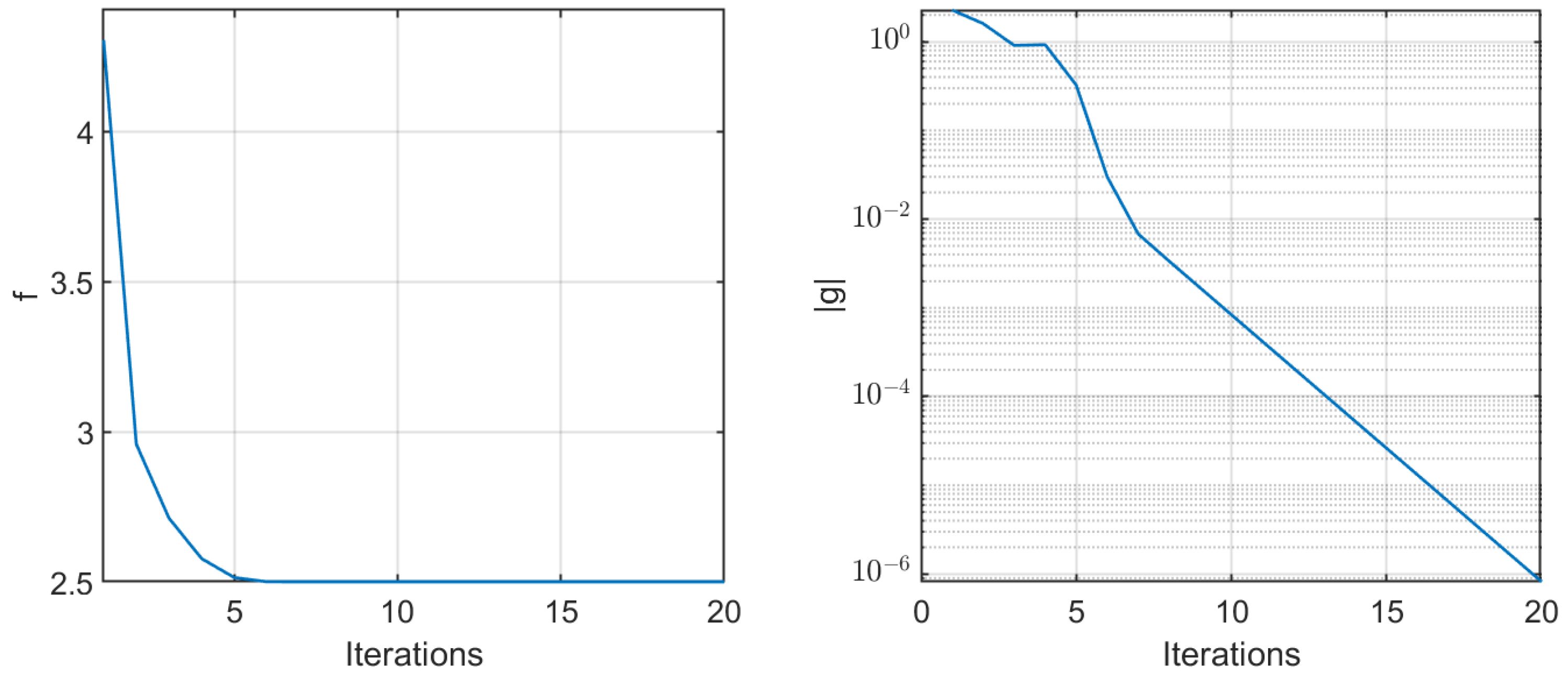
We first consider the biquadratic tensor in Example 2. The average iteration count for implementing Algorithm 1 is 18.55, the average CPU time consumed is $1.08\times {10}^{-1}$ seconds, and the average value of $\parallel \nabla f\left({\mathbf{z}}^{\infty }\right)\parallel$ is found to be $3.72\times {10}^{-7}$. Among all 20 repeated trials, an M-eigenvalue of 2.5 was achieved in 19 cases. We also show the values of M-eigenpairs in Table 4. Since for any M-eigenpair $(\lambda ,\mathbf{x},\mathbf{y})$, its variants $(\lambda ,-\mathbf{x},\mathbf{y})$, $(\lambda ,\mathbf{x},-\mathbf{y})$, $(\lambda ,-\mathbf{x},-\mathbf{y})$ are also M-eigenpairs of $\mathcal{A}$, we exclude these redundant M-eigenpairs from our results. Furthermore, we present the iterative procedure of Algorithm 1 for computing M-eigenvalues in Figure 1. It is evident that our Riemannian LBFGS algorithm exhibits rapid convergence.

Table 4. M-eigenpairs computed from Example 2.

$\mathit{\lambda }$	${\mathit{x}}_1$	${\mathit{x}}_2$	${\mathit{x}}_3$	${\mathit{y}}_1$	${\mathit{y}}_2$	${\mathit{y}}_3$
2.5000	0.6533	−0.2706	0.7071	−0.6533	0.2706	0.7071
2.5000	−0.6533	0.2706	0.7071	0.6533	−0.2706	0.7071
2.5000	0.2706	0.6533	0.7071	0.2706	0.6533	−0.7071
2.5000	0.2706	0.6533	−0.7071	0.2706	0.6533	0.7071
3.0000	0.6088	−0.7933	0.0003	−0.9915	−0.1304	0.0003

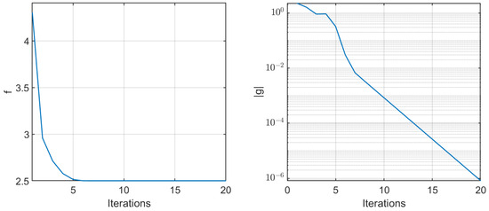
Figure 1. The iterative procedure of Algorithm 1 for computing M-eigenvalues of the biquadratic tensor $\mathcal{A}$ in Example 2. The left panel shows the objective function, while the right panel displays the norm of the gradient.

At last, we present an example from statistics.

Example 4.

We generate a sequence of 10,000 independent and identically distributed random matrices $X^{\left(t\right)}\in {\mathbb{R}}^{m\times n}$ uniformly from the interval $[0,10]$. Subsequently, we compute the covariance tensor by (3).

We show the numerical results for computing M-eigenvalues of the covariance biquadratic tensors by Algorithm 1 in Table 5. Here, ‘$\lambda$’ represents the smallest M-eigenvalue obtained from 20 repeated trials, and ’Rate’ denotes the success rate of returning the smallest M-eigenvalue. Additionally, ’Iteration’, ’Time (s)’, and ’Res’ correspond to the average values of the number of iterations, the CPU time consumed, and the norm of the gradient $\parallel \nabla f\left(\mathbf{z}\right)\parallel$ at the final iteration, respectively.

Table 5. Numerical results for computing M-eigenvalues of the covariance biquadratic tensors in Example 4 by Algorithm 1.

m	n	$\mathit{\lambda }$	Rate	Iteration	Time (s)	Res
5	5	7.8142	35%	30.75	0.331	2.15 $\times {10}^{-7}$
	10	7.7351	25%	44.80	0.295	2.22 $\times {10}^{-7}$
	20	7.4446	40%	54.90	0.442	2.99 $\times {10}^{-7}$
	30	7.3370	20%	57.35	0.527	5.26 $\times {10}^{-7}$
10	5	7.7211	45%	43.05	0.319	2.64 $\times {10}^{-7}$
	10	7.5963	20%	47.65	0.352	4.17 $\times {10}^{-7}$
	20	7.3332	15%	64.70	0.643	5.42 $\times {10}^{-7}$
	30	7.2051	5%	80.70	1.102	5.17 $\times {10}^{-7}$

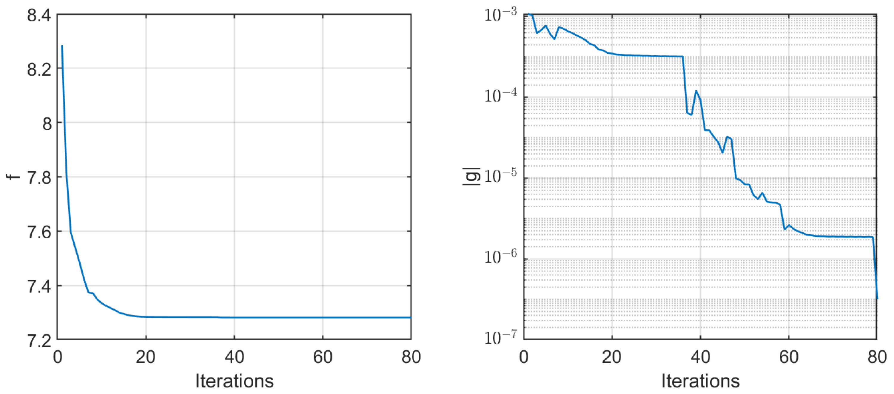
It is confirmed that all the smallest eigenvalues obtained are positive, which aligns with Proposition 2, indicating that the covariance tensor is positive definite. The success rate remains high for small-dimensional problems but gradually decreases as the values of m and n increase. This observation is consistent with the theoretical expectation that the number of M-eigenvalues for a higher-dimensional biquadratic tensor generally increases, leading to more KKT points and potentially greater difficulty in converging to the global optimal solution. Furthermore, the number of iterations is consistently below 100, and the gradient norm is smaller than the specified tolerance of ${10}^{-6}$ in all cases. At last, we present the iterative procedure of Algorithm 1 for computing M-eigenvalues of the covariance tensor with $m=10$ and $n=30$ in Figure 2. It is evident that our Riemannian LBFGS algorithm exhibits rapid convergence.

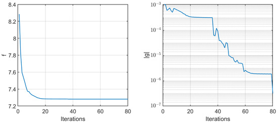
Figure 2. The iterative procedure of Algorithm 1 for computing M-eigenvalues of a nonsymmetric covariance tensor with $m=10$ and $n=30$ in Example 4. The left panel shows the objective function, while the right panel displays the norm of the gradient.

8. Final Remarks

Motivated by applications, in this paper, we extend the definition of M-eigenvalues of symmetric biquadratic tensors to nonsymmetric biquadratic tensors, show that M-eigenvalues always exist, a biquadrtic tensor is positive semi-definite (definite) if and only if its M-eigenvalues are nonnegative (positive). We present a Gershgorin-type theorem, several structured biquadratic tensors, and an algorithm for computing the smallest M-eigenvalue of a biquadratic tensor. We may explore further in the following three topics.

• Study more precise bounds for M-eigenvalues of biquadratic tensors and construct more efficient algorithms for computing the smallest M-eigenvalue of a biquadratic tensor.
• Identify more classes of structured biquadratic tensors.
• Study the SOS problem of biquadratic tensors.

References

- Qi, L.; Hu, S.; Zhang, X.; Xu, Y. Biquadratic tensors, biquadratic decomposition and norms of biquadratic tensors. Front. Math. China 2021, 16, 171–185. [Google Scholar] [CrossRef]
- Huang, Z.H.; Li, X.; Wang, Y. Bi-block positive semidefiniteness of bi-block symmetric tensors. Front. Math. China 2021, 16, 141–169. [Google Scholar] [CrossRef]
- Kolda, T.G.; Bader, B.W. Tensor decomposition and applications. SIAM Rev. 2009, 51, 455–500. [Google Scholar] [CrossRef]
- Knowles, J.K.; Sternberg, E. On the failure of ellipticity of the equations for finite elastostatic plane strain. Arch. Ration. Mech. Anal. 1976, 63, 321–336. [Google Scholar] [CrossRef]
- Zubov, L.M.; Rudev, A.N. On necessary and sufficient conditions of strong ellipticity of equilibrium equations for certain classes of anisotropic linearly elastic materials. J. Appl. Math. Mech. 2016, 9, 1096–1102. [Google Scholar] [CrossRef]
- Bomze, I.M.; Ling, C.; Qi, L.; Zhang, X. Standard bi-quadratic optimization problems and unconstrained polynomial reformulations. J. Glob. Optim. 2012, 52, 663–687. [Google Scholar] [CrossRef]
- Chen, Y.; Hu, Z.; Hu, J.; Shu, L. Block structure-based covariance tensor decomposition for group identification in matrix variables. Stat. Probab. Lett. 2025, 216, 110251. [Google Scholar] [CrossRef]
- Xiang, H.; Qi, L.; Wei, Y. M-eigenvalues of the Riemann curvature tensor. Commun. Math. Sci. 2018, 16, 2301–2315. [Google Scholar] [CrossRef]
- Yan, J.; Yin, X.; Lin, W.; Deng, C.; Zha, H.; Yang, X. A short survey of recent advances in graph matching. In Proceedings of the 2016 ACM on International Conference on Multimedia Retrieval, New York, NY, USA, 6–9 June 2016; pp. 167–174. [Google Scholar]
- Cui, C.; Qi, L.; Xu, Y. PSD and SOS biquadratic polynomials. Mathematics 2025, 13, 2294. [Google Scholar]
- Ling, C.; Nie, J.; Qi, L.; Ye, Y. Biquadratic optimization over unit spheres and semidefinite programming relaxations. SIAM J. Optim. 2010, 20, 1286–1310. [Google Scholar] [CrossRef]
- Qi, L.; Dai, H.H.; Han, D. Conditions for strong ellipticity and M-eigenvalues. Front. Math. China 2009, 4, 349–364. [Google Scholar] [CrossRef]
- Nye, J.F. Physical Properties of Crystals: Their Representation by Tensors and Matrices, 2nd ed.; Clarendon Press: Oxford, UK, 1985. [Google Scholar]
- Che, H.; Chen, H.; Zhou, G. New M-eigenvalue intervals and application to the strong ellipticity of fourth-order partially symmetric tensors. J. Ind. Manag. Optim. 2021, 17, 3685–3694. [Google Scholar] [CrossRef]
- Li, S.; Li, C.; Li, Y. M-eigenvalue inclusion intervals for a fourth-order partially symmetric tensor. J. Comput. Appl. Math. 2019, 356, 391–401. [Google Scholar] [CrossRef]
- Li, S.; Chen, Z.; Liu, Q.; Lu, L. Bounds of M-eigenvalues and strong ellipticity conditions for elasticity tensors. Linear Multilinear Algebra 2022, 70, 4544–4557. [Google Scholar] [CrossRef]
- Zou, W.; He, Q.; Huang, M.; Zheng, Q. Eshelby’s problem of non-elliptical inclusions. J. Mech. Phys. Solids 2010, 58, 346–372. [Google Scholar] [CrossRef]
- Wang, Y.; Qi, L.; Zhang, X. A practical method for computing the largest M-eigenvalue of a fourth-order partially symmetric tensor. Numer. Linear Algebra Appl. 2009, 16, 589–601. [Google Scholar] [CrossRef]
- Rindler, W. Relativity: Special, General and Cosmological, 2nd ed.; Oxford University Press: Oxford, UK, 2006. [Google Scholar]
- Cooper, J.; Dutle, A. Spectra of uniform hypergraphs. Linear Algebra Appl. 2012, 436, 3268–3292. [Google Scholar] [CrossRef]
- Qi, L.; Luo, Z. Tensor Analysis: Spectral Theory and Special Tensors; SIAM: Philadelphia, PA, USA, 2017. [Google Scholar]
- Yang, Y.; Yang, Q. On solving biquadratic optimization via semidefinite relaxation. Comput. Optim. Appl. 2012, 53, 845–867. [Google Scholar] [CrossRef]
- O’Rourke, S.M.; Setlur, P.; Rangaswamy, M.; Swindlehurst, A.L. Relaxed biquadratic optimization for joint filter-signal design in signal-dependent STAP. IEEE Trans. Signal Process. 2018, 66, 1300–1315. [Google Scholar] [CrossRef]
- Hilbert, D. Über die Darstellung definiter Formen als Summe von Formenquadraten. Math. Ann. 1888, 32, 342–350. [Google Scholar] [CrossRef]
- Wang, C.; Chen, H.; Wang, Y.; Yan, H. An alternating shifted inverse power method for the extremal eigenvalues of fourth-order partially symmetric tensors. Appl. Math. Lett. 2023, 141, 108601. [Google Scholar] [CrossRef]
- Zhao, J.; Liu, P.; Sang, C. Shifted inverse power method for computing the smallest M-eigenvalue of a fourth-order partially symmetric tensor. J. Optim. Theory Appl. 2024, 200, 1131–1159. [Google Scholar] [CrossRef]
- Ding, W.; Liu, J.; Qi, L.; Yan, H. Elasticity M-tensors and the strong ellipticity condition. Appl. Math. Comput. 2020, 373, 124982. [Google Scholar] [CrossRef]
- Wang, G.; Sun, L.; Liu, L. M-eigenvalues-based sufficient conditions for the positive definiteness of fourth-order partially symmetric tensors. Complexity 2020, 2020, 2474278. [Google Scholar] [CrossRef]
- Qi, L. Eigenvalues of a real supersymmetric tensor. J. Symb. Comput. 2005, 40, 1302–1324. [Google Scholar] [CrossRef]
- Zhao, J. Conditions of strong ellipticity and calculation of M-eigenvalues for a partially symmetric tensor. Appl. Math. Comput. 2023, 458, 128245. [Google Scholar] [CrossRef]
- Qi, L.; Song, Y. An even order symmetric B tensor is positive definite. Linear Algebra Its Appl. 2014, 457, 303–312. [Google Scholar] [CrossRef]
- Jiang, B.; Yang, F.; Zhang, S. Tensor and its tucker core: The invariance relationships. Numer. Linear Algebra Appl. 2017, 24, e2086. [Google Scholar] [CrossRef]
- Nocedal, J.; Wright, S.J. Numerical Optimization, 2nd ed.; Springer Series in Operations Research and Financial Engineering; Springer: New York, NY, USA, 2006. [Google Scholar]
- Chang, J.; Chen, Y.; Qi, L. Computing eigenvalues of large scale sparse tensors arising from a hypergraph. SIAM J. Sci. Comput. 2016, 38, A3618–A3643. [Google Scholar] [CrossRef]
- Bolte, J.; Sabach, S.; Teboulle, M. Proximal alternating linearized minimizationfor nonconvex and nonsmooth problems. Math. Program. Ser. A 2014, 146, 459–494. [Google Scholar] [CrossRef]
- He, J.; Li, C.; Wei, Y. M-eigenvalue intervals and checkable sufficient conditions for the strong ellipticity. Appl. Math. Lett. 2020, 102, 106137. [Google Scholar] [CrossRef]
Disclaimer/Publisher’s Note: The statements, opinions and data contained in all publications are solely those of the individual author(s) and contributor(s) and not of MDPI and/or the editor(s). MDPI and/or the editor(s) disclaim responsibility for any injury to people or property resulting from any ideas, methods, instructions or products referred to in the content. |
© 2025 by the authors. Licensee MDPI, Basel, Switzerland. This article is an open access article distributed under the terms and conditions of the Creative Commons Attribution (CC BY) license (https://creativecommons.org/licenses/by/4.0/).