Abstract
We investigate serval models for two scalar fields in one space dimension with topologically stable solitons that are constructed from BPS equations. The asymptotic behavior of these solitons fully determines their classical energies. A particular feature of the considered models is that there are several translationally invariant ground states that we call primary and secondary vacua. The former are those that are asymptotically assumed by the solitons. Solitons that occupy a secondary vacuum in finite but eventually large portions of space are classically degenerate. Thus the quantum contributions to the energies are decisive for the energetically favored soliton. While some of these solitons were constructed previously, we, for the first time, compute the leading (one-loop) quantum contribution their energies. In all cases considered we find that this contribution is not bounded from below and that it is the more negative the larger the region is in which the soliton approaches a secondary vacuum. This corroborates the conjecture, earlier inferred from the Shifman-Voloshin soliton, that the availability of secondary vacua destabilizes these solitons on the quantum level.
1. Introduction
Even though strictly speaking they are solitary waves, we use the notion solitons [1,2,3,4] for solutions to non-linear field equations that have localized (classical) energy densities and finite total energies. Examples for solitons in physics are Skyrmions [5,6], monopoles in space-time dimensions [7,8] and vortices, strings and lumps in [9,10,11]. Solitons have almost uncountable applications in various disciplines: in cosmology [12], condensed matter physics [13,14], magnetic systems [15] as well as hadron [16] and nuclear physics [17]. We point to those textbooks and review articles for more details and further references.
Here we focus on particular models with two scalar fields, and , in which have the particular feature of possessing two translationally invariant minimal energy configurations that we call primary and secondary vacua. In addition these models have Bogomol’nyi-Prasad-Sommerfield (BPS) [18,19] constructions that simplify the static soliton equations to first order differential equations. Within BPS constructions the classical energies are fully determined by the solitons’ asymptotic values [20]. While the solitons assume primary vacua at spatial infinity and are kink-like ( can be smoothly modified into the hyperbolic tangent function without changes at spatial infinity), they may dwell in a secondary vacuum within a finite region of space. We will see that the solitons are classically degenerate in a single, continuous parameter that controls size of that region. Because of that degeneracy there is no unique classical soliton and the quantum contribution to the energy, even if small when compared to the classical energy, will decide which is the energetically favored soliton. This scenario has recently been investigated for the Shifman-Voloshin-soliton [21]. It was found that, as a function of that single parameter, the leading, one-loop quantum correction to the energy, the so-called vacuum polarization energy (VPE) did not have a lower bound [22]. Hence no stable soliton exists in that model at the one-loop quantum level. It was hence conjectured that such quantum destabilization scenarios will occur whenever the soliton has access to a secondary vacuum. Here we will provide further examples to corroborate that conjecture.
We will employ spectral methods [23] to compute the VPE. These methods have been demonstrated to be very efficient when expressing the contribution from the continuum quantum fluctuations as an integral over imaginary momenta [24]. In Section 3 we will explain that the spectral methods yield the VPE from solving a single differential equation for the quantum fluctuations in the soliton background. This will also reveal that these methods can be applied straightforwardly and are less intricate than other methods as, for example, the heat kernel expansion [25] which has also been applied [26] to particular soliton solutions of the Shifman-Voloshin model. We will adopt the simple no-tadpole renormalization scheme that fully removes the ultraviolet divergent Feynman diagrams. In this scheme is equivalent to the formalism of Ref. [27] which has recently been linked to a normal-ordering description [28]. For the prime example of the kink in the model, the no-tadpole prescription yields [23] the historic Dashen-Hasslacher-Neveu result [29].
In Section 2 we will discuss the properties of the BPS construction for the models under consideration. The relevant techniques from the spectral methods will be provided in Section 3. Section 4 contains our results, both for the construction of the solitons as well as their VPEs. Some concluding comments are contained in Section 5.
This article contains quite a number of mathematical symbols. We summarize and describe them in Table 1.

Table 1.
Mathematical symbols used in the text and their meaning.
2. General Structure of the Sample Models
The models that we will discuss are defined by so-called super-potentials [30] whose derivatives specify the Lagrangian
Here dots and primes denote time (t) and space (x) derivatives, respectively. For static configurations, the classical energy then becomes a BPS construction
where the signs must be chosen such that the boundary contribution is non-negative. Once the boundary values of the fields at positive and negative spatial infinity are prescribed, is minimized by the solutions to the first order equations
As a consequence whatever the solutions to the above equations look like.
Typically the super-potential is an even function of but it is odd in . Then vanishes whenever does. In turn and will, respectively, be odd and even functions of the spatial coordinate when the coordinate system is defined such that . Hence the only undetermined initial condition for the BPS Equations (3) is . Without loss of generality we may take and so that the upper sign applies in Equations (2) and (3). Requiring that is a monotonous function (like the -kink) then constrains . Depending on the model parameters this condition can be fulfilled for a range of values . If so, the classical energy will be degenerate in and the quantum correction to the energy will decide on the favored configuration.
Furthermore we have to specify the notion of primary and secondary vacua that correspond to the translationally invariant solutions of the BPS Equations (3). With the above mentioned properties of the super-potential under sign changes of the fields, when so that has (at least) two solutions (The two solutions must have opposite signs which allowed us to set above.) for . These are primary vacua and the soliton assumes one of them at negative spatial infinity and another one at the other end of the universe. As already mentioned, when . We can thus construct an alternative solution to by determining a constant, non-zero from . This is also a zero energy configuration which we call the secondary vacuum because we cannot build a (topological) soliton on top of it. The reason being that the profiles at positive and negative spatial infinity would be equal since is invariant under spatial reflection. However, by varying we can find solitons on top of primary vacua that approach such a secondary vacuum configuration within a finite but eventually large portion of space. It is exactly this scenario that we will investigate for a number of models. We will also encounter situations in which the secondary vacuum has both and .
3. Vacuum Polarization Energy (VPE)
Here we briefly describe the computation of the VPE, i.e., the leading quantum contribution to the total energy, in the framework of spectral methods for the case of two scalar fields in . These methods are by now well-established and in particular their almost effortless use when continuing the momenta of the scattering modes to the complex plane has recently been reviewed [24].
The point of departure is to parameterize the two fields as
The index stands for either the or fields. The superscript refers to the soliton solutions constructed above and we have omitted the frequency argument for the small amplitude fluctuations . They are subject to the second order differential equations
that emerge from substituting the parameterization, Equation (4) into the Euler-Lagrangian equations derived from the Lagrangian , Equation (1) and linearizing in . While contains the mass parameters, the potential matrix,
is generated by the soliton profiles and thus is time-independent so that different frequency modes decouple. The mass parameters are determined from the model parameters such that plane waves solve Equation (5) for , which follows for a primary vacuum configuration. Once and are determined, we map the fields and onto and such that . We will provide more details on the matrices M and V in the context of the particular models in Section 4.
The VPE is computed as the renormalized sum of the shift in the zero-point energies
The are the energy eigenvalues in Equation (5) and are their counterparts for . The counterterm contribution, emerges from substituting the soliton profiles into the counterterm Lagrangian that cancels the ultra-violet divergences in the sum over the eigenmodes. In we only need a single counterterm and we implement the no-tadpole condition to fix its finite piece. This condition removes the contribution from the sum. We can indeed remove this contribution fully and not only at a particular renormalization scale because the only ultra-violet divergent Feynman diagram has a loop that starts and ends at the same point and thus does not depend on the momenta of the external line(s). We will compute the sum in Equation (7) from scattering data extracted from the solutions to Equation (5). The Born approximation to these data is . Hence with the no-tadpole condition we merely subtract the Born approximation from the scattering data expression for the sum in Equation (7) and then drop completely.
The sum, Equation (7) has contributions from discrete bound states and continuous scattering states . For the considered scenarios there are typically two zero mode bound states. One for the translational symmetry and one that arises because the classical energy is invariant when is varied. There may be further bound states depending on the peculiarities of the models. The continuum contribution is computed by integrating the dispersion relation weighted by the change of the density of states induced by the soliton, [29,31] where the phase shift is extracted from the scattering matrix: . However, for numerical purpose, the phase shift is not computed from the scattering matrix but rather we use that the phase shift is the phase of the Jost function which by itself is extracted from solutions to Equation (5) that resemble out-going plane waves as . This function is analytic in the upper half of the complex momentum plane and has zeros at the imaginary wave-numbers of the bound states [32]. With the subtraction of its Born approximation we can then compute the integral over the continuum modes as a contour integral because there is no contribution from the semi-circle at . Furthermore the above mentioned zeros produce poles in the logarithmic derivative of the phase of the Jost function and cancel the explicit bound state contribution in Equation (7). All what is left in the contour integral is the contribution from circling the branch cut in along the imaginary axis for and . After a final integration by parts we are left with a very compact formula for the VPE
where is logarithm of the Jost function and is its Born approximation. In either case a sum of scattering channels is understood.
Next we recall the calculation of the Jost function for theories with two fields in which has been developed in Ref. [33] for the case that there is some kind of symmetry that relates the wave-equation for and . Starting point is the Jost solution that we elevate to a matrix function
and . The elements within a given column represent the two fields while the two columns represent the scattering channels, i.e., out-going plane waves for only either the or fields. The prescription for the momentum of the heavier field ensures that is also analytic in the gap . Yet, this problem does not occur when, as motivated above, the VPE is computed from imaginary momenta (See Ref. [34] for the real momenta version.). The scattering wave-function, , is a linear combination of and . Assuming, for the time being, that the symmetric (S) and anti-symmetric (A) channels decouple, the corresponding scattering matrices are obtained from and . That is, the scattering matrices are determined from and . The phase shifts are then expressed in terms of and . We will not present these expression but rather turn to the imaginary axis formulation and write for the analytically continuated factor matrix, whose second order differential equation is
and . The analytically continued combinations of and that enter are
These are the so-called Jost matrices in the symmetric and anti-symmetric channels. For the problem at hand the symmetric and anti-symmetric channel do, unfortunately, not decouple. The field potential in Equation (1) is even in both fields. Hence the diagonal elements of the scattering potential, Equation (6) are even functions of both fields while its off-diagonals are odd. With the above discussed properties of the profiles, it is then obvious that . Therefore the scattering problem decouples in the parity channels and the relevant Jost matrices are [33]
with projectors as well as modified factor matrices and . The combinations in Equation (12) essentially exchange the second (first) rows of and for the positive (negative) parity channel and add appropriate kinematic factors. From this we find the relevant logarithm that enters Equation (8)
since the sum of the logarithms is the logarithm of the product. The off-diagonal elements of only enter at second order. Hence the Born approximation is just the sum of the Born approximations for the decoupled problem,
Now we have collected all entries to compute the VPE in the no-tadpole renormalization scheme.
As we have summarized the theoretical background, we briefly describe the numerical treatment leading to the VPE as a function of . Generally, all differential equations are integrated with Runge-Kutta algorithms combined with adaptive step size controls. For a particular model described by the superpotential W we determine the vacua, in particular the secondary vacuum of the second scalar field, as functions of the model parameters. Then we prescribe (and ) to solve the first order Equations (3). This yields arrays of the profile functions and at distinct points . (In all numerical computations ‘∞’ refers to a numerical value large enough so that the numerical results are stable under moderate changes of this value.) These arrays enter the scattering potential . Typically the adaptive step size control requires the potential at points and we interpolate between neighboring points. Using we then integrate the differential Equation (10) to obtain and . To determine the (imaginary) momentum t for which we actually integrate the differential Equation (10) we define the function subject to the differential equation
so that . Integrating this differential equation with an adaptive step control is advantageous because it carefully treats the logarithmic behavior of for that originates from the zero modes. This behavior also requires a very tiny lower bound, when numerically integrating the above differential equation. Within a given model we finally obtain as a function of the variational parameter a defined by .
4. Sample Models
We introduce dimensionless variables and fields. This rescaling leaves an overall factor for the Lagrangian which does not affect the classical equations of motion. However, it enters the relation between the canonical field momenta and their velocities. In turn it acts as a loop-counter in the sense that it is a relative weight between and . Fortunately, for a given model with fixed model parameters, we will only compare the VPEs for configurations with equal so that this relative factor is not relevant.
In all numerical calculations we adopt sign conventions such that the kink-like profile, connects a positive primary vacuum at negative spatial infinity to its negative counterpart at positive spatial infinity. Furthermore we take all model parameters to be non-negative.
As a reminder we list the super-potential of the Shifman-Voloshin model [21], see also [35],
The primary vacua are at and . The secondary vacua are at and . Solutions (that are classically degenerate) exist for and, as shown in Ref. [22], the VPE does not have a lower bound as except for the particular case of for which the model can be mapped onto a model with two decoupled scalar fields that have the standard quartic interaction with spontaneous symmetry breaking. We next turn to three further models that exhibit similar features.
In the following we will discuss solitons in three other models with secondary vacua. We will encounter that the structure of these secondary vacua varies with the model parameters. We will tabulate numerical results for our main objective, the VPEs in these models, as functions of the model parameters and, more enlightening, as functions of the variational parameters that distinguish the classically degenerate solitons. The dependencies of the VPEs on these variational parameters will be our central results.
4.1. Model A
We replace the last term in Equation (15) by a sine-Gordon type interaction and introduce a second model parameter
From the super-potential in Equation (16) we get the static BPS equations
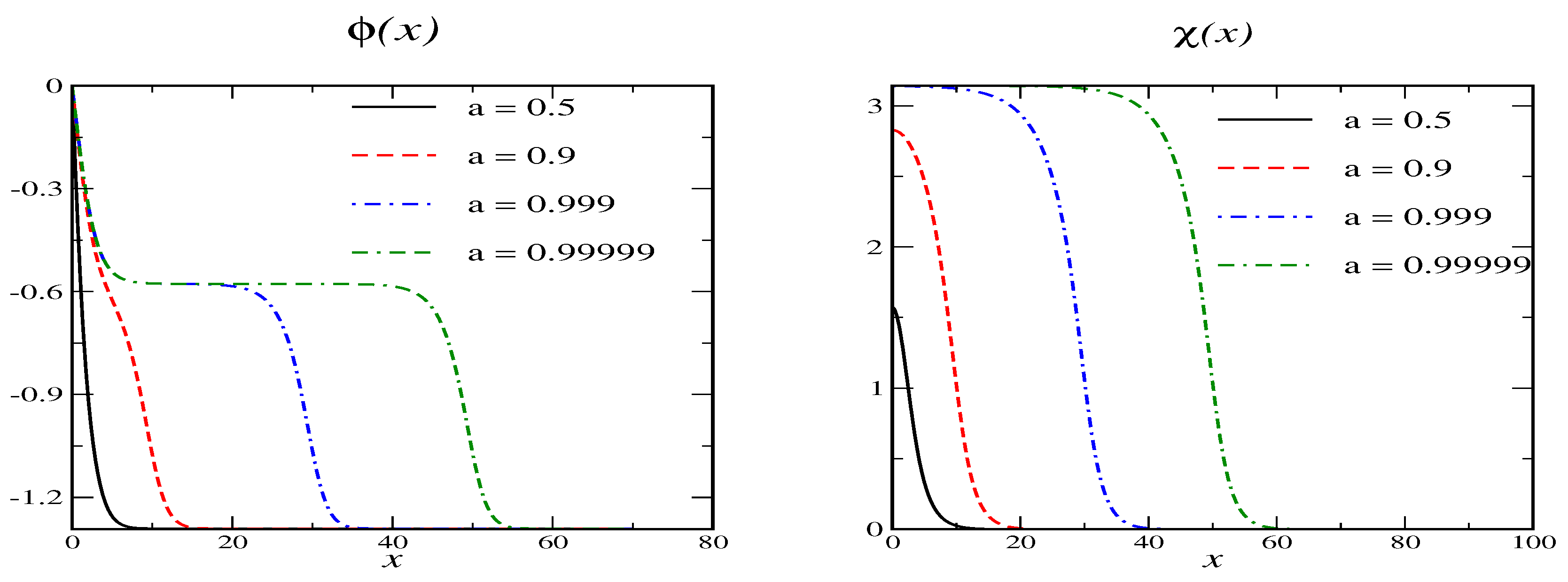
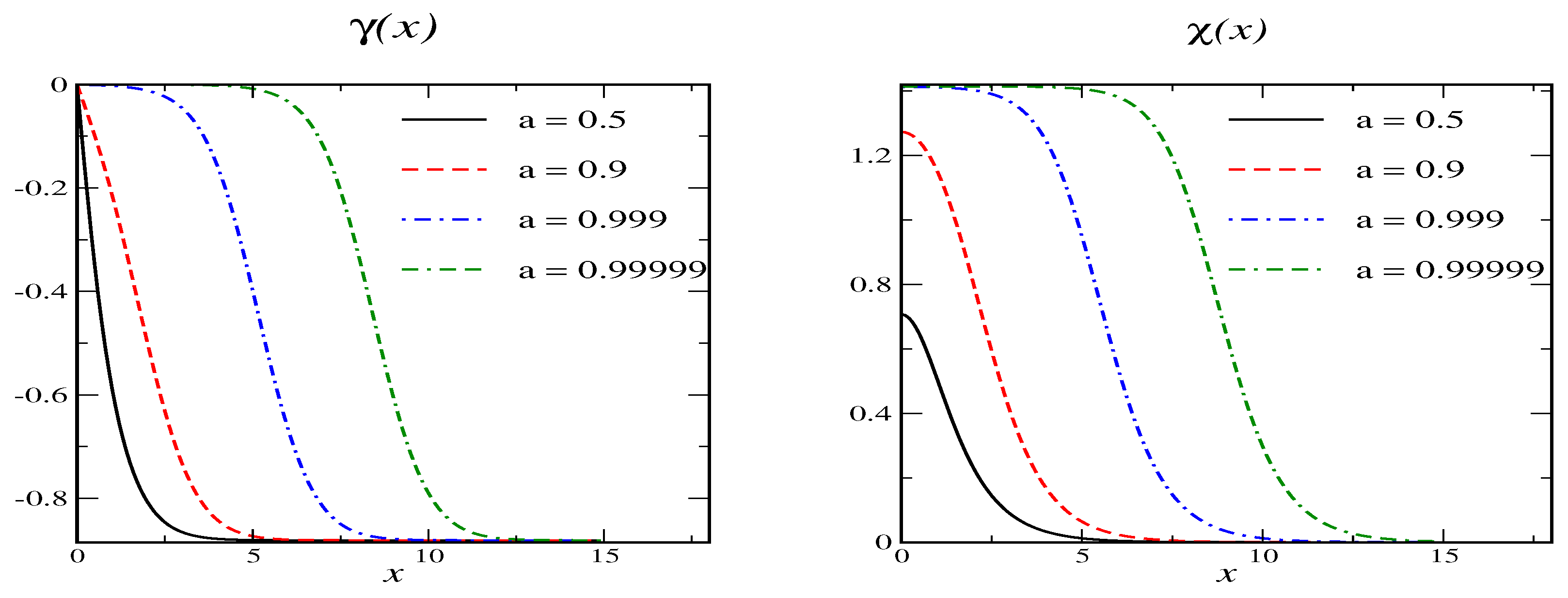
The primary vacua are at and . We expand the fields around these vacua and read of the mass parameters and . For the secondary vacua are obviously at and and the situation is similar to the Shifman-Voloshin model. Examples for the soliton profiles are shown in Figure 1 for various values of . While, by construction, the profiles approach a primary vacuum at spatial infinity, they occupy a secondary vacuum in an ever increasing region as . Of course, the classical energy, does not depend on a.
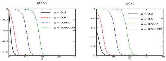
Figure 1.
Soliton profiles for model A with and for various values of the variational parameter a. The secondary vacuum has and .
The computation of the VPE requires the potential matrix (for the case so that and )
with and . By substituting the soliton profiles for and we compute the VPE with the formalism of Section 3. Not surprisingly we find that it does depend on the degeneracy parameter a. Neither are we surprised that the VPE does not have a lower bound as can be inferred from Table 2 in which we list the VPE for numerous values of .
Table 2.
VPE for model A as a function of the model parameter and the variational parameter a for .
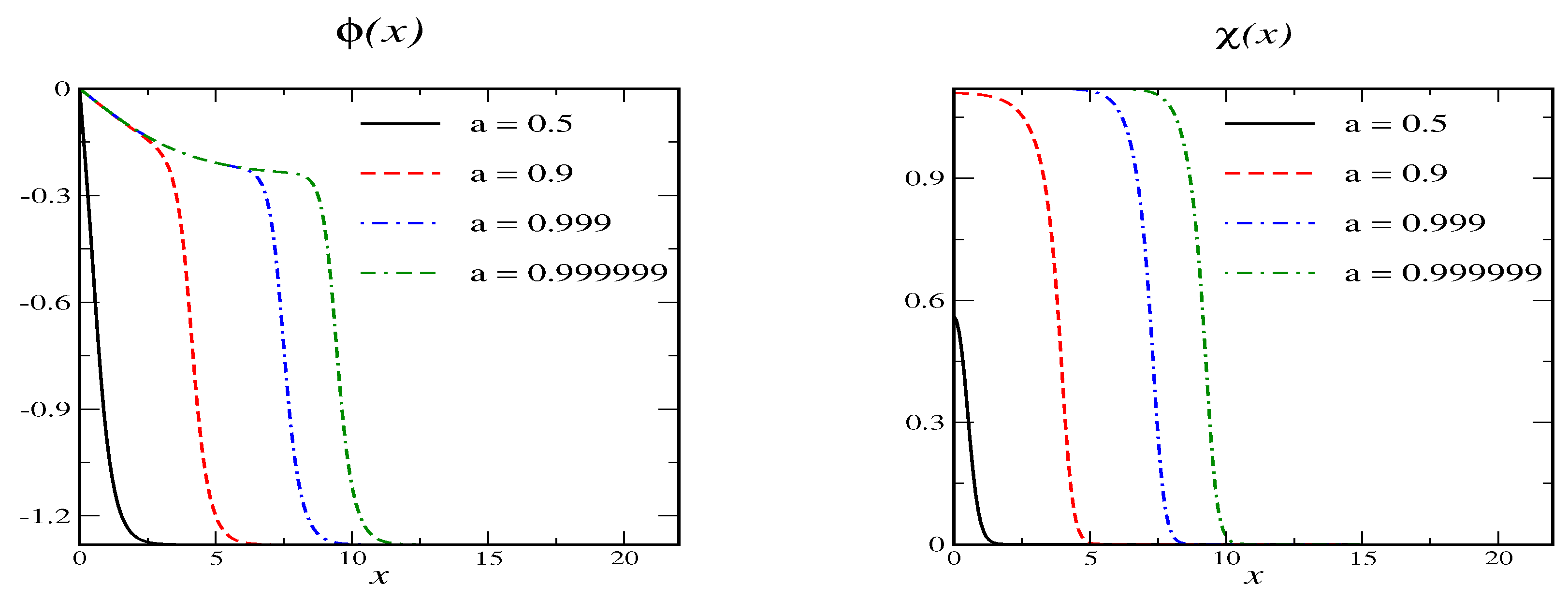
For and we cannot accommodate . However, there is a secondary vacuum since when and then we have for . Such a scenario is not contained in the Shifman-Voloshin model. Examples for the resulting soliton profiles are shown in Figure 2 for various values of the variational parameter .
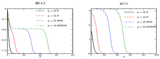
Figure 2.
Soliton profiles for model A with and for various values of the variational parameter a. Here the secondary vacuum is at and .
As a tends to one, the profile remains in that secondary vacuum for an ever growing region while the profile quickly drops from zero to its secondary vacuum value. Again, the VPE does not have a lower bound as the region grows in which the profiles assume their secondary vacua. In Table 3 we list the for an exemplary set of model parameters as a function of a for the scenario that has .
Table 3.
Same as Table 2 for various model parameters and .
In Figure 3 we verify that as for both and the VPE essentially approaches negative infinity like . Obviously there is no lower bound to the VPE and the quantum effects tend to destabilize this soliton whatever the secondary vacuum is.
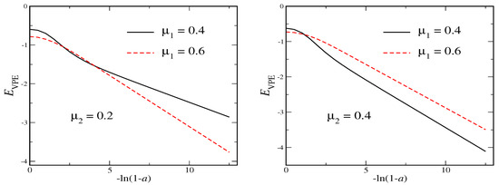
Figure 3.
The VPE for the model defined in Equation (16) as a function of the variable that measures the deviation from the secondary vacuum.
4.2. Model B
The next model is characterized by the super-potential
leading to the BPS equations
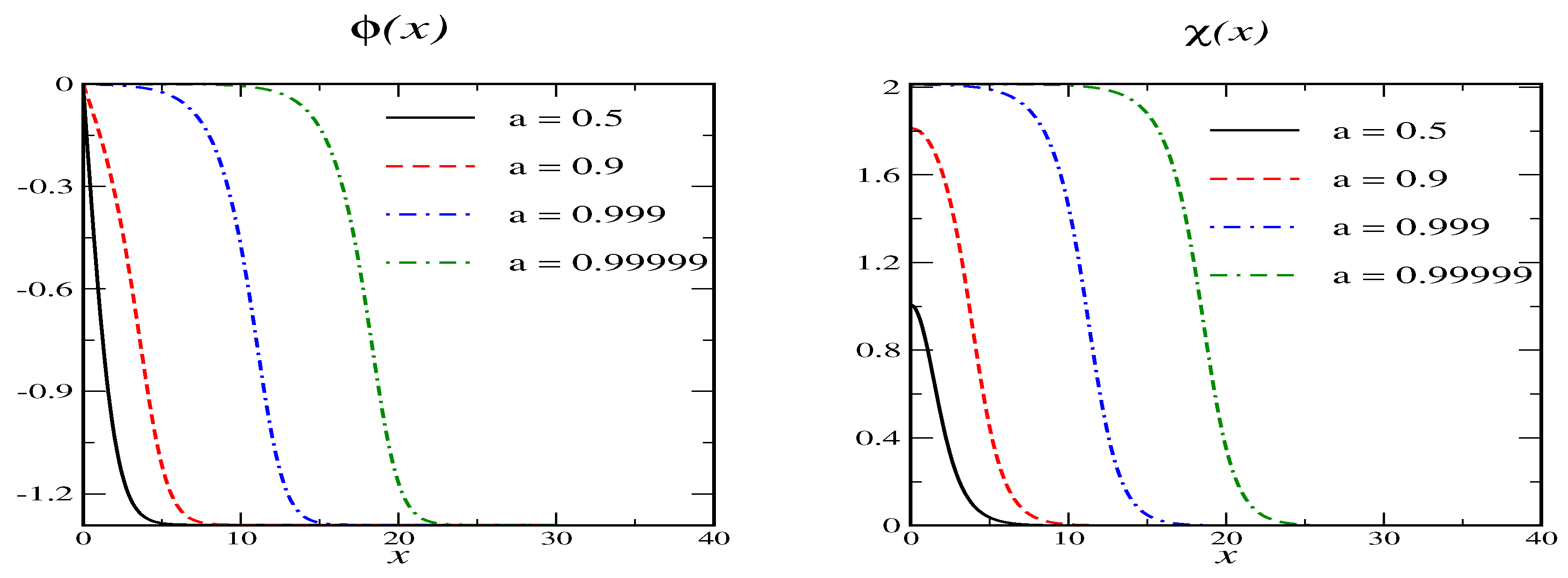
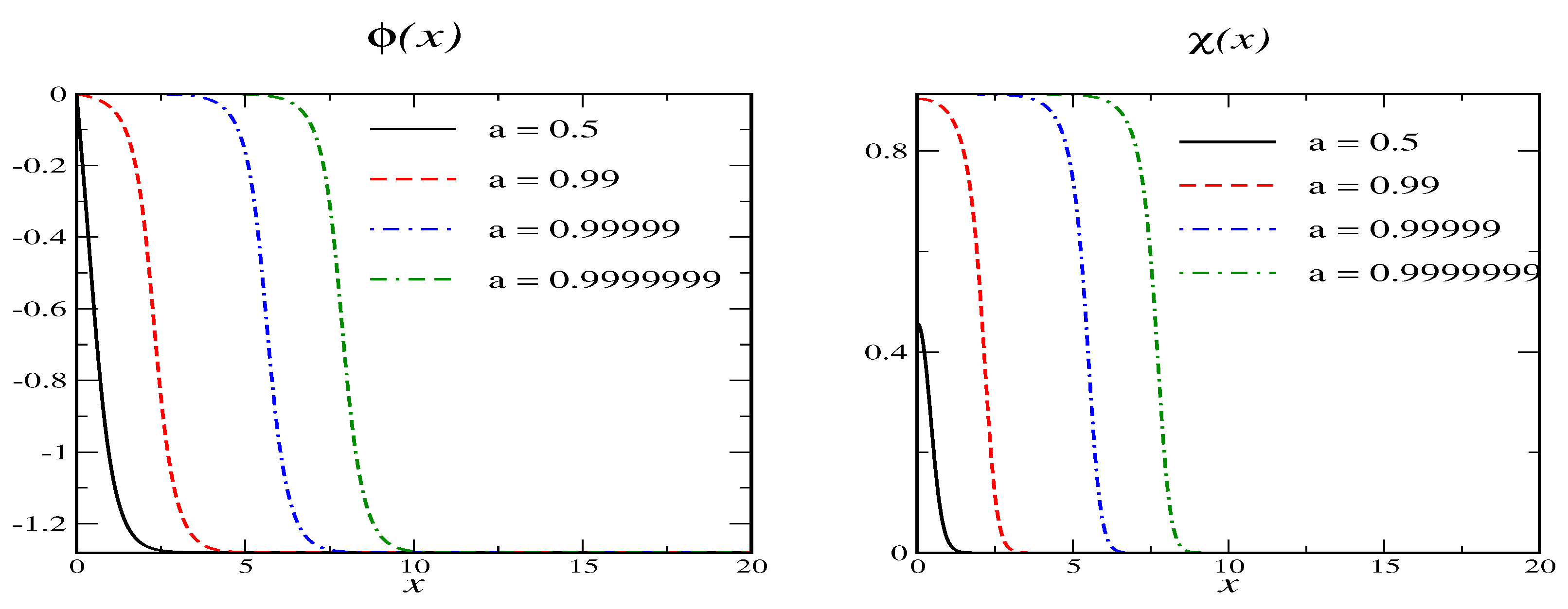
The primary vacua are at and . The associated mass parameters are and . When , or equivalently there are secondary vacua at and . If we want to construct soliton solutions whose profiles decrease monotonously so that with and , the right-hand-sides in Equation (20) may not be positive. This requires . Parameterizing the right hand side of the differential equation for is non-positive for and only when the above condition on the secondary vacuum is fulfilled. That is, the conditions on the secondary vacuum and the existence of a soliton are identical. A sample soliton solution is shown in Figure 4. The behavior generalizes: as the profiles approach a secondary vacuum in a large portion of space. However, that portion does not include because in that vacuum.
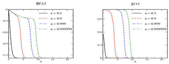
Figure 4.
Soliton profiles for model B with and for various values of the variational parameter a. The secondary vacuum has and .
We abstain from presenting the potential matrix V for this model and directly move to the discussion of our numerical results for the VPE. To explore the parameter dependence efficiently we write with . The results in terms of the model parameter b and the variational parameter a are listed in Table 4.
Table 4.
Vacuum polarization energy for the model defined by the super-potential Equation (19) for . The parameters b and a, respectively, determine the model parameter and initial value of the profile , cf. text.
Again we can fit a function linear in to the VPE for . We find that the critical value for a at which this behavior sets in increases with b. In any event, there is no lower bound for the VPE suggesting again that the soliton is not stable. The effect is the more pronounced as the model parameters get closer to the limiting case for which the soliton accesses the secondary vacuum.
As , approaches zero in the secondary vacuum. When exceeds unity, stays at zero but decreases from to in the secondary vacuum. (The configuration with the positive square root is also a solution but does not support stable solitons.) A set of soliton solutions for the parameterization and is shown in Figure 5.
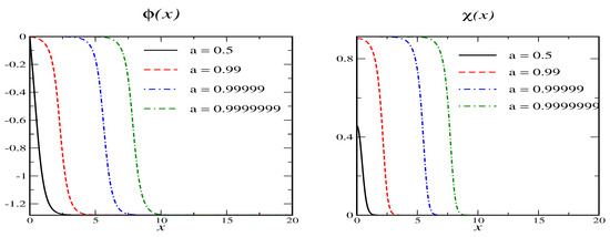
Figure 5.
Soliton profiles for model B with and for various values of the variational parameter a. The secondary vacuum has and .
The notation for the model parameters remains unchanged, but now we take . As before, for large enough a we can approximate the VPEs listed in Table 5 by a function that is linear in .
Table 5.
Vacuum polarization energy for the model defined by the super-potential Equation (19) for . The parameters b and a, respectively, determine the model parameter and initial value of the profile , cf. text.
4.3. Model C
This model is taken from Ref. [36]. It is motivated by the super-potential of model A but subsequently the kink-type field is written as , so that the metric in the field space depends on the fields. To return to a constant metric but nevertheless have a BPS construction the super-potential is modified to
The fact that this potential is only known as an indefinite integral is not really a problem. We would need to integrate from to for the classical energy. The integral is over rather than the spatial coordinate and thus is not sensitive to the form of the soliton.
For the BPS equations we only require the -derivative of that integral yielding
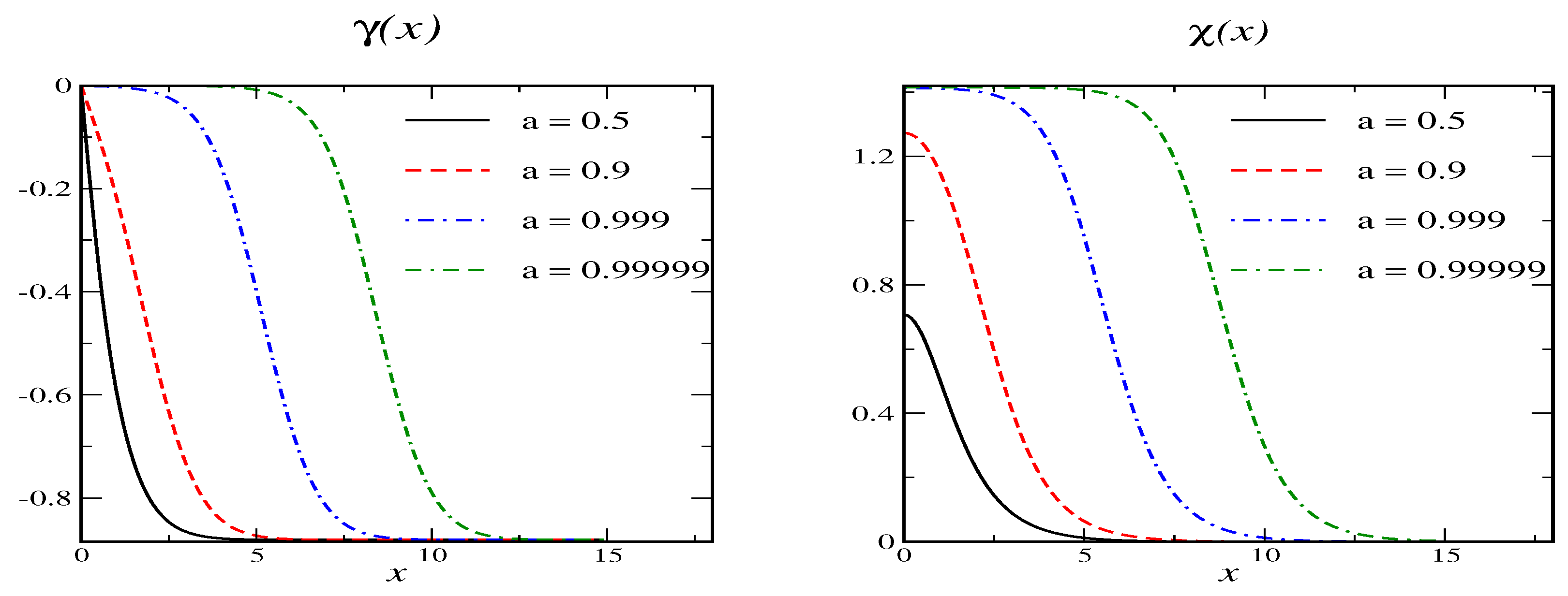
Again the primary vacua are at and while the secondary vacua are at and . We therefore introduce the variational parameter a in the initial condition . As long as , the right-hand-side of is negative for and any value of . Hence we expect degenerate solutions for all . The inequality arises from the demanding that the right-hand-side of is negative when and . Furthermore the mass parameters and are obtained from expanding Equation (22) around the primary vacuum (). Thus the existence of a BPS soliton on top of the above mentioned primary vacua yields the upper bound . Profiles determined subject to this condition are shown in Figure 6.
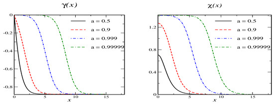
Figure 6.
Soliton profiles and for model C with . The secondary vacuum has and .
We observe the by now familiar behavior that the soliton approaches the secondary vacuum as .
Again we abstain from displaying the bulky expressions for the scattering potential and immediately list the numerical results for the VPE in Table 6.
Table 6.
VPE of model C for different values of the model parameter and the variational parameter a.
For and the right-hand-side of the differential equation for has another zero at or , which is less than 1 for . In that case the soliton assumes at spatial infinity (This configuration actually is a maximum of the action density for .). The mass parameters for these primary vacua are and . The expressions for the secondary vacua are as in the case with .
From the graphs in Figure 7 and the data in Table 7 we observe that the resulting VPEs show the same tendency as the other models (including the Shifman-Voloshin case) to approach negative infinity like .
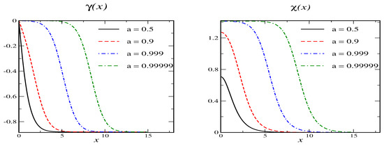
Figure 7.
Soliton profiles and for model C with . The primary vacua are at or and . The secondary vacuum has and .
Table 7.
Same as Table 6 for .
4.4. A Note on Zero Modes
In the context of our numerical analysis we have verified the existence of the two zero modes mentioned in Section 3. With the current techniques an effortless way to do so is to numerically determine in for since the Jost function has zeros at the imaginary momenta associated with the bound state energies. In almost all cases the numerical fit indeed produced results consistent with . The only exceptions were observed in cases with the soliton being in secondary vacua with for large regions of space. In those cases the fit yielded . We then employed techniques as in section III of Ref. [33] and found that the third (would-be) zero mode was dynamical: it emerged from an ordinary bound state with a non-zero energy eigenvalue in the limit . When the secondary vacuum does not include , the profile has distinct plateaus along the negative and positive half-lines. Moving around those plateaus produces two independent zero modes in addition to the translational one.
5. Conclusions
We have investigated a number of BPS solitons in one space dimension. The models under consideration have several distinct translationally invariant zero energy solutions, at least for certain ranges of model parameters. We refer to these solutions as primary and secondary vacua. At negative spatial infinity topologically stable solitons approach a primary vacuum but its negative at the opposite end. Yet, the soliton may close in on a secondary vacuum in an arbitrarily large portion of space without any classical energy cost so that there are infinitely many classically degenerate solutions. We must then include the quantum corrections to identify the energetically favored solution. For this purpose we have computed the leading, one-loop quantum correction which is the vacuum polarization energy (VPE) of such solitons.
The sample models considered here have two scalar fields and with the corresponding static soliton profiles being respectively odd and even under spatial reflection. This guarantees topological stability and selects the primary vacua as those with . On the other hand the secondary vacua have . The value of in secondary vacua as well as other peculiarities of the secondary vacua depend on the model parameters. Further conditions on the availablility of these vacua arise from requiring the existence of localized static solutions.
We have introduced the variational parameter as the measure of how the spatially symmetric component of the soliton approaches its secondary vacuum, and have found that the classical energy is independent of a by the BPS construction. On the other hand the VPE decreases like with as and hence has no lower bound. In the same limit the soliton dwells in a secondary vacuum for an increasing and unbound region. Though and are model dependent, this functional behavior has been reproduced in all of the considered models. Hence our computations corroborate the earlier conjecture [22] that quantum corrections destabilize classically degenerate BPS solitons when they may approach secondary vacua in an arbitrarily large portion of space.
Eventually soliton solutions with constant and exist when . They connect and along the coordinate axis. These borderline cases have different classical energies when is not a primary vacuum. Since these solutions are merely variants of the ordinary kink we have not considered them here.
Of course, when the first order correction is sizable, higher orders may be as relevant. Studies on higher order quantum corrections for solitons have just recently commenced [37].
Author Contributions
Conceptualization, H.W.; Software, W.J.M.; Formal analysis, W.J.M. and H.W.; Writing—original draft, H.W.; Writing—review and editing, W.J.M. and H.W.; All authors have read and agreed to the published version of the manuscript.
Funding
H.W. is supported in part by the National Research Foundation of South Africa (NRF) under grant 150672.
Data Availability Statement
The data supporting this study’s findings are available within the article.
Conflicts of Interest
The authors declare no conflicts of interest.
References
- Rajaraman, R. Solitons and Instantons; North Holland: Amsterdam, The Netherlands, 1982. [Google Scholar]
- Manton, N.S.; Sutcliffe, P. Topological Solitons; Cambridge Monographs on Mathematical Physics; Cambridge University Press: Cambridge, UK, 2004. [Google Scholar]
- Vachaspati, T. Kinks and Domain Walls: An Introduction to Classical and Quantum Solitons; Oxford University Press: Oxford, UK, 2010. [Google Scholar]
- Weinberg, E. Classical Solitons in Quantum Field Theory; Cambridge University Press: Cambridge, UK, 2012. [Google Scholar]
- Skyrme, T.H.R. A nonlinear field theory. Proc. R. Soc. Lond. 1961, A260, 127–138. [Google Scholar]
- Zahed, I.; Brown, G.E. The Skyrme model. Phys. Rept. 1986, 142, 1–102. [Google Scholar] [CrossRef]
- ’t Hooft, G. Magnetic monopoles in unified gauge theories. Nucl. Phys. B 1974, 79, 276–284. [Google Scholar] [CrossRef]
- Polyakov, A.M. Particle spectrum in the quantum field theory. JETP Lett. 1974, 20, 194–195. [Google Scholar]
- Vachaspati, T. Vortex solutions in the Weinberg-Salam model. Phys. Rev. Lett. 1992, 68, 1977–1980, Erratum in Phys. Rev. Lett. 1992, 69, 216. [Google Scholar] [CrossRef]
- Achucarro, A.; Vachaspati, T. Semilocal and electroweak strings. Phys. Rept. 2000, 327, 347–426. [Google Scholar] [CrossRef]
- Nambu, Y. String-like configurations in the Weinberg-Salam theory. Nucl. Phys. B 1977, 130, 505–515. [Google Scholar] [CrossRef]
- Vilenkin, A.; Shellard, E.P.S. Cosmic Strings and Other Topological Defects; Cambridge University Press: Cambridge, UK, 2000. [Google Scholar]
- Schollwöck, U.; Richter, J.; Farnell, D.J.; Bishop, R.F. Quantum Magnetism; Lecture Notes Physics; Springer: Berlin/Heidelberg, Germany, 2004; Volume 645. [Google Scholar]
- Nagaosa, N.; Tokura, Y. Topological properties and dynamics of magnetic Skyrmions. Nat. Nanotechnol. 2013, 8, 899–911. [Google Scholar] [CrossRef]
- Kosevich, M.A.; Ivanov, B.A.; Kovalev, A.S. Magnetic solitons. Phys. Rept. 1990, 194, 117–238. [Google Scholar] [CrossRef]
- Weigel, H. Chiral Soliton Models for Baryons; Lecture Notes Physics; Springer: Berlin, Germany, 2008; Volume 743. [Google Scholar]
- Feist, D.T.J.; Lau, P.H.C.; Manton, N.S. Skyrmions up to baryon number 108. Phys. Rev. 2013, D87, 085034. [Google Scholar] [CrossRef]
- Bogomolny, E.B. Stability of classical solutions. Sov. J. Nucl. Phys. 1976, 24, 449–454. [Google Scholar]
- Prasad, M.K.; Sommerfield, C.M. An exact classical solution for the ’t Hooft monopole and the Julia-Zee dyon. Phys. Rev. Lett. 1975, 35, 760–762. [Google Scholar] [CrossRef]
- Adam, C.; Santamaria, F. The First-Order Euler-Lagrange equations and some of their uses. JHEP 2016, 2016, 47. [Google Scholar] [CrossRef]
- Shifman, M.A.; Voloshin, M.B. Degenerate domain wall solutions in supersymmetric theories. Phys. Rev. D 1998, 57, 2590–2598. [Google Scholar] [CrossRef]
- Weigel, H.; Graham, N. Vacuum polarization energy of the Shifman–Voloshin soliton. Phys. Lett. B 2018, 783, 434–439. [Google Scholar] [CrossRef]
- Graham, N.; Quandt, M.; Weigel, H. Spectral Methods in Quantum Field Theory; Lecture Notes Physics; Springer: Berlin, Germany, 2009; Volume 777. [Google Scholar]
- Graham, N.; Weigel, H. Quantum corrections to soliton energies. Int. J. Mod. Phys. A 2022, 37, 2241004. [Google Scholar] [CrossRef]
- Elizalde, E. Ten Physical Applications of Spectral Zeta Functions; Lecture Notes Physics; Springer: Berlin, Germany, 1995; Volume 855. [Google Scholar]
- Izquierdo, A.A.; Fuertes, W.G.; Leon, M.A.G.; Mateos, J. One loop correction to classical masses of quantum kink families. Nucl. Phys. B 2004, 681, 163–194. [Google Scholar]
- Cahill, K.E.; Comtet, A.; Glauber, R.J. Mass formulas for static solitons. Phys. Lett. B 1976, 64, 283–285. [Google Scholar] [CrossRef]
- Evslin, J. Manifestly finite derivation of the quantum kink mass. JHEP 2019, 11, 161. [Google Scholar] [CrossRef]
- Dashen, R.F.; Hasslacher, B.; Neveu, A. Nonperturbative methods and extended hadron models in field theory. II. Two-dimensional models and extended hadrons. Phys. Rev. D 1974, 10, 4130–4138. [Google Scholar] [CrossRef]
- Bazeia, D.; Ribeiro, R.F.; Santos, M.M. Solitons in a class of systems of two coupled real scalar fields. Phys. Rev. E 1996, 54, 2943–2948. [Google Scholar] [CrossRef]
- Faulkner, J.S. Scattering theory and cluster calculations. J. Phys. C 1977, 10, 4661–4670. [Google Scholar] [CrossRef]
- Newton, R.G. Scattering Theory of Waves and Particles; Springer: New York, NY, USA, 1982. [Google Scholar]
- Weigel, H.; Quandt, M.; Graham, N. Spectral methods for coupled channels with a mass gap. Phys. Rev. D 2018, 97, 036017. [Google Scholar] [CrossRef]
- Petersen, D.A.; Weigel, H. Vacuum polarization energy of a Proca soliton. Symmetry 2024, 17, 13. [Google Scholar] [CrossRef]
- Bazeia, D.; Santos, M.J.D.; Ribeiro, R.F. Solitons in systems of coupled scalar fields. Phys. Lett. 1995, A208, 84–88. [Google Scholar] [CrossRef]
- de Souza Dutra, A. Deformed solitons: The case of two coupled scalar fields. arXiv 2007, arXiv:0705.3237. [Google Scholar]
- Evslin, J. The two-loop ϕ4 kink mass. Phys. Lett. B 2021, 822, 136628. [Google Scholar] [CrossRef]

Disclaimer/Publisher’s Note: The statements, opinions and data contained in all publications are solely those of the individual author(s) and contributor(s) and not of MDPI and/or the editor(s). MDPI and/or the editor(s) disclaim responsibility for any injury to people or property resulting from any ideas, methods, instructions or products referred to in the content. |
© 2025 by the authors. Licensee MDPI, Basel, Switzerland. This article is an open access article distributed under the terms and conditions of the Creative Commons Attribution (CC BY) license (https://creativecommons.org/licenses/by/4.0/).