Abstract
Symmetry and asymmetry between past and future knowledge are at the heart of continual learning. Deep neural networks typically lose the temporal symmetry that would preserve earlier knowledge when the network is trained sequentially, a phenomenon known as catastrophic forgetting. Dynamically expandable networks (DENs) attempt to restore symmetry by allocating a dedicated module—such as a feature extractor or a task token—for every new task while freezing all previously learned modules. Although this strategy yields high average accuracy, we observe a pronounced asymmetry: earlier tasks still degrade over time, indicating that frozen modules alone do not guarantee knowledge conservation. Moreover, feature bias, arising from the imbalance between old and new samples, further exacerbates the forgetting issue. This raises a fundamental challenge: how can multiple feature extractors be coordinated more effectively to mitigate catastrophic forgetting while enabling the robust acquisition of new tasks? To address this challenge, we propose two asymmetric, contrastive auxiliary losses that exploit rich information from previous tasks to guide new task learning. Specifically, our approach integrates features extracted by both frozen and current modules to reinforce task boundaries while facilitating the learning process. In addition, we introduce a feature adjustment mechanism to alleviate the bias caused by class imbalance. Extensive experiments on benchmarks, including DyTox and MCG, demonstrate that our approach reduces catastrophic forgetting and achieves state-of-the-art performance on ImageNet-100.
1. Introduction
Human cognition naturally maintains symmetry between assimilating new information and preserving prior knowledge. In deep models, preserving temporal symmetry means giving equal importance to all tasks throughout training. Sequential training breaks this symmetry, resulting in catastrophic forgetting [1], where the model shifts towards the new task and forgets previous ones. Continual learning aims to balance plasticity (acquiring new skills) and stability (retaining prior knowledge). Yet achieving high accuracy within a single network while respecting this symmetry remains a formidable challenge.
To address this challenge, various approaches have been developed. DualNet [2] employs two feature extractors, mimicking the hippocampus and neocortex to create complementary learning systems [3]. Dynamically expandable networks add separate, expandable modules (feature extractors or task tokens) for each task while freezing these modules when learning subsequent tasks. For instance, DER [4] proposes adding a new feature extractor for each new task and freezing it once the task is learned. This mechanism allows the model to consolidate old knowledge in corresponding feature extractors, akin to synaptic consolidation in the brain [3]. To facilitate the effective learning of new tasks while distinguishing them from old tasks, DER introduced the auxiliary loss, which has been widely adopted in methods such as DyTox [5], MCG [6] and DEN [7]. DyTox [5] expands task tokens for each task based on transformer architectures, using auxiliary loss to enhance diversity between task tokens. Task tokens are learnable vectors—one per task—appended only in the final Transformer block.
A crucial question is whether freezing old feature extractors effectively prevents catastrophic forgetting. Our observations reveal that earlier tasks suffer more severe forgetting compared to later ones. As illustrated in Figure 1, DER shows significantly lower accuracy on the first and second tasks compared to subsequent tasks, as also encountered by DyTox. When learning old tasks, future classes remain invisible to existing modules, causing the features obtained for samples from new tasks on previous modules to lack meaningful information. This results in confusion when these features are fed to classifiers, leading to the misclassification of new classes by old modules.
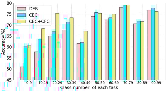
Figure 1.
Model performance on each task with different auxiliary loss after finishing training the last task on ImageNet100-B0 of 10 steps. We compare the accuracy of the two proposed contrastive auxiliary losses (CEC and CFC) and DER. The x axis shows the class ID for each task.
Moreover, the auxiliary loss forces new modules to collapse all old classes into a single category, which limits their ability to distinguish among old classes. Additionally, the imbalance between old and new classes allows the new-task feature extractor to dominate, biasing the model toward the new classes and causing it to misclassify samples from old classes—a phenomenon we term feature bias. While the knowledge of old classes is consolidated in the corresponding modules, this consolidation does not effectively translate into the new modules’ learning process.
A key challenge is how to effectively coordinate multiple feature extractors and integrate them into a unified model to mitigate catastrophic forgetting and enhance new task learning. By leveraging the consolidated knowledge from previous tasks embedded in old modules, we can enhance the new modules’ ability to better distinguish the features of different classes. We propose using asymmetric contrastive loss to not only aid in learning new tasks but also endow new modules to categories in old tasks, thus reducing feature confusion. Our main contributions are as follows:
- We reveal that simply freezing feature extractors fails to prevent forgetting in dynamically expandable networks—an overlooked limitation in existing research. Through in-depth analysis, we identify key factors shaping the stability–plasticity trade-off, demonstrating that widely used auxiliary losses and feature bias arising from the imbalance between old and new classes are major contributors to catastrophic forgetting.
- We introduce two novel asymmetric contrastive auxiliary losses: current feature contrastive loss (CEC loss) and cross feature contrastive loss (CFC Loss) as alternatives to the traditional auxiliary loss. These losses help the model achieve a better balance between plasticity and stability. Our approach integrates seamlessly with models that employ an auxiliary loss. We propose learning adjustable parameters to mitigate feature bias, ensuring that the corresponding modules maintain their dominance when handling their respective tasks.
- Our approach significantly enhances accuracy on three benchmarks compared to baseline methods, achieving state-of-the-art performance on the ImageNet benchmark. Furthermore, it offers substantial benefits to other methods such as DyTox and MCG, despite their differing network structures (ResNet and ViT) and methodologies.
2. Related Works
Continual learning aims to learn new tasks while mitigating catastrophic forgetting on old tasks. Elastic weight consolidation (EWC) [8] introduces a regularization term, limiting the modification of parameters crucial for old tasks to prevent catastrophic forgetting. Ref. [9] aim to mitigate catastrophic forgetting by imposing constraints on network parameters.
Knowledge distillation [10] is another widely used technique in incremental learning [11,12,13]. Ref. [14] augments the features of rehearsal samples at each layer for rehearsal-based methods.
Sample-imbalance between old and new categories often biases the classifier toward the latter. Several methods [12,15,16,17,18,19] explicitly address this bias. Dongwan Kim [20] proposed analytical tools for quantifying the stability–plasticity trade-off of learned features.
Single-extractor models often struggle to retain high accuracy under continual learning. AANets [21] and DualNet [2] used two feature extractors to achieve a better stability–plasticity trade-off. However, fully eliminating catastrophic forgetting with only two extractors remains challenging. Dynamically expandable networks allocate a fresh module—such as a feature extractor or task token—for every task while freezing all prior modules [6,22,23,24]. DER [4] dynamically expands the network and employs an auxiliary loss to guide each new extractor toward the current task. DyTox [5] instead appends a task-specific token per task within a Transformer backbone. SEED [25] trains multiple networks in which several tasks share one extractor while discarding old samples. DNE [7] utilizes dense connections between the intermediate layers of task expert networks, employing feature sharing and reusing to facilitate knowledge transfer from old to new tasks. MCG [6] adds a gating network that predicts the task identity and selects the most relevant extractor at inference time. Ref. [26] introduces a data-augmentation scheme shown to alleviate forgetting.
Contrastive learning [27,28,29] formulates pretext tasks on unlabeled data so that a network learns richer representations. Such representations transfer readily to downstream tasks. Supervised contrastive learning [30] extends the self-supervised objective to fully supervised settings. Co2L [31] shows that contrastively learned representations exhibit greater robustness to catastrophic forgetting. Ref. [32] propose maximizing mutual information online to combat forgetting. Ref. [33] combines supervised and self-supervised contrastive losses during pre-training to improve few-shot class-incremental learning.
Recent work leverages pre-trained models—such as Vision Transformers (ViT) [34], and introduces prompt-based strategies for incremental learning [35,36,37,38,39,40,41]. Ref. [42] expands the subspace with an adapter for each new task in pre-trained models.
3. Methodology
3.1. Problem Setup
In class-incremental learning, a model learns a sequence of tasks . For each task , there is a dataset that contains training examples, and their labels . contains classes, because the class sets are disjoint, the total number of classes is . After training on a task, a memory buffer retains a small number of samples to help the model mitigate forgetting. The memory buffer contains samples from previous tasks. The data available for the current training session is represented by . Let denote the module added at step i. Given an input x, it outputs a feature vector is , where d is the embedding dimension.
Dynamically expandable networks (DENs). When learning a new task, DENs augments the model with a new module, which can be a feature extractor or a task token. Previous modules are frozen to preserve their learned information. The features or embeddings processed by each module are then fed into a classifier. As the specific implementations of the DENs framework, DER adds a new feature extractor for each new task, and previous feature extractors are frozen. The concatenated features are then sent to the task-specific classifier at step t. DyTox [5] adds a new task token for each task. Each task-specific embedding from the task attention block is fed to task-specific classifiers. MCG [6] uses DER as its baseline and further incorporates additional feature extractors. For each task, it computes multiple centers so that, during testing, the weights are derived by comparing the similarity between a sample and each task center. These weights are then used to amplify the contribution of the most relevant feature extractor.
Auxiliary loss. To enable the newly added feature extractor to specifically focus on task and effectively distinguish between new and old tasks, DER uses auxiliary loss to train . An auxiliary classifier is used to solve a -way classification problem on , treating all previously learned classes as one class. is the class number in . Auxiliary loss can help DER improve both average accuracy and last step accuracy by at least [4], and is widely used in DyTox and MCG.
3.2. Rethinking the Stability–Plasticity Dilemma
DENs add a fresh module for every incoming task and freeze earlier modules to curb forgetting. However, our findings indicate that DENs still suffer from catastrophic forgetting.
Catastrophic forgetting in early tasks. After training on all tasks, we observe a substantial performance drop for early tasks in the final model configuration for DER. As shown in Figure 1, after completing training on 10 tasks in ImageNet100-B0S10, a significant degradation in performance is evident, with an accuracy gap exceeding between task and . We attribute this primarily to the auxiliary loss’s inadequate utilization of old task information and the feature bias arising from the imbalance between new and old class samples.
Feature bias in DENs. The data imbalance problem arises during the training of the new task, where the number of samples of new classes in is greater than the samples of old classes in memory . This imbalance leads to a bias in the model, favoring the classification of inputs as new classes. Given that the modules corresponding to the old tasks have been frozen, this dominance is due to the features extracted by the new feature extractor. As illustrated in Figure 2, following the training of 10 tasks on CIFAR100-B0 with DER. For each task , features extracted by exhibit significantly higher norms than those for any other task extracted by , and higher than those for extracted by any other extractor , where .
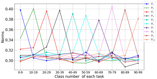
Figure 2.
Task-specific feature norm bias. The plot reports the mean feature norm for each task when its samples are fed through every DER feature extractor on CIFAR-100 B0S10. The x axis lists the class indices belonging to each task. Y axis means feature norm for each task.
Consequently, the new module focuses on the current task, and dominates in the model, leading to the catastrophic forgetting problem. Although this specialization is expected, it risks under-utilizing cross-task knowledge. These observations emphasize the critical need for strategies that more effectively balance the training influence between new and old tasks, aiming to mitigate feature bias.
Auxiliary loss hurts stability. Auxiliary loss helps the new module focus on learning the new task. However, while this approach may reduce the complexity of the feature space, it inadvertently increases confusion among old task classes. Specifically, the auxiliary loss fails to effectively enhance intra-class compactness and inter-class separation, leading to a degradation in discriminative ability among classes. Data imbalance amplifies the problem: the new-task module dominates, causing accuracy on earlier tasks to plummet. By design, the auxiliary loss does not directly address the need to maintain robust feature representations for old tasks, thereby undermining the stability of the model’s learning over time.
Auxiliary loss influences plasticity. During training, the auxiliary loss deliberately avoids distinguishing the classes from previous tasks so that the new feature extractor can concentrate on the current task. This blurring of distinctions among old classes can degrade the model’s capacity to recognize the unique characteristics of each class, leading to a diminished ability to effectively adapt and apply learned insights to new classes. Consequently, while auxiliary loss helps in mitigating interference from old tasks, it might compromise the nuanced understanding needed for new tasks, thus affecting the plasticity. Following the completion of each task , we assess the impact of auxiliary loss on the plasticity of each module associated with its corresponding task . After training task and obtaining N frozen modules , we evaluate the plasticity of each module by training a new classifier solely with for classifying the corresponding task . This setup constitutes a -way classification problem, where is the number of classes in task .
As depicted in Figure 3a, for the initial 10 classes of CIFAR100, the classification accuracy of the two methods is comparable. However, as the number of previously learned classes grows, the auxiliary loss begins to negatively impact the ability of module to effectively learn its corresponding task , when compared to CEC loss. Figure 3b illustrates that on ImageNet-1000, CEC loss consistently outperforms auxiliary loss.
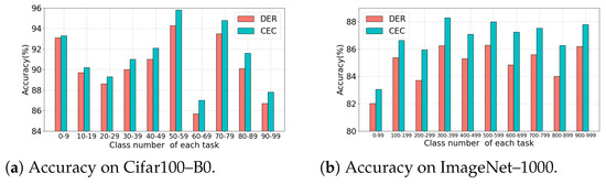
Figure 3.
Test accuracy of each task . When finishing learning N tasks (DER means training with auxiliary loss, CEC means using our proposed CEC loss to replace the auxiliary loss used in DER for training the new feature extractor), we obtain N feature extractors corresponding to N tasks. Subsequently, We use the frozen feature extractor and corresponding task data to train a new classifier (number of categories is ). We use the frozen feature extractor and new classifier to test .
These observations suggest that, while auxiliary loss facilitates easier learning for new tasks, it does so at the cost of impairing the model’s ability to accurately recall information from previously learned tasks, and affecting the new module’s plasticity. To mitigate these issues, it is crucial to develop strategies that not only balance the learning between new and old tasks but also fully leverage the existing knowledge from old tasks to support new task learning. This approach will enhance feature separation and compactness across all classes, thereby reducing forgetting.
3.3. Asymmetric Contrastive Auxiliary Loss
We therefore propose two asymmetric contrastive auxiliary losses for DENs: Current feature contrastive Loss (CEC loss) and cross-feature contrastive loss (CFC loss). These losses aim to enhance the network’s capability to retain knowledge from previously learned tasks while effectively learning new tasks.
As illustrated in Figure 4, when the model undertakes a new task at step t, a corresponding new module is introduced. Previous modules are frozen to prevent interference from subsequent learning processes.
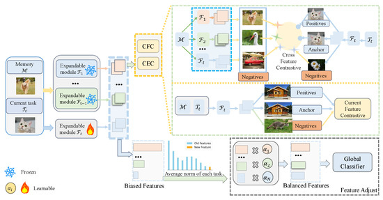
Figure 4.
Overview of our asymmetric contrastive auxiliary loss and feature adjustment. This figure illustrates the two-stage process when the model encounters a new task . New module (feature extractor or task tokens) will be added to the model. We use the cross feature contrastive loss (CFC) and current feature contrastive loss (CEC) to help learn more discriminative representations (Stage 1). Both CEC and CFC can be used in feature extractors or task tokens. After finishing the training of the feature extractors, we introduce adjustable parameters for each feature extractor to fine-tune the weight of each feature (Stage 2).
Current feature contrastive loss (CEC). The CEC loss is engineered to refine the representation of the current task by leveraging both new and old task samples, thereby enhancing intra-class compactness and inter-class separation within the new module. This not only improves the plasticity of the module with respect to new tasks but also equips it to better differentiate between classes from earlier tasks.
When training on a new task , the module processes a batch of N samples from the current task combined with samples from the memory buffer . Two data augmentation techniques are applied to produce a total of examples. The CEC loss trains the new module to discriminate between the current task and samples from . The features generated by are transformed into a projected vector by a two-layer perceptron projector . The CEC loss is as follows:
where represents the set of indices corresponding to samples of the same class as , j(j ≠ i)( = )}. is a positive scalar temperature parameter. By using Equation (1), learns to distinguish each class from both the old and new tasks. Old samples obtained from can serve as anchors to aid in learning to distinguish them from other classes. This is particularly beneficial for the model in mitigating the forgetting of old classes.
Cross-feature contrastive loss (CFC). During the training of old tasks, current task is not visible to modules , which were trained on previous tasks. As a result, struggle to differentiate the features related to . Features of derived from are ineffectual, offering no aid in learning . However, as have accumulated valuable knowledge from past tasks, this existing knowledge can be harnessed to enhance the learning capabilities of . Cross-feature contrastive loss (CFC) leverages features from old tasks preserved in to aid in effectively distinguishing between old and new tasks, thus helping to establish robust decision boundaries. This will enhance the model’s generalization capabilities across tasks.
The operational mechanism of the CFC loss involves projecting features from both old and new tasks into a shared feature space where they can be directly compared. Features from old tasks stored in the memory buffer , processed by , are projected by a shared projector , denoted by . Similarly, the features from the new module , corresponding to all available samples are also projected and denoted by . The combined set of features, , serves as the basis for the contrastive learning process:
The projector is shared by CEC loss and CFC loss, and will be discarded once the specific task training is complete.
Total loss for learning new modules. Following DER, we concatenate the features from all modules, and the concatenated features will be sent to the classifier for DER(For DyTox, following DyTox, we feed the embeddings to correspond classifier). Concatenated features are recorded as . The classifier is recorded as . Cross-entropy loss is used on the current task data and memory buffer as follows:
The overall loss for training is
where and are the hyper-parameters, and when the model learns the first task.
3.4. Feature Adjustment
After obtaining modules at stage 1, we next address the feature bias problem at stage 2. Due to data imbalance, both the module and the classifier tend to be biased toward the new task. The frozen modules store knowledge for the previous corresponding task . Fine-tuning the feature extractor on balanced datasets will impact the model’s performance. For solving the features bias problem, we introduce learnable parameters for each module , which is optimized to ensure balanced representation across tasks. These parameters can be adjusted to determine suitable weights for adapting to the entire task. We then concatenate the weighted features as follows:
All feature modules remain frozen so that their knowledge is preserved. Following DER, we then sample-balanced datasets from both the current task and the memory buffer , ensuring equitable representation across all classes. We re-train a fresh classifier with temperature-scaled cross-entropy (temperature ) while jointly learning .
Figure 5 illustrates the impact of our feature adjustment mechanism. Prior to adjustment, the feature norms of earlier tasks are significantly larger than those of later tasks, indicating an imbalance. Our feature adjustment (F.A.) mechanism reduces the norms of earlier tasks while increasing those of later tasks, resulting in a more balanced representation across all tasks and effectively mitigating the imbalance.
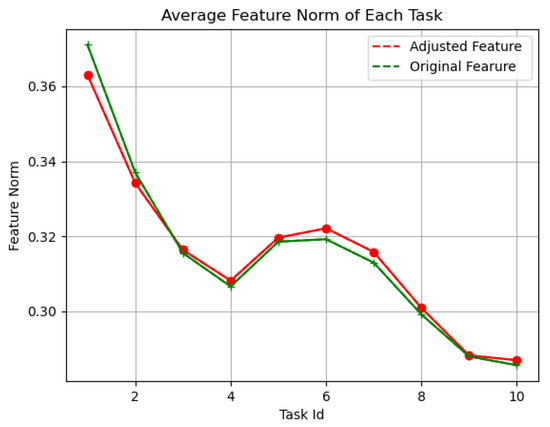
Figure 5.
Average feature norm of each task. Green line is original feature. Red line is feature norm adjusted by feature adjustment.
4. Experiments
This section evaluates the proposed method on three widely used benchmarks—CIFAR-100, ImageNet-100, and ImageNet-1000—under multiple class-incremental settings.
4.1. Setup
Datasets. ImageNet-1000 consists of 1000 classes with approximately 1.2 million training images and 50,000 validation images. ImageNet-100 is the 100-class subset. CIFAR100 includes 32 × 32 pixel color images across 100 classes, with 50,000 training images and 10,000 evaluation images.
Benchmarks. We follow standard splits on ImageNet-100, ImageNet-1000, and CIFAR-100. For all settings, we use the same class order as DER for ImageNet-1000 for fairness.
- (1).
- On ImageNet100 B0, the first task includes 10 classes, with each subsequent task adding 10 classes; the task size is 10, and the memory size is 2000.
- (2).
- On ImageNet100 B50, the first task has 50 classes, and each new task will add 5 classes, whilst the task size is 11. Each class will preserve 20 samples.
- (3).
- On ImageNet1000 B0, the first task has 100 classes, each task will add 100 classes, and task size is 10. The memory size is 20,000.
For CIFAR100, we evaluate the first task with 5, 10, 20 classes, and each subsequent task will add 5, 10, 20 classes, respectively, and the task size is 20, 10, 5, respectively. Memory size is 2000 examples in these settings.
In these experiments, we use herding selection strategy following DER to select samples to build .
Implementation Details. Our implementation is based on PyTorch 1.10.2. Following DER, we adopt the same network structure for the feature extractor . Specifically, for CIFAR100, we employ a modified ResNet-18 as the feature extractor, while for ImageNet-100 and ImageNet-1000, we utilize the standard ResNet-18. We use SGD as optimizer, and the learning rate is , momentum is , and weight decay is 0.0005. For CIFAR100, the batch size is 128. For ImageNet-100 and ImageNet-1000, the batch size is 256. Following [30], the temperature is fixed at .
The projector head uses the configuration of [30]. The output size of projector is 128 for all experiments. After completing each task, the projector is discarded. No projector is needed during testing. For the temperature parameter , we fully adhere to the settings used in DER [4], maintaining consistency by setting for CIFAR-100 and for ImageNet. In comparison to DER, only the same number of variables as the feature extractor is added.
Evaluation metrics. We report last-step and average accuracy. For ImageNet-100 and ImageNet-1000, we evaluate the top-1 and top-5 accuracy. Following the methodologies used by DER and DyTox, we calculated several key performance metrics: backward transfer (BWT), forward transfer (FWT), average accuracy, last step accuracy, and forgetting.
denotes the mean accuracy on all classes learned before task . is defined as the accuracy on Task after the completion of task .
FWT. Following GEM [43] and DER [4], We calculate the FWT as follows:
is the test accuracy obtained by model trained on available data with only cross-entropy loss at random initialization.
BWT. Following GEM [43] and DER [4], we calculate the BWT as follows:
Avg. The average accuracy is average accuracy of each step after finishing the last task T:
Last. Last step accuracy is defined as the accuracy measured on the entire test set after all training on the final task has been completed.
Comparative methods. We compare our method with iCaRL [11], BiC [16], WA [17], DER [4], DyTox [5], FOSTER [22], BEEF [23], MCG [6].
4.2. Evaluation on ImageNet-100
Table 1 top shows the test accuracy on ImageNet-100-B0. Compared to the baseline method DER, our method improves the last step accuracy from to . Average accuracy rises from to . Compared with SOTA methods MCG [6], our model has million fewer parameters, and the last step accuracy of top-1 accuracy is higher than MCG [6]. For top-5 accuracy, our method achieves higher average accuracy than the SOTA method. Our method achieves higher accuracy for the last step accuracy. Table 1 bottom shows that our method outperforms DER by in average accuracy, surpassing the MCG by in average accuracy on ImageNet-100-B50. Figure 6 illustrates the accuracy of each step and ImageNet-100.

Table 1.
Test accuracy on ImageNet-100 and ImageNet-1000 datasets. Top table is the result on ImageNet-100-B0 and ImageNet-1000-B0. The bottom table is the result on ImageNet-100-B50. Results of comparison methods come from [4,5,6]. DyTox [5] has an erratum regarding distributed memory on their official GitHub repository. The results of SEED [25] are taken from their paper, where old samples are not retained. #pcount means the average number of parameters when testing over step, calculated in millions. Average accuracy is recorded as Avg (%). Last step accuracy is recorded as Last (%). Bold values indicate the best performance.
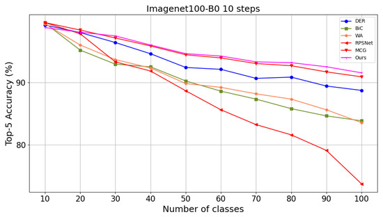
Figure 6.
Comparison of Top-5 accuracy at each step with other methods on ImageNet100-B0S10.
As shown in Figure 7, we use t-SNE [44] to visualize the feature distributions. The left plot presents the results of the baseline DER method, where features of old task classes appear scattered and less compact, indicating weaker retention of old task representations. In contrast, the right plot highlights the results of our proposed method, where features form more distinct clusters, demonstrating the better preservation of old task boundaries and improved feature separability.
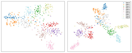
Figure 7.
t-SNE [44] visualization of the test set for ImageNet100B0S10 using the first task for illustration. The star symbols denote the prototypes of each class. The left plot presents the visualization of the baseline DER method, while the right plot showcases the results achieved with our proposed method.
4.3. Evaluation on ImageNet-1000
Table 1 top shows the test accuracy on ImageNet-1000-B0. Our method achieves state-of-the-art performance on the ImageNet-1000-B0 benchmark. Compared with baseline method DER, our method improves the last step accuracy from to . The average accuracy improves from to . Compared with the SOTA method, we use 11.2 million fewer parameters than the SOTA method. Our method outperforms the SOTA method by about for the last step top-1 accuracy, and the average accuracy can be higher than the SOTA method by about . For the last step accuracy of top-5, our method is higher than the SOTA method.
4.4. Evaluation on CIFAR100
Table 2 presents the results on CIFAR-100. Compared with the baseline method DER, our method demonstrates improved accuracy across three settings. In the CIFAR-100-B0 10-step setting, the last-step accuracy increases from to . For the 20-step setting, our method boosts the last-step accuracy from to . Our method also enhances the average accuracy from to . In the 5-step setting, our method improves the accuracy from to . Compared with state-of-the-art methods such as MCG, our approach utilizes approximately 11.2 million fewer parameters while achieving competitive results. Figure 8 illustrates the accuracy of each step on CIFAR-100.
Table 2.
Results on CIFAR100-B0, averaged over three different class orders. Results of the comparison method come from MCG [6], DyTox [5], and DER [4]. #pcount means the average number of parameters when testing over step, calculated in millions. Average accuracy is recorded as Avg (%). Last step accuracy is recorded as Last (%). MCG uses RandAugment when training CIFAR100. In this table, our method did not utilize RandAugmentation.
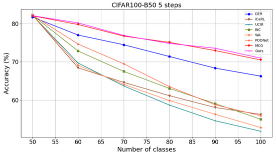
Figure 8.
Comparison of accuracy at each step with other methods on CIFAR100-B50S5.
RandAugment. Following the approach of MCG [6], we employ RandAugment, as depicted in Table 3, Table 4 and Table 5. On CIFAR100-B0S10, our method achieves a last-step accuracy that is higher by compared to MCG. By implementing RandAugment, the last-step accuracy increases from to . Table 5 presents the results on CIFAR100-B50, where the first task includes 50 classes, and each subsequent task adds 25 and 10 classes, respectively. Utilizing RandAugment, we achieve higher accuracy on CIFAR100 than MCG.
Table 3.
Results on CIFAR100-B0S10 Order2. MCG [6] trains gates using DER’s auxiliary loss. We replace the auxiliary loss with our losses (CEC. and CFC.), while keeping everything else unchanged, represented as “MCG + Ours” in the table. MCG uses RandAugment when training CIFAR100. “Ours + RA” indicates that we use RandAugment in our methods. The results of MCG are obtained by running their official open source code. #pcount means the average number of parameters when test over step, calculated in millions. Bold values indicate the best performance.
Table 4.
Results on CIFAR100-B0S20. MCG [6] uses RandAugment when training CIFAR100. “Ours + RA” indicates that we use RandAugment in our methods. #pcount means the average number of parameters when test over step, calculated in millions. Results of MCG is reported in their paper. Bold values indicate the best performance.
Table 5.
Results on CIFAR100-B50. MCG [6] uses RandAugment when training CIFAR100. “Ours + RA” indicates that we use RandAugment in our methods. #pcount means the average number of parameters when test over step, calculated in millions. Result on CIFAR100-B50, averaged over three different class orders. The results for MCG are sourced from their published paper.
4.5. Ablation Study
We conduct an ablation study on ImageNet100-B0S10 to analyze the effect of each component, as shown in Table 6. Using only improves the last step accuracy from to . Feature adjustment further enhances the accuracy to . With the assistance of and , the last step accuracy improves to . Feature adjustment is beneficial for DER, improving the last step accuracy from to .
Table 6.
Ablation study. Aux. denotes the auxiliary loss used in DER. F.A. stands for feature adjustment. A checkmark (✓) indicates that the corresponding component is used, while a cross (×) indicates it is not used.
To further elucidate the impact of our method on plasticity and stability, we calculated the backward transfer (BWT) for representation, and forward transfer (FWT) for representation [4]. Our results, presented in Table 7, demonstrate that our method significantly enhances the model’s ability to resist forgetting, CEC contributes positively to both plasticity and stability. On the other hand, the CFC markedly improves stability by effectively distinguishing between the features of new and old tasks. However, CFC may slightly constrain plasticity by rigidly separating task features. Our method achieves better a performance by balancing plasticity and stability.
Table 7.
BWT and FWT on Imagent100-B0S10.
4.6. Effects of Auxiliary Loss
To assess the effects of auxiliary losses on the interaction between new and old tasks, we compare the performance of DER using auxiliary loss and our proposed losses in predicting task ID, as illustrated in Figure 9. The comparison reveals that our proposed losses significantly enhance the ability to maintain task boundaries and reduce detrimental impacts on previously learned tasks. Figure 10 shows that, while our losses start slightly worse, they progressively reduce interference with prior tasks.
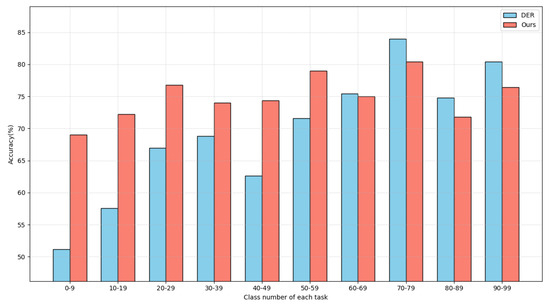
Figure 9.
Predicting task ID. Model performance in predicting task ID with different auxiliary loss for DER after having finished training the last task on ImageNet100-B0 of 10 steps. “Ours” refers to training DER using CEC and CFC loss. The abscissa represents the number of the class in the task.
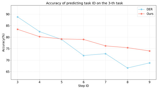
Figure 10.
Predicting task ID. Model performance in predicting task ID on the third task with different auxiliary loss after training each task on ImageNet100-B0 from step three to the last step. We compare the accuracy of the contrastive auxiliary losses and DER. “Ours” refers to training the model using CEC and CFC loss. The abscissa represents the step of current task.
4.7. Sensitive Study of Hyperparameters
We study the sensitivity to and , detailed results of which appear in Table 8 and Table 9. We use values of 0.9 and 0.7, respectively.
Table 8.
Sensitive study of for CEC loss.
Table 9.
Sensitive study of , is fixed at .
4.8. Computational and Parameter Overhead
In DER, a separate feature extractor is added for each task, making feature extraction the dominant runtime cost (30 ms per iteration) and incurring an additional 25 ms for each new extractor. In contrast, computing CEC and CFC adds merely 1.1 ms per training iteration. Both losses are disabled at inference, so runtime speed is unaffected. The feature-adjustment step in DER’s second stage merely scales each extractor’s output by a learned scalar, and our lightweight projector is instantiated only for the newly added extractor and removed after training, resulting in negligible parameter overhead.
4.9. Memory Size Setting
Table 10 reports results with memory budgets of 500, 1000 and 2000 exemplars. As expected, larger buffers yield higher accuracy.
Table 10.
Impact of memory size on performance.
4.10. Evaluation on DyTox
DyTox proposes a transformer architecture-based model with shared encoders and decoders across all tasks. A task token is added for learning each corresponding task. DyTox applies task attention in the final Transformer block only. Each task-specific embedding from the task attention block is fed to task-specific classifiers. DyTox uses cross-entropy loss, auxiliary loss, and additionally, a distillation loss.
Implementation on DyTox. For DyTox, we only replaced the auxiliary loss used in DyTox with our proposed contrastive loss. Additionally, we introduced a projector during training, which is discarded after training. We use the task tokens from the last task attention block to calculate the CEC and CFC loss.
Results on DyTox. We evaluated our contrastive loss on DyTox, which has corrected its results on their official GitHub repository for the use of distributed memory. For consistency and fairness, all experiments detailed in Table 11 were conducted under the distributed memory setting using two 3090 Ti GPUs. DyTox uses task-specific classifiers, so feature adjustment will not be utilized.
Table 11.
Ablation study on CIFAR100B0-10 for DyTox. The first row is obtained by running their official open source code. DyTox [5] corrected their result on their offical GitHub repository for using the distributed memory. All results in this table are with distributed memory. Aux. denotes the auxiliary loss used in DyTox.
As shown in Table 11, with the help of CEC and CFC loss, the average accuracy on CIFAR100 improves from to , and the last step accuracy improves from to .
Although DER (CNN backbone) and DyTox (ViT backbone + task tokens) introduce different per-task modules, our CEC and CFC losses improve both models, confirming that the two losses are architecture-agnostic. By injecting old-task information during new-task training, CEC and CFC sharpen the separation between task-specific modules while preserving the stability of previously learned ones.
Task tokens distance. DyTox reported that auxiliary loss enhances the diversity among task tokens by increasing the minimal Euclidean distance between them by . Following DyTox, we compared the task tokens distance obtained using various loss, as shown in Table 11, the minimal Euclidean distance increases by with the help of CEC compared to the distance with auxiliary loss. This finding underscores that our loss function offers enhanced capability in effectively differentiating between task tokens, suggesting potential improvements in task-specific classifier performance.
We compared the accuracy of DyTox at each step using different loss functions on CIFAR-100B0S10, as illustrated in Figure 11. During the learning of the first 10 classes, the original DyTox method (using auxiliary loss) demonstrates accuracy comparable to our methods. However, as more tasks are learned, our methods show a clear accuracy advantage. The DyTox with CFC method maintains similar accuracy to the original DyTox in the early stages, but outperforms it as the number of tasks increases. CEC loss, in contrast, rapidly demonstrates a marked improvement in accuracy right from the early stages.
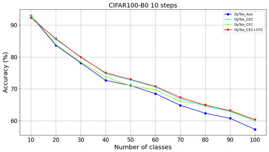
Figure 11.
Accuracy on CIFAR100B0S10 of DyTox with different auxiliary losses. DyTox_Aux, denotes the default DyTox method employing auxiliary loss.
As shown in Table 12, with the help of our loss, the average accuracy on ImageNet100B0S10 improves from to , the last step accuracy improves from to .
Table 12.
Results on ImageNet100-B0S10. DyTox [5] uses DER’s auxiliary loss. We replace the auxiliary loss with our losses (CEC. and CFC.), while keeping everything else unchanged, represented as “DyTox + Ours” in table. The result of DyTox is obtained by running their official open source code. DyTox corrected their result on their offical GitHub repository for using the distributed memory. All results in this table were conducted under the distributed memory setting using two 3090 Ti GPUs.
Forgetting and BWT. Following DyTox, we calculate the forgetting and backward transfer for representation, as shown in Table 11. We observed that compared to CEC, CFC demonstrates a more pronounced effect in mitigating BWT and reducing forgetting. This phenomenon is consistent within both DER and DyTox frameworks. CFC exhibits a stronger ability to resist forgetting than CEC.
4.11. Evaluation on MCG
Results on MCG. MCG [6] builds upon DER by assigning a new feature extractor for each task and freezing those from previous tasks to preserve knowledge. For each task, multiple centers are computed based on the feature distribution of its samples. A dedicated feature extractor is used to extract global features, which are then matched with the task-specific centers to compute dynamic weights. These weights adjust the contribution of each feature extractor, ensuring that the most relevant one plays a dominant role while minimizing the influence of less relevant ones.
We apply our contrastive loss to the MCG model [6]. We only replaced the auxiliary loss used in MCG with our proposed contrastive loss. As shown in Table 3, our method improves the average accuracy on CIFAR-100 from to , and the last-step accuracy increases from to . Similarly, as shown in Table 13 on ImageNet100-B0S10, our approach raises the average accuracy from to , and the last-step accuracy improves from to .
Table 13.
Results on ImageNet100-B0S10. MCG [6] trains gates using DER’s auxiliary loss. We replace the auxiliary loss with our losses (CEC. and CFC.), while keeping everything else unchanged, represented as “MCG + Ours” in the table. Results of MCG is reported in their paper. #pcount means the average number of parameters when test over step, calculated by millions. Bold values indicate the best performance.
5. Conclusions
We analyze the factors that govern stability–plasticity in dynamically expandable networks. Although auxiliary loss assists new modules in learning new tasks, it adversely affects both plasticity and stability. We address the stability–plasticity trade-off in dynamically expandable networks by replacing the standard auxiliary loss with an asymmetric contrastive auxiliary loss and by introducing learnable feature-weight adjustment to counter sample-induced feature bias, together yielding consistent accuracy gains on DER, DyTox, and MCG.
Author Contributions
Conceptualization, M.D. and R.L.; methodology, M.D.; software, M.D.; validation, M.D. and R.L.; formal analysis, M.D.; investigation, M.D.; resources, M.D.; data curation, M.D.; writing—original draft preparation, M.D.; writing—review and editing, R.L.; visualization, M.D.; supervision, M.D.; project administration, M.D. All authors have read and agreed to the published version of the manuscript.
Funding
This research received no external funding.
Data Availability Statement
The datasets used in this study are publicly available. CIFAR-10 can be accessed at https://www.cs.toronto.edu/~kriz/cifar.html (accessed on 7 August 2025) and ImageNet can be accessed at https://www.image-net.org/ (accessed on 7 August 2025).
Acknowledgments
The authors would like to thank our supervisor and colleagues for their valuable guidance and support throughout this work.
Conflicts of Interest
Author Rui Li was employed by the company “China Mobile (Hangzhou) Information Technology Co., Ltd.”. The remaining authors declare that the research was conducted in the absence of any commercial or financial relationships that could be construed as a potential conflict of interest.
References
- McCloskey, M.; Cohen, N. Catastrophic Interference in Connectionist Networks: The Sequential Learning Problem. In Psychology of Learning and Motivation; Elsevier: Amsterdam, The Netherlands, 1989; Volume 24, pp. 109–165. [Google Scholar]
- Pham, Q.; Liu, C.; Hoi, S. DualNet: Continual Learning, Fast and Slow. In Proceedings of the 35th Conference on Neural Information Processing Systems (NeurIPS), Virtual Event, 6–14 December 2021; pp. 16131–16144. [Google Scholar]
- McClelland, J.; McNaughton, B.; O’Reilly, R. Why There Are Complementary Learning Systems in the Hippocampus and Neocortex: Insights from the Successes and Failures of Connectionist Models of Learning and Memory. Psychol. Rev. 1995, 102, 419–457. [Google Scholar] [CrossRef] [PubMed]
- Yan, S.; Xie, J.; He, X. DER: Dynamically Expandable Representation for Class Incremental Learning. In Proceedings of the 34th IEEE/CVF Conference on Computer Vision and Pattern Recognition (CVPR), Nashville, TN, USA, 19–25 June 2021; pp. 3014–3023. [Google Scholar]
- Douillard, A.; Ramé, A.; Couairon, G.; Cord, M. DyTox: Transformers for Continual Learning with Dynamic Token Expansion. In Proceedings of the 35th IEEE/CVF Conference on Computer Vision and Pattern Recognition (CVPR), New Orleans, LA, USA, 19–24 June 2022; pp. 9285–9295. [Google Scholar]
- Cai, T.; Zhang, Z.; Tan, X.; Qu, Y.; Jiang, G.; Wang, C.; Xie, Y. Multi-Centroid Task Descriptor for Dynamic Class Incremental Inference. In Proceedings of the 36th IEEE/CVF Conference on Computer Vision and Pattern Recognition (CVPR), Vancouver, BC, Canada, 18–22 June 2023; pp. 7298–7307. [Google Scholar]
- Hu, Z.; Li, Y.; Lyu, J.; Gao, D.; Vasconcelos, N. Dense Network Expansion for Class Incremental Learning. In Proceedings of the 36th IEEE/CVF Conference on Computer Vision and Pattern Recognition (CVPR), Vancouver, BC, Canada, 18–22 June 2023; pp. 11858–11867. [Google Scholar]
- Kirkpatrick, J.; Pascanu, R.; Rabinowitz, N.; Veness, J.; Desjardins, G.; Rusu, A.; Milan, K.; Quan, J.; Ramalho, T.; Grabska-Barwinska, A.; et al. Overcoming Catastrophic Forgetting in Neural Networks. Proc. Natl. Acad. Sci. USA 2017, 114, 3521–3526. [Google Scholar] [CrossRef] [PubMed]
- Aljundi, R.; Babiloni, F.; Elhoseiny, M.; Rohrbach, M.; Tuytelaars, T. Memory Aware Synapses: Learning What (Not) to Forget. In Proceedings of the 15th European Conference on Computer Vision (ECCV), Munich, Germany, 8–14 September 2018; pp. 139–154. [Google Scholar]
- Hinton, G.; Vinyals, O.; Dean, J. Distilling the Knowledge in a Neural Network. arXiv 2015, arXiv:1503.02531. [Google Scholar]
- Rebuffi, S.A.; Kolesnikov, A.; Sperl, G.; Lampert, C. iCarl: Incremental Classifier and Representation Learning. In Proceedings of the 30th IEEE/CVF Conference on Computer Vision and Pattern Recognition (CVPR), Honolulu, HI, USA, 21–26 July 2017; pp. 2001–2010. [Google Scholar]
- Douillard, A.; Cord, M.; Ollion, C.; Robert, T.; Valle, E. PODNet: Pooled Outputs Distillation for Small-Tasks Incremental Learning. In Proceedings of the 16th European Conference on Computer Vision (ECCV), Virtual Event, 23–28 August 2020; pp. 86–102. [Google Scholar]
- Yu, L.; Twardowski, B.; Liu, X.; Herranz, L.; Wang, K.; Cheng, Y.; Jui, S.; van de Weijer, J. Semantic Drift Compensation for Class-Incremental Learning. In Proceedings of the 33rd IEEE/CVF Conference on Computer Vision and Pattern Recognition (CVPR), Virtual Event, 14–19 June 2020; pp. 6982–6991. [Google Scholar]
- Zheng, B.; Zhou, D.W.; Ye, H.J.; Zhan, D.C. Multi-Layer Rehearsal Feature Augmentation for Class-Incremental Learning. In Proceedings of the 41st International Conference on Machine Learning(ICML), Vienna, Austria, 21–27 July 2024. [Google Scholar]
- Hou, S.; Pan, X.; Loy, C.; Wang, Z.; Lin, D. Learning a Unified Classifier Incrementally via Rebalancing. In Proceedings of the 32nd IEEE/CVF Conference on Computer Vision and Pattern Recognition (CVPR), Long Beach, CA, USA, 16–20 June 2019; pp. 831–839. [Google Scholar]
- Wu, Y.; Chen, Y.; Wang, L.; Ye, Y.; Liu, Z.; Guo, Y.; Fu, Y. Large Scale Incremental Learning. In Proceedings of the 32nd IEEE/CVF Conference on Computer Vision and Pattern Recognition (CVPR), Long Beach, CA, USA, 16–20 June 2019; pp. 374–382. [Google Scholar]
- Zhao, B.; Xiao, X.; Gan, G.; Zhang, B.; Xia, S.T. Maintaining Discrimination and Fairness in Class Incremental Learning. In Proceedings of the 33rd IEEE/CVF Conference on Computer Vision and Pattern Recognition (CVPR), Virtual Event, 14–19 June 2020; pp. 13208–13217. [Google Scholar]
- Boschini, M.; Bonicelli, L.; Buzzega, P.; Porrello, A.; Calderara, S. Class-Incremental Continual Learning into the Extended Der-Verse. IEEE Trans. Pattern Anal. Mach. Intell. 2022, 45, 5497–5512. [Google Scholar] [CrossRef] [PubMed]
- He, J. Gradient Reweighting: Towards Imbalanced Class-Incremental Learning. In Proceedings of the 41st IEEE/CVF Conference on Computer Vision and Pattern Recognition (CVPR), Seattle, WA, USA, 17–21 June; pp. 16668–16677.
- Kim, D.; Han, B. On the Stability-Plasticity Dilemma of Class-Incremental Learning. In Proceedings of the 36th IEEE/CVF Conference on Computer Vision and Pattern Recognition (CVPR), Vancouver, BC, Canada, 18–22 June 2023; pp. 20196–20204. [Google Scholar]
- Liu, Y.; Schiele, B.; Sun, Q. Adaptive Aggregation Networks for Class-Incremental Learning. In Proceedings of the 34th IEEE/CVF Conference on Computer Vision and Pattern Recognition (CVPR), Nashville, TN, USA, 19–25 June 2021; pp. 2544–2553. [Google Scholar]
- Wang, F.Y.; Zhou, D.W.; Ye, H.J.; Zhan, D.C. FOSTER: Feature Boosting and Compression for Class-Incremental Learning. In Proceedings of the 17th European Conference on Computer Vision (ECCV), Tel Aviv, Israel, 23–27 October 2022; Springer: Berlin/Heidelberg, Germany; pp. 398–414. [Google Scholar]
- Wang, F.Y.; Zhou, D.W.; Liu, L.; Ye, H.J.; Bian, Y.; Zhan, D.C.; Zhao, P. BEEF: Bi-Compatible Class-Incremental Learning via Energy-Based Expansion and Fusion. In Proceedings of the The 11th International Conference on Learning Representations (ICLR), Kigali, Rwanda, 1–5 May 2023. [Google Scholar]
- Chen, X.; Chang, X. Dynamic Residual Classifier for Class Incremental Learning. In Proceedings of the 19th IEEE/CVF International Conference on Computer Vision (ICCV), Paris, France, 2–6 October 2023; pp. 18743–18752. [Google Scholar]
- Rypeść, G.; Cygert, S.; Khan, V.; Trzcinski, T.; Zieliński, B.; Twardowski, B. Divide and Not Forget: Ensemble of Selectively Trained Experts in Continual Learning. In Proceedings of the The 12th International Conference on Learning Representations (ICLR), Vienna, Austria, 7–11 May 2024. [Google Scholar]
- Ferdinand, Q.; Clement, B.; Papadakis, P.; Oliveau, Q.; Le Chenadec, G. Feature expansion and enhanced compression for class incremental learning. Neurocomputing 2025, 634, 129807. [Google Scholar] [CrossRef]
- He, K.; Fan, H.; Wu, Y.; Xie, S.; Girshick, R. Momentum Contrast for Unsupervised Visual Representation Learning. In Proceedings of the 33rd IEEE/CVF Conference on Computer Vision and Pattern Recognition (CVPR), Virtual Event, 14–19 June 2020; pp. 9729–9738. [Google Scholar]
- Grill, J.B.; Strub, F.; Altché, F.; Tallec, C.; Richemond, P.; Buchatskaya, E.; Doersch, C.; Avila Pires, B.; Guo, Z.; Gheshlaghi Azar, M.; et al. Bootstrap Your Own Latent: A New Approach to Self-Supervised Learning. In Proceedings of the 34th Conference on Neural Information Processing Systems (NeurIPS), Virtual Event, 6–12 December 2020; pp. 21271–21284. [Google Scholar]
- Chen, T.; Kornblith, S.; Swersky, K.; Norouzi, M.; Hinton, G. Big Self-Supervised Models are Strong Semi-Supervised Learners. arXiv 2020, arXiv:2006.10029. [Google Scholar]
- Khosla, P.; Teterwak, P.; Wang, C.; Sarna, A.; Tian, Y.; Isola, P.; Maschinot, A.; Liu, C.; Krishnan, D. Supervised Contrastive Learning. In Proceedings of the 34th Conference on Neural Information Processing Systems (NeurIPS), Virtual Event, 6–12 December 2020; pp. 18661–18673. [Google Scholar]
- Cha, H.; Lee, J.; Shin, J. Co2L: Contrastive Continual Learning. In Proceedings of the 18th IEEE/CVF International Conference on Computer Vision (ICCV), Virtual Event, 11–17 October 2021; pp. 9516–9525. [Google Scholar]
- Guo, Y.; Liu, B.; Zhao, D. Online Continual Learning Through Mutual Information Maximization. In Proceedings of the 39th International Conference on Machine Learning (ICML). PMLR, Baltimore, MD, USA, 17–23 July 2022; pp. 8109–8126. [Google Scholar]
- Ahmed, N.; Kukleva, A.; Schiele, B. OrCo: Towards Better Generalization via Orthogonality and Contrast for Few-Shot Class-Incremental Learning. In Proceedings of the 41st IEEE/CVF Conference on Computer Vision and Pattern Recognition (CVPR), Seattle, WA, USA, 17–21 June 2024. [Google Scholar]
- Dosovitskiy, A.; Beyer, L.; Kolesnikov, A.; Weissenborn, D.; Zhai, X.; Unterthiner, T.; Dehghani, M.; Minderer, M.; Heigold, G.; Gelly, S.; et al. An Image is Worth 16x16 Words: Transformers for Image Recognition at Scale. In Proceedings of the International Conference on Learning Representations (ICLR), Virtual Event, 3–7 May 2021. [Google Scholar]
- Wang, Z.; Zhang, Z.; Lee, C.Y.; Zhang, H.; Sun, R.; Ren, X.; Su, G.; Perot, V.; Dy, J.; Pfister, T. Learning to Prompt for Continual Learning. In Proceedings of the 35th IEEE/CVF Conference on Computer Vision and Pattern Recognition (CVPR), New Orleans, LA, USA, 19–24 June 2022; pp. 139–149. [Google Scholar]
- Wang, Z.; Zhang, Z.; Ebrahimi, S.; Sun, R.; Zhang, H.; Lee, C.Y.; Ren, X.; Su, G.; Perot, V.; Dy, J.; et al. DualPrompt: Complementary Prompting for Rehearsal-Free Continual Learning. In Proceedings of the 17th European Conference on Computer Vision (ECCV), Tel Aviv, Israel, 23–27 October 2022; Springer: Berlin/Heidelberg, Germany, 2022; pp. 631–648. [Google Scholar]
- Wang, Y.; Huang, Z.; Hong, X. S-Prompts Learning with Pre-Trained Transformers: An Occam’s Razor for Domain Incremental Learning. In Proceedings of the 36th Conference on Neural Information Processing Systems (NeurIPS), New Orleans, LA, USA, 28 November–9 December 2022. [Google Scholar]
- Smith, J.; Karlinsky, L.; Gutta, V.; Cascante-Bonilla, P.; Kim, D.; Arbelle, A.; Panda, R.; Feris, R.; Kira, Z. CODA-Prompt: COntinual Decomposed Attention-Based Prompting for Rehearsal-Free Continual Learning. In Proceedings of the 36th IEEE/CVF Conference on Computer Vision and Pattern Recognition (CVPR), Vancouver, BC, Canada, 18–22 June 2023; pp. 11909–11919. [Google Scholar]
- Wang, L.; Xie, J.; Zhang, X.; Huang, M.; Su, H.; Zhu, J. Hierarchical Decomposition of Prompt-Based Continual Learning: Rethinking Obscured Sub-Optimality. In Proceedings of the 37th Conference on Neural Information Processing Systems, New Orleans, LA, USA, 10–16 December 2023. [Google Scholar]
- Wang, R.; Duan, X.; Kang, G.; Liu, J.; Lin, S.; Xu, S.; Lü, J.; Zhang, B. AttriCLIP: A Non-Incremental Learner for Incremental Knowledge Learning. In Proceedings of the 36th IEEE/CVF Conference on Computer Vision and Pattern Recognition (CVPR), Vancouver, BC, Canada, 18–22 June 2023; pp. 3654–3663. [Google Scholar]
- Lu, H.Y.; Lin, L.K.; Fan, C.; Wang, C.; Fang, W.; Wu, X.J. Knowledge-guided prompt-based continual learning: Aligning task-prompts through contrastive hard negatives. Knowl.-Based Syst. 2025, 310, 113009. [Google Scholar] [CrossRef]
- Zhou, D.W.; Sun, H.L.; Ye, H.J.; Zhan, D.C. Expandable Subspace Ensemble for Pre-Trained Model-Based Class-Incremental Learning. In Proceedings of the 36th IEEE/CVF Conference on Computer Vision and Pattern Recognition (CVPR), Seattle, WA, USA, 17–21 June 2024. [Google Scholar]
- Lopez-Paz, D.; Ranzato, M. Gradient Episodic Memory for Continuum Learning. arXiv 2017, arXiv:1706.08840. [Google Scholar]
- Van der Maaten, L.; Hinton, G. Visualizing Data Using t-SNE. J. Mach. Learn. Res. 2008, 9, 2579–2605. [Google Scholar]


Disclaimer/Publisher’s Note: The statements, opinions and data contained in all publications are solely those of the individual author(s) and contributor(s) and not of MDPI and/or the editor(s). MDPI and/or the editor(s) disclaim responsibility for any injury to people or property resulting from any ideas, methods, instructions or products referred to in the content. |
© 2025 by the authors. Licensee MDPI, Basel, Switzerland. This article is an open access article distributed under the terms and conditions of the Creative Commons Attribution (CC BY) license (https://creativecommons.org/licenses/by/4.0/).