Sensitivity of High-Scale SUSY in Low Energy Hadronic FCNC

Abstract

We discuss the sensitivity of the high-scale supersymmetry (SUSY) at 10–1000 TeV in B⁰, B_s, K⁰ and D meson systems together with the neutron electric dipole moment (EDM) and the mercury EDM. In order to estimate the contribution of the squark flavor mixing to these flavor changing neutral currents (FCNCs), we calculate the squark mass spectrum, which is consistent with the recent Higgs discovery. The SUSY contribution in ϵ_K could be large, around 40% in the region of the SUSY scale 10–100 TeV. The neutron EDM and the mercury EDM are also sensitive to the SUSY contribution induced by the gluinosquark interaction. The predicted EDMs are roughly proportional to $\left|{ϵ}_K^{\text{SUSY}}\right|$. If the SUSY contribution is the level of $\mathcal{O}$ (10%) for ϵ_K, the neutron EDM is expected to be discovered in the region of 10⁻²⁸–10⁻²⁶ ecm. The mercury EDM also gives a strong constraint for the gluinosquark interaction. The SUSY contribution of ΔM_D is also discussed.

1. Introduction

Supersymmetry (SUSY) is one of the most attractive theories beyond the standard model (SM). Therefore, SUSY has been expected to be observed at the LHC experiments. However, no signals of SUSY have been discovered yet. The present searches for SUSY particles give us important constraints for SUSY. Since the lower bounds of the superparticle masses increase gradually, the squark and the gluino masses are supposed to be at a higher scale than 1 TeV [1–3]. On the other hand, the SUSY model has been seriously constrained by the Higgs discovery, in which the Higgs mass is 125 GeV [4–6]. Based on this theoretical and experimental situation, we consider the high-scale SUSY models, which have been widely discussed with a great deal of attention [7–22].

If the squark and slepton masses are at the high-scale $\mathcal{O}$ (10–1000) TeV, the lightest Higgs mass can be pushed up to 125 GeV, whereas SUSY particles are out of the reach of the LHC experiment. Therefore, the indirect search of the SUSY particles becomes important in the low-energy flavor physics [23–25].

The flavor physics is also on the a stage in light of LHCb data. The LHCb collaboration has reported new data of the CP violation of the B_s meson and the branching ratios of rare B_s decays [26–38]. For many years, the CP violation in the K and B⁰ mesons has been successfully understood within the framework of the standard model (SM), the so-called Kobayashi–Maskawa (KM) model [39], where the source of the CP violation is the KM phase in the quark sector with three families. However, a new physics has been expected to be indirectly discovered in the precise data of B⁰ and B_s meson decays at the LHCb experiment and the further coming experiment, Belle-II.

There are new sources of the CP violation if the SM is extended to the SUSY models. The soft squark mass matrices contain the CP violating phases, which contribute to the flavor changing neutral current (FCNC) with the CP violation [40]. Therefore, we can expect the SUSY effect in the CP violating phenomena. However, the clear deviation from the SM prediction has not been observed yet in the LHCb experiment [26–38]. Actually, we have found that the CP violation of B⁰ and B_s meson systems are suppressed if the SUSY scale is above 10 TeV [41]. On the other hand, the CKM fitter group presented the current limits on new physics contributions of $\mathcal{O}$ (10%) in B⁰, B_s and K⁰ systems [42]. They have also estimated the sensitivity to new physics in B⁰ and B_s mixing achievable with 50 ab⁻¹ of Belle-II and 50 fb⁻¹ of LHCb data. Therefore, we should carefully study the sensitivity of the high-scale SUSY to the hadronic FCNC.

In this work, we discuss the high-scale SUSY contribution to the B⁰, B_s and K⁰ meson systems. Furthermore, we also discuss the sensitivity to the D meson and the electric dipole moment (EDM) of the neutron and mercury. For these modes, the most important process of the SUSY contribution is the gluino-squark-mediated flavor changing process [43–58]. The CP violation of the K meson, ϵ_K, provides a severe constraint to the gluino-squark-mediated FCNC [59,60]. In addition, recent work has found that the chromo-electric dipole moment (cEDM) is sensitive to the high-scale SUSY [61]. It is noted that the upper-bound of the neutron EDM (nEDM) [62] gives a severe constraint for the gluino-squark interaction through the cEDM [63–68]. It is also remarked that the upper bound of the mercury EDM (HgEDM) [69] can give an important constraint [70].

In order to estimate the gluino-squark-mediated FCNC of the K, B⁰, B_s and D mesons, we work in the basis of the squark mass eigenstate with the non-minimal squark (slepton) flavor mixing. There are three reasons why the SUSY contribution to the FCNC considerably depends on the squark mass spectrum. The first one is that the GIM mechanism works in the squark flavor mixing, and the second one is that the loop functions depend on the mass ratio of the squark and gluino. The last one is that we need the mixing angle between the left-handed sbottom and right-handed sbottom, which dominates the ΔB = 1 decay processes. Therefore, we discuss the squark mass spectrum, which is consistent with the recent Higgs discovery. Taking the universal soft parameters at the SUSY breaking scale, we obtain the squark mass spectrum at the matching scale where the SM emerges, by using the renormalization group equations (REGs) of the soft masses. On the other hand, the 6 × 6 mixing matrix between squarks and quarks is taken to be free at the low energy.

In Section 2, we discuss the squark and gluino mass spectrum and the squark mixing. In Section 3, we present the formulation of the FCNC with ΔF = 2 in the K, B⁰, B_s and D meson systems together with nEDM and HgEDM. We present numerical results and discussions in Section 4. Section 5 is devoted to the summary. The relevant formulations are presented in Appendices A–D.

2. SUSY Spectrum and Squark Mixing

The low-energy FCNCs depend significantly on the spectrum of the SUSY particles, which depend on the model. As is well known, the lightest Higgs mass can be pushed up to 125 GeV if the squark masses are expected to be $\mathcal{O}$ (10) TeV. Therefore, let us consider the heavy SUSY particle mass spectrum in the framework of the minimal supersymmetric standard model (MSSM), which is consistent with the observed Higgs mass. The discussion of how to obtain the SUSY spectrum has been given in [71,72].

We outline how to obtain the SUSY spectrum in our work. The details are presented in Appendix A. At the SUSY breaking scale Λ, we write the quadratic terms in the MSSM potential as:

$$V_2=m_1^2{\left|H_1\right|}^2+m_2^2{\left|H_2\right|}^2+m_3^2\left(H_1\cdot H_2+h.c.\right)$$

(1)

Then, the Higgs mass parameter m² is expressed in terms of $m_1^2$, $m_2^2$ and tan β as:

$$m^2=\frac{m_1^2-m_2^2{\tan }^2\beta }{{\tan }^2\beta -1}$$

(2)

After running down to the Q₀ scale, in which the SM emerges, by the one-loop SUSY renormalization group equations (RGEs) [73], the scalar potential is the SM one as follows:

$$V_{SM}=-m^2{\left|H\right|}^2+\frac{\lambda }{2}{\left|H\right|}^4$$

(3)

Here, the Higgs coupling λ is given in terms of the SUSY parameters at the leading order as:

$$\lambda \left(Q_0\right)=\frac{1}{4}\left(g^2+{g^{\prime }}^2\right){\cos }^{2}2\beta +\frac{3h_t^2}{8{\pi }^2}{X}_t^2\left(1-\frac{X_t^2}{12}\right),X_t=\frac{A_t\left(Q_0\right)-\mu \left(Q_0\right)\cot \beta }{Q_0}$$

(4)

and h_t is the top Yukawa coupling of the SM. The parameters m₂ and λ run with the two-loop SM RGEs with the $\overline{\mathrm{MS}}$ scheme [74–76] down to the electroweak scale Q_EW = m_H and then give:

$$m_H^2=2m^2\left(m_H\right)=\lambda \left(m_H\right){\upsilon }^2$$

(5)

When m_H = 125 GeV is placed, λ(Q₀) and m² (Q₀) are obtained. This input constrains the SUSY mass spectrum of the MSSM. In our work, we take the universal soft breaking parameters at the SUSY breaking scale Λ as follows:

$$\begin{array}{l}{m}_{{\tilde{Q}}_i}\left(\mathrm{\Lambda }\right)=m_{{\tilde{U}}_i^c}\left(\mathrm{\Lambda }\right)=m_{{\tilde{D}}_i^c}\left(\mathrm{\Lambda }\right)=m_{{\tilde{L}}_i}\left(\mathrm{\Lambda }\right)=m_{{\tilde{E}}_{{}^i}^c}\left(\mathrm{\Lambda }\right)=m_0^2\left(i=1,2,3\right)\\ M_1\left(\mathrm{\Lambda }\right)=M_2\left(\mathrm{\Lambda }\right)=M_3\left(\mathrm{\Lambda }\right)=m_{1/2},m_1^2\left(\mathrm{\Lambda }\right)=m_2^2\left(\mathrm{\Lambda }\right)=m_0^2\\ A_U\left(\mathrm{\Lambda }\right)=A_{0yU}\left(\mathrm{\Lambda }\right),A_D\left(\mathrm{\Lambda }\right)=A_{0yD}\left(\mathrm{\Lambda }\right),A_E\left(\mathrm{\Lambda }\right)=A_{0yE}\left(\mathrm{\Lambda }\right)\end{array}$$

(6)

By inputting m_H = 125 GeV and taking the heavy scalar mass $m_{\mathscr{H}}\simeq Q_0$ (see Appendix A), we can obtain the SUSY spectrum for the fixed Q₀ and tan β. The details and numerical results are presented in Appendix A.

Let us consider the squark flavor mixing. As discussed above, there is no flavor mixing at Λ in the MSSM. However, in order to consider the non-minimal flavor mixing framework, we allow the off-diagonal components of the squark mass matrices at the 10% level, which leads to the flavor mixing of order 0.1. We take these flavor mixing angles as free parameters at low energies. Now, we consider the 6 × 6 squark mass matrix $M_{\tilde{q}}$ in the super-CKM basis. In order to move the mass eigenstate basis of squark masses, we should diagonalize the mass matrix by rotation matrix ${\mathrm{\Gamma }}_G^{(q)}$ as:

$$m_{\tilde{q}}^2={\mathrm{\Gamma }}_G^{\left(q\right)}{M}_{\tilde{q}}^2{\mathrm{\Gamma }}_G^{\left(q\right)†}$$

(7)

where ${\mathrm{\Gamma }}_G^{(q)}$ is the 6×6 unitary matrix, and we decompose it into the 3×6 matrices as ${\mathrm{\Gamma }}_G^{(q)}={\left({\mathrm{\Gamma }}_{GL}^{(q)},{\mathrm{\Gamma }}_{GR}^{(q)}\right)}^T$ in the following expressions:

$$\begin{array}{l}{\mathrm{\Gamma }}_{GL}^{\left(d\right)}=\left(\begin{array}{cccccc}{c}_{13}^L& 0& s_{13}^L{e}^{-{\varphi }_{13}^L}{c}_{\theta }& 0& 0& -s_{13}^L{e}^{-i{\varphi }_{13}^L}{s}_{\theta }{e}^{i\varphi }\\ -s_{23}^L{s}_{13}^L{e}^{i\left({\varphi }_{13}^L-{\varphi }_{23}^L\right)}& c_{23}^L& s_{23}^L{c}_{13}^L{e}^{-i{\varphi }_{23}^L}{c}_{\theta }& 0& 0& -s_{13}^L{c}_{23}^L{e}^{-i{\varphi }_{13}^L}{s}_{\theta }{e}^{i\varphi }\\ -s_{13}^L{c}_{23}^L{e}^{i{\varphi }_{13}^L}& -s_{23}^L{e}^{i{\varphi }_{23}^L}& c_{13}^L{c}_{23}^L{c}_{\theta }& 0& 0& -c_{13}^L{c}_{23}^L{s}_{\theta }{e}^{i\varphi }\end{array}\right)\\ {\mathrm{\Gamma }}_{GR}^{\left(d\right)}=\left(\begin{array}{cccccc}0& 0& s_{13}^R{s}_{\theta }{e}^{-i{\varphi }_{13}^R}{e}^{-i\varphi }& c_{13}^R& 0& s_{13}^R{e}^{-i{\varphi }_{13}^R}{c}_{\theta }\\ 0& 0& s_{23}^R{c}_{13}^R{s}_{\theta }{e}^{-i{\varphi }_{23}^R}{e}^{-i\varphi }& -s_{13}^R{s}_{23}^R{s}_{\theta }{e}^{-i\left({\varphi }_{13}^R-{\varphi }_{23}^R\right)}& c_{23}^R& s_{23}^R{c}_{13}^R{e}^{-i{\varphi }_{23}^R}{c}_{\theta }\\ 0& 0& c_{13}^R{c}_{23}^R{s}_{\theta }{e}^{-i\varphi }& -s_{13}^R{c}_{23}^R{e}^{i{\varphi }_{13}^R}& -s_{23}^R{e}^{i{\varphi }_{23}^R}& c_{13}^R{c}_{23}^R{c}_{\theta }\end{array}\right)\end{array}$$

(8)

where we use abbreviations $c_{ij}^{L,R}=\cos {\theta }_{ij}^{L,R},$$s_{ij}^{L,R}=\sin {\theta }_{ij}^{L,R},$c_θ = cos θ and s_θ = sin θ. Here, θ is the left-right mixing angle between ${\tilde{b}}_L$ and ${\tilde{b}}_R$, which is discussed in Appendix A. It is remarked that we take $s_{12}^{L,R}=0$ due to the degenerate squark masses of the first and second families, as discussed in Appendix A.

The gluino-squark-quark interaction is given as:

$${ℒ}_{\mathrm{int}}\left(\tilde{g}q\tilde{q}\right)=-i\sqrt{2}{g}_s{\displaystyle \sum _{\left\{q\right\}}{\tilde{q}}_i^{*}}\left(T^a\right)\overline{{\tilde{G}}^a}\left[{\left({\mathrm{\Gamma }}_{GL}^{\left(q\right)}\right)}_{ij}L+{\left({\mathrm{\Gamma }}_{GR}^{\left(q\right)}\right)}_{ij}R\right]q_j+h.c.$$

(9)

where $L=\left(1-{\gamma }_5\right)/2$, $R=\left(1-{\gamma }_5\right)/2$ and ${\tilde{G}}^a$ denotes the gluino field; qⁱ are three left-handed (i = 1, 2, 3) and three right-handed quarks (i = 4, 5, 6). This interaction leads to the gluino-squark-mediated flavor changing processes with ΔF = 2 and ΔF = 1 through the box and penguin diagrams.

The chargino (neutralino)-squark-quark interaction can be also discussed in a similar way.

3. FCNC of ΔF = 2

In our previous work [41], we have probed the high-scale SUSY, which is at the 10–50 TeV scale, in the CP violations of K, B⁰ and B_s mesons. It is found that ϵ_K is most sensitive to SUSY, even if the SUSY scale is at 50 TeV. The SUSY contributions for the time-dependent CP asymmetries of B⁰ and B_s with ΔB = 1 are suppressed at the SUSY scale of 10 TeV. Furthermore, the SUSY contribution for the b → sγ process is also suppressed, since the left-right mixing angle, which induces the chiral enhancement, is very small, as discussed in Appendix A. Therefore, we discuss the neutral meson mixing $P^0-{\overline{P}}^0$ (P⁰ = K, B⁰, B_s, D), which are FCNCs with ΔF = 2.

In those FCNCs, the dominant SUSY contribution is given through the gluino-squark interaction. Then, the dispersive part of meson mixing $M_{12}^{P^0}$ (P⁰ = K, B⁰, B_s) is written as:

$$M_{12}^{P^0}=M_{12}^{P^0,\mathrm{SM}}+M_{12}^{P^0,\text{SUSY}}$$

(10)

where $M_{12}^{q,\text{SUSY}}$ are given by the squark mixing parameters in Equation (8), and its explicit formulation is given in Appendices B and C.

At first, we discuss the ΔB = 2 process, that is the mass differences $\mathrm{\Delta }{M}_{B^0}$ and $\mathrm{\Delta }{M}_{B_s}$ and the CP-violating phases ϕ_d and ϕ_s. In general, the contribution of the new physics (NP) to the dispersive part $M_{12}^q$ is parameterized as:

$$M_{12}^{B_q}=M_{12}^{q,\mathrm{SM}}+M_{12}^{q,\mathrm{NP}}=M_{12}^{q,\mathrm{SM}}\left(1+h_q{e}^{2i{\sigma }_q}\right),\left(q=B^0,B_s\right)$$

(11)

where $M_{12}^{q,\mathrm{NP}}$ are the NP contributions. The generic fits for B⁰ and B_s mixing have given the constraints on (h_q, σ_q) [42], where it is assumed that the NP does not significantly affect the SM tree-level charged-current interaction, that is the absorptive part ${\mathrm{\Gamma }}_{12}^q$ is dominated by the decay $b\to c\overline{c}s.$ At present, the NP contributions h_q are 10%–35% and 15%–25%, depending on σ_q for B⁰ and B_s, respectively. Thus, we can expect the sizable NP contribution of $\mathcal{O}$ (20%). We will discuss whether the high-scale SUSY can fill in the magnitude of the present NP contribution of $\mathcal{O}$ (20%).

Next, we discuss the ΔS = 2 process, $\mathrm{\Delta }{M}_{K^0}$ and the CP-violating parameter in the K meson, ϵ_K. By the similar parametrization in Equation (11), the allowed region of (h_K, σ_K) has been estimated in [42]. The NP contribution is at least 50%, although there is the strong σ_K dependence. Therefore, it is important to examine carefully the CP violating parameter ϵ_K, which is given as follows:

$${ϵ}_K=e^{i{\varphi }_{ϵ}}\sin {\varphi }_{ϵ}\left(\frac{\mathrm{Im}\left(M_{12}^K\right)}{\mathrm{\Delta }{M}_K}+\xi \right),\xi =\frac{\mathrm{Im}{A}_0^K}{\mathrm{Re}{A}_0^K},{\varphi }_{ϵ}={\tan }^{-1}\left(\frac{2\mathrm{\Delta }{M}_K}{\mathrm{\Delta }{\mathrm{\Gamma }}_K}\right)$$

(12)

with $A_0^K$ being the isospin zero amplitude in K → ππ decays. Here, $M_{12}^K$ is the dispersive part of the $K^0-{\overline{K}}^0$ mixing, and ΔM_K is the mass difference in the neutral K meson. The effects of ξ ≠ 0 and φ_ϵ < π/4 give a suppression effect in ϵ_K, and it is parameterized as κ_ϵ and estimated by Buras and Guadagnoli [77] as:

$${\kappa }_{ϵ}=0.92\pm 0.02$$

(13)

In the SM, the dispersive part $M_K^{12}$ is given as follows,

$$\begin{array}{l}{M}_K^{12}=\langle K\left|{\mathscr{H}}_{\mathrm{\Delta }F=2}\right|\overline{K}\rangle \\ =-\frac{4}{3}{\left(\frac{G_F}{4\pi }\right)}^2{M}_W^2{\widehat{B}}_K{F}_K^2{M}_K\left({\eta }_{cc}{\lambda }_c^{2}E\left(x_c\right)+{\eta }_{tt}{\lambda }_t^{2}E\left(x_t\right)+2{\eta }_{ct}{\lambda }_c{\lambda }_{t}E\left(x_c,x_t\right)\right)\end{array}$$

(14)

where ${\lambda }_c=V_{cs}{V}_{cd}^{*}$, ${\lambda }_t=V_{ts}{V}_{td}^{*}$. The E(x)’s are the one-loop functions [78], and η_cc,tt,ct are the QCD corrections [77]. Then, $\left|{ϵ}_K^{\mathrm{SM}}\right|$ is given in terms of the Wolfenstein parameters λ, $\overline{\rho }$ and $\overline{\eta }$ as follows:

$${ϵ}_K^{\mathrm{SM}}={\kappa }_{ϵ}{C}_{ϵ}{\widehat{B}}_K{\left|V_{cb}\right|}^2{\lambda }^2\overline{\eta }\left({\left|V_{cb}\right|}^2\left(1-\overline{\rho }\right){\eta }_{tt}E\left(x_t\right)-{\eta }_{cc}E\left(x_c\right)+{\eta }_{ct}E\left(x_c,x_t\right)\right)$$

(15)

with

$$C_{ϵ}=\frac{G_F^2{F}_K^2{m}_K{M}_W^2}{6\sqrt{2}{\pi }^2\mathrm{\Delta }{M}_K}$$

(16)

Note that $\left|{ϵ}_K^{\mathrm{SM}}\right|$ depends on the non-perturbative parameter ${\widehat{B}}_K$ in Equation (15). Recently, the error of this parameter shrank dramatically in the lattice calculations [79]. In our calculation, we use the updated value by the flavor Lattice averaging group [80]:

$${\widehat{B}}_K=0.766\pm 0.010$$

(17)

Let us write down ϵ_K as:

$${ϵ}_K={ϵ}_K^{\mathrm{SM}}+{ϵ}_K^{\text{SUSY}}$$

(18)

where ${ϵ}_K^{\text{SUSY}}$ is induced by the imaginary part of the gluino-squark box diagram, which is presented in Appendices B and C. Since $S_{12}^{L(R)}$ vanishes in our scheme, ${ϵ}_K^{\text{SUSY}}$ is given in the second order of the squark mixing $S_{13}^{L(R)}\times S_{23}^{L(R)}$.

In addition to the above FCNC processes, the neutron EDM, d_n, arises through the cEDM of the quarks, $d_q^c$, due to the gluino-squark mixing [63–68]. By using the QCD sum rules, d_n is given as:

$$d_n=\left(0.79d_d-0.20d_u\right)+e\left(0.3d_u^C+0.59d_d^C\right)$$

(19)

where d_q and $d_q^c$ denote the EDM and cEDM of quarks $d_q^c$ defined in Appendix D. On the other hand, by using the chiral perturbation theory:

$$d_n=e\left(3.0d_u^C+2.5d_d^C+0.5d_s^C\right)$$

(20)

Therefore, the experimental upper bound [62]:

$$\left|d_n\right|<0.29\times {10}^{-25}\text{ecm}$$

(21)

provides us a strong constraint to the gluino-squark mixing.

The HgEDM can also probe the gluino-squark mixing [70]. The QCD sum rule approach gives [81]:

$$d_{Hg}=e\left(d_u^C-d_d^C+0.012d_s^C\right)\times 3.2\times {10}^{-2}$$

(22)

and the chiral Lagrangian method gives [82]:

$$d_{Hg}=e\left(d_u^C-d_d^C+0.0051d_s^C\right)\times 8.7\times {10}^{-3}$$

(23)

The experimental upper bound [69]:

$$|d_{Hg}|<3.1\times {10}^{-29}\text{ecm}$$

(24)

constrains the gluino-squark mixing.

At the last step, we discuss the charmsector, which is a promising field to probe for the new physics beyond the SM. The D⁰−D⁰ mixing is now well established [83] as follows:

$$x_D=\frac{\mathrm{\Delta }{M}_D}{{\mathrm{\Gamma }}_D}=\left(3.6\pm 1.6\right)\times {10}^{-3},y_D=\frac{\mathrm{\Delta }{\mathrm{\Gamma }}_D}{2{\mathrm{\Gamma }}_D}=\left(6.1\pm 0.7\right)\times {10}^{-3}$$

(25)

where ΔM_D and ΔΓ_D are the differences of the masses and the decay widths between the mass eigenstates of the D meson, respectively, and Γ_D is the averaged decay width of the D meson. Since the SM prediction of ΔM_D at the short distance is much suppressed compared with the experimental value due to the bottom quark loop, the SUSY contribution may be enhanced.

4. Results and Discussions

Let us estimate the SUSY contribution of the low-energy FCNC. We calculate the SUSY mass spectrum at Q₀ = 10, 50, 100, 1000 TeV and interpolate the each mass of the SUSY particle in the region of Q₀ = 10–1000 TeV. This approximation is satisfied within $\mathcal{O}$ (10%). Therefore, our numerical results should be taken with the ambiguity of $\mathcal{O}$ (10%). The mass spectrum at Q₀ = 10 TeV is presented in Appendix A. See [41,60] for the mass spectrum at Q₀ = 50 TeV.

Then, we have four mixing angles ${\theta }_{13}^{L(R)}$ and ${\theta }_{23}^{L(R)}$, five phase ${\varphi }_{13}^{L(R)}$, ${\varphi }_{23}^{L(R)}$, $\varphi$ We reduce the number of parameters by taking $\sin {\theta }_{ij}^{\mathrm{L}}$ = $\sin {\theta }_{ij}^{\mathrm{R}}$≡ s_ij for simplicity. In the numerical calculations, we scan the phases of Equation (8) in the region of 0 ∼ 2π for fixed s_ij, where the Cabibbo angle 0.22 and the large angle 0.5 are taken as the typical mixing. Other relevant input parameters, such as quark masses m_c, m_b, the CKM parameters V_us, V_cb, $\overline{\rho }$, $\overline{\eta }$ and f_B, f_K, etc., have been presented in our previous paper [57], which are referred from the UTfit Collaboration [84] and PDG [62].

4.1. B⁰ and B_s Meson Systems

At first, we examine the SUSY contribution in the ΔB = 2 process. We show the SUSY scale $m_{\tilde{Q}}\equiv Q_0$ dependence of the SUSY contributions of $\Delta M_{B^0}$ and $\mathrm{\Delta }{M}_{B_s}$ in Figure 1a,b, where the experimental central value is shown by the red line. The experimental error bars are the 1% and 0.1% levels for $\mathrm{\Delta }{M}_{B^0}$ and $\mathrm{\Delta }{M}_{B_s}$, respectively. We take s₁₃ = s₂₃ = 0.22, 0.5. There is no phase dependence in our predictions. It is found that the SUSY contributions in $\mathrm{\Delta }{M}_{B^0}$ and $\mathrm{\Delta }{M}_{B_s}$ are at most 1.5% and 0.1% at $m_{\tilde{Q}}=10\text{TeV}$, respectively. Namely, the high-scale SUSY cannot explain the NP contributions of h_d = 0.1–0.35 and h_s = 0.15–0.25, which have been discussed in Equation (11). As $m_{\tilde{Q}}$ increases, the SUSY contributions of both $\mathrm{\Delta }{M}_{B^0}$ and $\mathrm{\Delta }{M}_{B_s}$ decrease approximately with the power of $1/m_{\tilde{Q}}^2$. Thus, there is no hope to observe the SUSY contribution in the ΔB = 2 process for the high-scale SUSY. It should be noted that the SM predictions are comparable to these experimental data.

The related phenomena are the CP violations of the non-leptonic decays B⁰ → J/ψK_S and B_s → J/ψφ. The recent experimental data of these phases are [29,36–38]:

$$\sin {\varphi }_d=0.679\pm 0.020,{\varphi }_s=0.07\pm 0.09\pm 0.01$$

(26)

in which the contribution of the gluino-squark-quark interaction may be included. The NP contributions in φ_d and φ_s are expressed in terms of the parameters of Equation (11) as [57]:

$${\varphi }_d=2{\beta }_d+\arg \left(1+h_d{e}^{2i{\sigma }_d}\right),\varphi =-2{\beta }_s+\arg \left(1+h_s{e}^{2i{\sigma }_s}\right)$$

(27)

where β_d(β_s) is the one angle of the unitarity triangle giving by the CKM matrix elements of the SM. However, h_d and h_s in the high-scale SUSY are much suppressed compared with h_d = 0.1–0.35 and h_s = 0.15–0.25 of Equation (11), and one cannot find signals of the high-scale SUSY in the CP violating decays B⁰ → J/ψK_S and B_s → J/ψφ.

4.2. Neutral K Meson System

At the second step, we examine the neutral K meson. We show the SUSY contributions of $M_{K^0}$ and ϵ_K versus$m_{\overline{Q}}\equiv Q_0$ in Figure 2a,b, where the experimental central value is shown by the horizontal red line. The experimental error bars are the 0.2% and 0.5% levels for $M_{K^0}$ and ϵ_K, respectively. Since ${\theta }_{12}^{L,R}=0$, the SUSY flavor mixing arises from the second order of s₁₃ × s₂₃, where s₁₃ = s₂₃ = 0.22, 0.5 are placed.

It is found in Figure 2a that the SUSY contribution in $M_{K^0}$ can be comparable to the experimental value in the case of s₁₃ = s₂₃ = 0.5, whereas it is suppressed in the case of s₁₃ = s₂₃ = 0.22 at $m_{\tilde{Q}}=10\text{TeV}$. Thus, ΔM_K0 constrains the squark mixing of s₁₃ and s₂₃ around $m_{\tilde{Q}}=10\text{TeV}$. When the SUSY scale increases to more than 20 TeV, no SUSY contribution is expected.

On the other hand, ϵ_K is very sensitive to the SUSY contribution up to 100 TeV, as seen in Figure 2b. The plot is scattered due to the random phases of the squark mixing. The experimental data of ϵ_K constrain the squark mixing and phases considerably. Actually, we have already pointed out that the SUSY contribution in _K could be 40% and 35% at $m_{\tilde{Q}}=10$, 50 TeV, respectively [41]. It is found that this sizable SUSY contribution still exist up to 100 TeV in this work.

In the SM, there is only one CP violating phase. Therefore, the observed value of φ_d in Equation (27), should be correlated with ϵ_K in the SM. According to the recent experimental results, it is found that the consistency between the SM prediction and the experimental data of sin φ_d and ϵ_K is marginal. This fact was pointed out by Buras and Guadagnoli [77] and called the tension between ϵ_K and sin φ_d. Considering the effect of the SUSY contribution $\mathcal{O}$ (10%) in ϵ_K, this tension can be relaxed even if $m_{\tilde{Q}}=10\text{TeV}$. The precise determination of the unitarity triangle of B⁰ is required in order to find the SUSY contribution of this level.

It is noted that the SUSY contribution of both ΔM_K0 and ϵ_K also decrease approximately with the power of $1/m_{\tilde{Q}}^2$ as $m_{\tilde{Q}}$ increases up to 1000 TeV.

4.3. The nEDM and HgEDM with ϵ_K

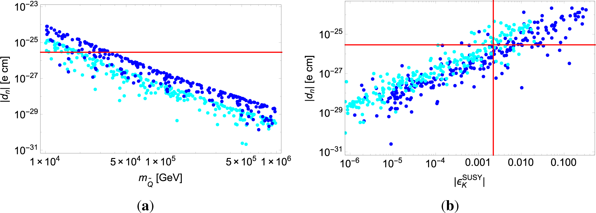
The nEDM and HgEDM are also sensitive to the SUSY contribution [61,70]. The gluino-squark interaction leads to the cEDM of quarks, which give the nEDM as shown in Equations (19) and (20). We show the predicted nEDM versus$m_{\tilde{Q}}$ for the case of the QCD sum rules of Equation (19) in Figure 3a, where the upper bound of |d_n| is shown by the red line. The plot is scattered due to the random phases of the squark mixing, as well as in the case of ϵ_K. We find that the contributions of EDM, d_d and d_u occupy around 25% of the neutron EDM. The SUSY contribution is close to the experimental upper bound up to 50 TeV. Since the predicted nEDM depends on the phases of the squark mixing matrix significantly, we plot the nEDM versus$|{ϵ}_K^{\text{SUSY}}|$ in Figure 3b. It is found that the predicted nEDM is roughly proportional to $|{ϵ}_K^{\text{SUSY}}|$. If the SUSY contribution is the level of $\mathcal{O}$ (10%) for ϵ_K, the nEDM is expected to be discovered in the region of 10⁻²⁷–10⁻²⁶ cm. On the other hand, if the nEDM is not observed above 10⁻²⁸ cm, the SUSY contribution of ϵ_K is below a few %. Thus, there is the correlation between d_n and ${ϵ}_K^{\text{SUSY}}$.

We also show the predicted HgEDM versus$m_{\tilde{Q}}$ for the case of the QCD sum rules of Equation (22) in Figure 4a, where the upper bound of $|d_{H_g}|$ is shown by the red line. The SUSY contribution is close to the experimental upper bound up to 200 TeV, which is much higher than the one of the nEDM. In Figure 4b, we plot the HgEDM versus$|{ϵ}_K^{\text{SUSY}}|$. It is found that the experimental upper bound of the HgEDM excludes completely $|{ϵ}_K^{\text{SUSY}}|$, which is inconsistent with the experimental data. If the SUSY contribution is the level of $\mathcal{O}$ (10%) for ϵ_K, the nEDM is expected to be discovered in the region of 10⁻²⁷–10⁻²⁶ cm. If the HgEDM is not observed above 10⁻²⁹ cm, the SUSY contribution of ϵ_K is below a few %. Thus, the mercury EDM gives more significant information for the gluino-squark interaction compared with the neutron EDM.

However, these correlations strongly depend on the assumptions of ${\theta }_{23}^L={\theta }_{13}^L$ and ${\theta }_{ij}^L={\theta }_{ij}^R$. The deviation from these relations destroys these correlations. For instance, for the case of ${\theta }_{23}^L\gg {\theta }_{13}^L$ with ${\theta }_{ij}^L={\theta }_{ij}^R$, ${ϵ}_K^{\text{SUSY}}$ is much suppressed, whereas the nEDM and HgEDM are still sizable. On the other hand, if ${\theta }_{ij}^L\gg {\theta }_{ij}^R$ or ${\theta }_{ij}^L\gg {\theta }_{ij}^R$ is realized, the cEDMs are suppressed, because they require the chirality flipping. In conclusion, careful studies of the mixing angle relations are required to test the correlations between EDMs and ${ϵ}_K^{\text{SUSY}}$.

We should comment on the hadronic model dependence of our numerical result. For both nEDM and HgEDM, we show the numerical result by using the hadronic model of the QCD sum rules in Equations (19) and (22). We have also calculated the EDMs by using the hadronic model of the chiral perturbation theory in Equations (20) and (23). For the neutron EDM, the prediction of the chiral perturbation theory is larger than the one of the QCD sum rule at most of a factor of two. However, for the mercury EDM, the prediction of the QCD sum rule is more than three-times larger compared with the one of the chiral perturbation theory. Thus, predicted EDMs have ambiguity with a factor of 2–3 from the hadronic model.

4.4. $D-\overline{D}$ Mixing

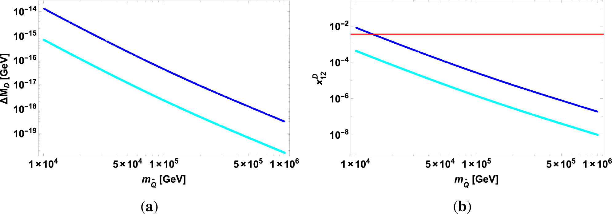
Since the SM prediction of ΔM_D at the short distance is $\mathcal{O}$ (10⁻¹⁸) GeV, which is very small compared with the experimental value due to the bottom quark loop, it is important to estimate the SUSY contribution of ΔM_D. The mixing angle ${\theta }_{ij}^{L(R)}$${\theta }_{ij}^{L(R)}$ also appears in the up-type squark mixing matrix, whereas the down-type squark mixing matrix contributes to the K⁰, B⁰ and B_s meson systems induced by the gluino-squark-quark interaction.

We show the SUSY component of ΔM_D and x_D versus$m_{\tilde{Q}}$ for s₁₃ = s₂₃ = 0.22, 0.5 in Figure 5. At the SUSY scale of 10 TeV, the SUSY component may be comparable to the observed value. Although the accurate estimate of the long-distance effect is difficult, Cheng and Chiang estimated x_D of order 10⁻³ from the two body hadronic modes [85]. This obtained value is consistent with the experimental one. Therefore, we should take into account the long-distance effect properly in order to constrain the SUSY contribution from ΔM_D.

Before closing the presentation of the numerical results, we add a comment on the other gaugino contribution. There are additional contributions to the FCNC induced by chargino exchanging diagrams. The chargino contribution to the gluino one is approximately 10% in the above numerical study of ΔF = 2. Thus, the chargino contributions are the sub-leading ones.

5. Summary

We discussed the sensitivity of the high-scale SUSY at 10–1000 TeV in the B⁰, B_s and K⁰ meson systems. Furthermore, we have also discussed the sensitivity to the $D-\overline{D}$ mixing, the neutron EDM and the mercury EDM. In order to estimate the contribution of the squark flavor mixing to these FCNC, we calculate the squark mass spectrum, which is consistent with the recent Higgs discovery.

The SUSY contributions in $\mathrm{\Delta }{M}_{B_s}$ and ΔM_Bs are at most 1.5% and 0.1% at $m_{\tilde{Q}}=10\text{TeV}$, respectively. As $m_{\tilde{Q}}$ increases, the SUSY contributions of both $\mathrm{\Delta }{M}_{B^0}$ and $\mathrm{\Delta }{M}_{B_s}$ decrease approximately with the power of $1/m_{\tilde{Q}}^2$. Therefore, the SUSY scale increases to more than 10 TeV, and no signal of SUSY is expected. On the other hand, the SUSY contribution in $M_{K^0}$ can be comparable to the experimental value in the case of s₁₃ = s₂₃ = 0.5, whereas it is suppressed in the case of s₁₃ = s₂₃ = 0.22 at $m_{\tilde{Q}}=10\text{TeV}$. Furthermore, the SUSY contribution in ϵ_K could be large, around 40% in the region of the SUSY scale 10–100 TeV. By considering the effect of the SUSY contribution O(10%) in ϵ_K, the tension between ϵ_K and sin φ_d can be relaxed even if the SUSY scale is 100 TeV.

The neutron EDM and the mercury EDM are also sensitive to the SUSY contribution induced by the gluino-squark interaction. The |d_n| is expected to be close to the experimental upper bound, even if the SUSY scale is 50 TeV. The predicted nEDM is roughly proportional to $|{ϵ}_K^{\text{SUSY}}|$. If the SUSY contribution is the level of $\mathcal{O}$ (10%) for ϵ_K, the |d_n| is expected to be discovered in the region of 10⁻²⁷−10⁻²⁶ cm. For the |d_Hg|, the SUSY contribution is close to the experimental upper bound up to 200TeV, which is much higher than the one of the nEDM. If the HgEDM is not observed above 10⁻²⁹ cm, the SUSY contribution of ϵ_K is below a few %. Thus, the mercury EDM gives more significant information for the gluino-squark interaction compared with the neutron EDM. It may be important to give a comment that these predictions depend strongly on the assumptions of ${\theta }_{23}^L={\theta }_{13}^L$ and ${\theta }_{ij}^L={\theta }_{ij}^R$. The deviation from these relations destroys these correlations. In conclusion, careful studies of the mixing angle relations are required to test the correlations between EDMs and ${ϵ}_K^{\text{SUSY}}$. The predicted EDMs have also ambiguity with the factor of 2–3 from the hadronic model.

Since the SM prediction of ΔM_D at the short distance is $\mathcal{O}$ (10⁻¹⁸) GeV, which is very small compared with the experimental value, it is important to estimate the SUSY contribution of ΔM_D.

In conclusion, more detailed studies of the K⁰ meson system, the EDMs of the neutron and mercury are required in order to probe the high-scale SUSY at 10–1000 TeV.

References

- Aad, G.; Abbott, B.; Abdallah, J.; Abdel Khalek, S.; Abdinov, O.; Aben, R.; Abi, B.; Abolins, M.; AbouZeid, O.S.; Abramowicz, H.; et al. Search for squarks and gluinos with the ATLAS detector in final states with jets and missing transverse momentum using TeV proton–proton collision data. J. High Energy Phys. 2014, 176, 1–52. [Google Scholar]
- Chatrchyan, S.; Khachatryan, V.; Sirunyan, A.M.; Tumasyan, A.; Adam, W.; Bergauer, T.; Dragicevic, M.; Ero, J.; Fabjan, C.; Friedl, M.; et al. Search for new physics in the multijet and missing transverse momentum final state in proton-proton collisions at TeV. J. High Energy Phys. 2014, 055. [Google Scholar] [CrossRef]
- Aad, G.; Abbott, B.; Abdallah, J.; Abdel Khalek, S.; Abdinov, O.; Aben, R.; Abi, B.; Abolins, M.; AbouZeid, O.S.; Abramowicz, H.; et al. Search for top squark pair production in final states with one isolated lepton, jets, and missing transverse momentum in TeV pp collisions with the ATLAS detector. J. High Energy Phys. 2014, 118. [Google Scholar] [CrossRef]
- Aad, G.; Abbott, B.; Abdallah, J.; Abdel Khalek, S.; Abdinov, O.; Aben, R.; Abi, B.; Abolins, M.; AbouZeid, O.S.; Abramowicz, H.; et al. Observation of a new particle in the search for the Standard Model Higgs boson with the ATLAS detector at the LHC. Phys. Lett. B. 2012, 716, 1–29. [Google Scholar]
- Chatrchyan, S.; Khachatryan, V.; Sirunyan, A.M.; Tumasyan, A.; Adam, W.; Bergauer, T.; Dragicevic, M.; Ero, J.; Fabjan, C.; Friedl, M.; et al. Observation of a new boson at a mass of 125 GeV with the CMS experiment at the LHC. Phys. Lett. B. 2012, 716, 30–61. [Google Scholar]
- Aad, G.; Abbott, B.; Abdallah, J.; Abdel Khalek, S.; Abdinov, O.; Aben, R.; Abi, B.; Abolins, M.; AbouZeid, O.S.; Abramowicz, H.; et al. Combined Measurement of the Higgs Boson Mass in pp Collisions at and 8 TeV with the ATLAS and CMS Experiments. 2015. arXiv:1503.07589. arXiv.org e-Print archive. Available online: http://arxiv.org/abs/1503.07589 accessed on 14 May 2015. [Google Scholar]
- Giudice, G.F.; Luty, M.A.; Murayama, H.; Rattazzi, R. Gaugino mass without singlets. J. High Energy Phys. 1998, 027. [Google Scholar] [CrossRef]
- Wells, J.D. Implications of supersymmetry breaking with a little hierarchy between gauginos and scalars, 2003. arXiv:hep-ph/0306127. arXiv.org e-Print archive Available online: http://arxiv.org/abs/hep-ph/0306127 accessed on 14 May 2015.
- Arkani-Hamed, N.; Dimopoulos, S. Supersymmetric unification without low energy supersymmetry and signatures for fine-tuning at the LHC, 2004. arXiv:hep-th/0405159. arXiv.org e-Print archive Available online: http://arxiv.org/abs/hep-th/0405159 accessed on 14 May 2015.
- Giudice, G.F.; Romanino, A. Split supersymmetry. Nucl. Phys. B. 2004, 699, 65–89. [Google Scholar]
- Arkani-Hamed, N.; Dimopoulos, S.; Giudice, G.F.; Romanino, A. Aspects of split supersymmetry. Nucl. Phys. B. 2005, 709, 3–46. [Google Scholar]
- Wells, J.D. PeV-scale supersymmetry. Phys. Rev. D. 2005, 71. [Google Scholar] [CrossRef]
- Ibe, M.; Moroi, T.; Yanagida, T.T. Possible Signals of Wino LSP at the Large Hadron Collider. Phys. Lett. B. 2007, 644, 355–360. [Google Scholar]
- Hall, L.J.; Nomura, Y. A Finely-Predicted Higgs Boson Mass from A Finely-Tuned Weak Scale. J. High Energy Phys. 2010, 076. [Google Scholar] [CrossRef]
- Hall, L.J.; Nomura, Y. Spread Supersymmetry. J. High Energy Phys. 2012, 082. [Google Scholar] [CrossRef]
- Ibe, M.; Yanagida, T.T. The Lightest Higgs Boson Mass in Pure Gravity Mediation Model. Phys. Lett. B. 2012, 374, 374–380. [Google Scholar]
- Ibe, M.; Matsumoto, S.; Yanagida, T.T. Pure Gravity Mediation with m3/2 = 10–100 TeV. Phys. Rev. D. 2012, 85. [Google Scholar] [CrossRef]
- Arvanitaki, A.; Craig, N.; Dimopoulos, S.; Villadoro, G. Mini-Split. J. High Energy Phys. 2013, 126. [Google Scholar] [CrossRef]
- Arkani-Hamed, N.; Gupta, A.; Kaplan, D.E.; Weiner, N.; Zorawski, T. Simply Unnatural Supersymmetry, 2012. arXiv:1212.6971. arXiv.org e-Print archive Available online: http://arxiv.org/abs/1212.6971 accessed on 14 May 2015.
- Evans, J.L.; Ibe, M.; Olive, K.A.; Yanagida, T.T. Universality in Pure Gravity Mediation. Eur. Phys. J. C. 2013, 73. [Google Scholar] [CrossRef]
- Hisano, J.; Kuwahara, T.; Nagata, N. Grand Unification in High-scale Supersymmetry. Phys. Lett. B. 2013, 723, 324–329. [Google Scholar]
- Nagata, N.; Otono, H.; Shirai, S. Probing Bino-Gluino Coannihilation at LHC, 2015. arXiv:1504.00504. arXiv.org e-Print archive Available online: http://arxiv.org/abs/1504.00504 accessed on 14 May 2015.
- Altmannshofer, W.; Harnik, R.; Zupan, J. Low Energy Probes of PeV Scale Sfermions. J. High Energy Phys. 2013, 202. [Google Scholar] [CrossRef]
- Moroi, T.; Nagai, M. Probing Supersymmetric Model with Heavy Sfermions Using Leptonic Flavor and CP Violations. Phys. Lett. B. 2013, 723, 107–112. [Google Scholar]
- McKeen, D.; Pospelov, M.; Ritz, A. Electric dipole moment signatures of PeV-scale superpartners. Phys. Rev. D. 2013, 87. [Google Scholar] [CrossRef]
- Aaij, R.; Beteta, C.A.; Adeva, B.; Adinolfi, M.; Adrover, C.; Affolder, A.; Ajaltouni, Z.; Albrecht, J.; Alessio, F.; Alexander, M.; et al. Implications of LHCb measurements and future prospects. Eur. Phys. J. C. 2013, 73, 1–92. [Google Scholar]
- Aaij, R.; Beteta, C.A.; Adeva, B.; Adinolfi, M.; Adrover, C.; Affolder, A.; Ajaltouni, Z.; Albrecht, J.; Alessio, F.; Alexander, M.; et al. First measurement of the CP-violating phase in decays. 2013. arXiv:1303.7125. arXiv.org e-Print archive. Available online: http://arxiv.org/abs/1303.7125 accessed on 14 May 2015. [Google Scholar]
- Aaij, R.; Beteta, C.A.; Adeva, B.; Adinolfi, M.; Adrover, C.; Affolder, A.; Ajaltouni, Z.; Albrecht, J.; Alessio, F.; Alexander, M.; et al. First observation of CP violation in the decays of mesons. 2013. arXiv:1304.6173. arXiv.org e-Print archive. Available online: http://arxiv.org/abs/1304.6173 accessed on 14 May 2015. [Google Scholar]
- Aaij, R.; Beteta, C.A.; Adeva, B.; Adinolfi, M.; Adrover, C.; Affolder, A.; Ajaltouni, Z.; Albrecht, J.; Alessio, F.; Alexander, M.; et al. Measurement of CP violation and the meson decay width difference with and decays. 2013. arXiv:1304.2600. arXiv.org e-Print archive. Available online: http://arxiv.org/abs/1304.2600 accessed on 14 May 2015. [Google Scholar]
- Aaij, R.; Beteta, C.A.; Adeva, B.; Adinolfi, M.; Adrover, C.; Affolder, A.; Ajaltouni, Z.; Albrecht, J.; Alessio, F.; Alexander, M.; et al. Differential branching fraction and angular analysis of the decay . J. High Energy Phys. 2013. [Google Scholar] [CrossRef]
- Aaij, R.; Beteta, C.A.; Adeva, B.; Adinolfi, M.; Adrover, C.; Affolder, A.; Ajaltouni, Z.; Albrecht, J.; Alessio, F.; Alexander, M.; et al. Differential branching fraction and angular analysis of the decay B0 → K∗0µ+µ−, 2013. arXiv:1304.6325. arXiv.org e-Print archive. Available online: http://arxiv.org/abs/1304.6325 accessed on 14 May 2015.
- Aaij, R.; Beteta, C.A.; Adeva, B.; Adinolfi, M.; Adrover, C.; Affolder, A.; Ajaltouni, Z.; Albrecht, J.; Alessio, F.; Alexander, M.; et al. Precision measurement of the oscillation frequency with the decay . 2013. arXiv:1304.4741. arXiv.org e-Print archive. Available online: http://arxiv.org/abs/1304.4741 accessed on 14 May 2015. [Google Scholar]
- Vesterinen, M. LHCb Semileptonic Asymmetry, 2013. arXiv:1306.0092. arXiv.org e-Print archive Available online: http://arxiv.org/abs/1306.0092 accessed on 14 May 2015.
- Aaij, R.; Beteta, C.A.; Adeva, B.; Adinolfi, M.; Adrover, C.; Affolder, A.; Ajaltouni, Z.; Albrecht, J.; Alessio, F.; Alexander, M.; et al. First evidence for the decay B− → K∗0µ+µ−, 2012. arXiv:1211.2674. arXiv.org e-Print archive. Available online: http://arxiv.org/abs/1211.2674 accessed on 14 May 2015.
- Aaij, R.; Beteta, C.A.; Adeva, B.; Adinolfi, M.; Adrover, C.; Affolder, A.; Ajaltouni, Z.; Albrecht, J.; Alessio, F.; Alexander, M.; et al. Measurement of the CP asymmetry in B0 → K∗0µ+µ− decays, 2012. arXiv:1210.4492. arXiv.org e-Print archive. Available online: http://arxiv.org/abs/1210.4492 accessed on 14 May 2015.
- Amhis, Y.; Banerjee, Sw.; Bernhard, R.; Blyth, S.; Bozek, A.; Bozzi, C.; Carbone, A.; Campos, A.O.; Chistov, R.; Cibinetto, G.; et al. Averages of B-hadron, C-hadron, and tau-lepton properties as of early 2012, 2012. arXiv:1207.1158. arXiv.org e-Print archive. Available online: http://arxiv.org/abs/1207.1158 accessed on 14 May 2015.
- Aaij, R.; Beteta, C.A.; Adeva, B.; Adinolfi, M.; Adrover, C.; Affolder, A.; Ajaltouni, Z.; Albrecht, J.; Alessio, F.; Alexander, M.; et al. Measurement of the CP-violating phase ϕs in the decay . 2011. arXiv:1112.3183. arXiv.org e-Print archive. Available online: http://arxiv.org/abs/1112.3183 accessed on 14 May 2015. [Google Scholar]
- Aaij, R.; Beteta, C.A.; Adeva, B.; Adinolfi, M.; Adrover, C.; Affolder, A.; Ajaltouni, Z.; Albrecht, J.; Alessio, F.; Alexander, M.; et al. Measurement of the CP violating phase ϕs in . 2011. arXiv:1112.3056.arXiv.org e-Print archive. Available online: http://arxiv.org/abs/1112.3056 accessed on 14 May 2015. [Google Scholar]
- Kobayashi, M.; Maskawa, T. CP Violation in the Renormalizable Theory of Weak Interaction. Prog. Theor. Phys. 1973, 49, 652–657. [Google Scholar]
- Gabbiani, F.; Gabrielli, E.; Masiero, A.; Silvestrini, L. A Complete analysis of FCNC and CP constraints in general SUSY extensions of the standard model. Nucl. Phys. B. 1996, 477, 321–352. [Google Scholar]
- Tanimoto, M.; Yamamoto, K. Probing the high scale SUSY in CP violations of K, B0 and Bs mesons, 2014. arXiv:1404.0520. arXiv.org e-Print archive. Available online: http://arxiv.org/abs/1404.0520 accessed on 14 May 2015.
- Charles, J.; Descotes-Genon, S.; Ligeti, Z.; Monteil, S.; Papucci, M.; Trabelsi, K. Future sensitivity to new physics in Bd, Bs, and K mixings. Phys. Rev. D. 2014, 89. [Google Scholar] [CrossRef]
- King, S.F. Implications of large CP Violation in B mixing for Supersymmetric Standard Models. J. High Energy Phys. 2010, 114. [Google Scholar] [CrossRef]
- Endo, M.; Shirai, S.; Yanagida, T.T. Split Generation in the SUSY Mass Spectrum and Mixing. Prog. Theor. Phys. 2011, 125, 921–932. [Google Scholar]
- Endo, M.; Yokozaki, N. Large CP Violation in Bs Meson Mixing with EDM constraint in Supersymmetry. J. High Energy Phys. 2011, 130. [Google Scholar] [CrossRef]
- Kubo, J.; Lenz, A. Large loop effects of extra SUSY Higgs doublets to CP violation in B0 mixing. Phys. Rev. D. 2010, 82. [Google Scholar] [CrossRef]
- Kaburaki, Y.; Konya, K.; Kubo, J.; Lenz, A. Triangle Relation of Dark Matter, EDM and CP Violation in B0 Mixing in a Supersymmetric Q6 Model, 2010. arXiv:1012.2435. arXiv.org e-Print archive Available online: http://arxiv.org/abs/1012.2435 accessed on 14 May 2015.
- Virto, J. Exact NLO strong interaction corrections to the Delta F = 2 effective Hamiltonian in the MSSM, 2009. arXiv:0907.5376. arXiv.org e-Print archive. Available online: http://arxiv.org/abs/0907.5376 accessed on 14 May 2015.
- Virto, J. Top mass dependent corrections to B-meson mixing in the MSSM. 2011. arXiv:1111.0940. arXiv.org e-Print archive Available online: http://arxiv.org/abs/1111.0940 accessed on 14 May 2015. [Google Scholar]
- Ko, P.; Park, J.-H. Implications of the measurements of mixing on SUSY models. 2008. arXiv:0809.0705. arXiv.org e-Print archive Available online: http://arxiv.org/abs/0809.0705 accessed on 14 May 2015. [Google Scholar]
- Ko, P.; Park, J.-H. Addendum to: Implications of the measurements of bar mixing on SUSY models. 2010. arXiv:1006.5821. arXiv.org e-Print archive. Available online: http://arxiv.org/abs/1006.5821 accessed on 14 May 2015. [Google Scholar]
- Wang, R.M.; Xu, Y.G.; Chang, Q.; Yang, Y.D. Studying of mixing and Bs → K(∗)−K(∗)+ decays within supersymmetry. Phys. Rev. D. 2011, 83. [Google Scholar] [CrossRef]
- Parry, J.K. The Like-sign dimuon charge asymmetry in SUSY models, 2010. arXiv:1006.5331. arXiv.org e-Print archive Available online: http://arxiv.org/abs/1006.5331 accessed on 14 May 2015.
- Hayakawa, A.; Shimizu, Y.; Tanimoto, M.; Yamamoto, K. Squark flavor mixing and CP asymmetry of neutral B mesons at LHCb. Nucl. Phys. B. 2012, 710, 446–453. [Google Scholar]
- Shimizu, Y.; Tanimoto, M.; Yamamoto, K. Direct CP Violation of b → sγ and CP Asymmetries of Non-Leptonic B Decays in Squark Flavor Mixing, 2012. arXiv:1205.1705. arXiv.org e-Print archive Available online: http://arxiv.org/abs/1205.1705 accessed on 14 May 2015.
- Shimizu, Y.; Tanimoto, M.; Yamamoto, K. SUSY contributions to CP violations in b → s and b → d transitions facing on new data, 2012. arXiv:1212.6486. arXiv.org e-Print archive. Available online: http://arxiv.org/abs/1212.6486 accessed on 14 May 2015.
- Shimizu, Y.; Tanimoto, M.; Yamamoto, K. Sensitivity of the squark flavor mixing to the CP violation of K, B0 and Bs mesons, 2013. arXiv:1307.0374. arXiv.org e-Print archive. Available online: http://arxiv.org/abs/1307.0374 accessed on 14 May 2015.
- Hayakawa, A.; Shimizu, Y.; Tanimoto, M.; Yamamoto, K. Searching for the squark flavor mixing in CP violations of and K0K−0 decays. 2013. arXiv:1311.5974. arXiv.org e-Print archive. Available online: http://arxiv.org/abs/1311.5974 accessed on 14 May 2015. [Google Scholar]
- Mescia, F.; Virto, J. Natural SUSY and Kaon Mixing in view of recent results from Lattice QCD, 2012. arXiv:1208.0534. arXiv.org e-Print archive Available online: http://arxiv.org/abs/1208.0534 accessed on 14 May 2015.
- Tanimoto, M.; Yamamoto, K. decay correlating with ϵK in high-scale SUSY. 2015. arXiv:1503.06270. arXiv.org e-Print archive. Available online: http://arxiv.org/abs/1503.06270 accessed on 14 May 2015. [Google Scholar]
- Fuyuto, K.; Hisano, J.; Nagata, N.; Tsumura, K. QCD Corrections to Quark (Chromo)Electric Dipole Moments in High-scale Supersymmetry, 2013. arXiv:1308.6493. arXiv.org e-Print archive Available online: http://arxiv.org/abs/1308.6493 accessed on 14 May 2015.
- Olive, K.A.; Agashe, K.; Amsler, C.; Antonelli, M.; Arguin, J.-F.; Asner, D.M.; Baer, H.; Band, H.R.; Barnett, R.M.; Basaglia, T.; et al. Review of Particle Physics. Chin. Phys. C. 2014, 38. [Google Scholar] [CrossRef]
- Pospelov, M.; Ritz, A. Neutron EDM from electric and chromoelectric dipole moments of quarks. Phys. Rev. D. 2001, 63. [Google Scholar] [CrossRef]
- Hisano, J.; Shimizu, Y. B → ϕKs versus electric dipole moment of Hg-199 atom in supersymmetric models with right-handed squark mixing. Phys. Lett. B. 2004, 581, 224–230. [Google Scholar]
- Hisano, J.; Shimizu, Y. Hadronic electric dipole moments induced by the strangeness and constraints on supersymmetric CP phases. Phys. Rev. D. 2004, 70, 093001. [Google Scholar] [CrossRef]
- Hisano, J.; Nagai, M.; Paradisi, P. Flavor effects on the electric dipole moments in supersymmetric theories: A beyond leading order analysis. Phys. Rev. D. 2009, 80, 095014. [Google Scholar] [CrossRef]
- Hisano, J.; Lee, J.Y.; Nagata, N.; Shimizu, Y. Reevaluation of Neutron Electric Dipole Moment with QCD Sum Rules. Phys. Rev. D. 2012, 85. [Google Scholar] [CrossRef]
- Fuyuto, K.; Hisano, J.; Nagata, N. Neutron Electric Dipole Moment Induced by the Strangeness Revisited, 2012. arXiv:1211.5228. arXiv.org e-Print archive Available online: http://arxiv.org/abs/1211.5228 accessed on 14 May 2015.
- Griffith, W.C.; Swallows, M.D.; Loftus, T.H.; Romalis, M.V.; Heckel, B.R.; Fortson, E.N. Improved Limit on the Permanent Electric Dipole Moment of Hg-199. Phys. Rev. Lett. 2009, 102, 101601. [Google Scholar] [CrossRef]
- Chiou, C.C.; Kong, O.C.; Vaidya, R.D. Quark Loop Contributions to Neutron, Deuteron, and Mercury EDMs from Supersymmetry without R parity, 2007. arXiv:0705.3939. arXiv.org e-Print archive Available online: http://arxiv.org/abs/0705.3939 accessed on 14 May 2015.
- Delgado, A.; Garcia, M.; Quiros, M. Electroweak and supersymmetry breaking from the Higgs boson discovery, 2013. arXiv:1312.3235. arXiv.org e-Print archive Available online: http://arxiv.org/abs/1312.3235 accessed on 14 May 2015.
- Giudice, G.F.; Rattazzi, R. Living Dangerously with Low-Energy Supersymmetry. Nucl. Phys. B. 2006, 757, 19–46. [Google Scholar]
- Martin, S.P. A Supersymmetry primer, 2011. arXiv:9709356. arXiv.org e-Print archive Available online: http://arxiv.org/pdf/hep-ph/9709356 accessed on 14 May 2015.
- Iso, S. What Can We Learn from the 126 GeV Higgs Boson for the Planck Scale Physics? -Hierarchy Problem and the Stability of the Vacuum-, 2013. arXiv:1304.0293. arXiv.org e-Print archive Available online: http://arxiv.org/abs/1304.0293 accessed on 14 May 2015.
- Iso, S.; Orikasa, Y. TeV Scale B-L model with a flat Higgs potential at the Planck scale—In view of the hierarchy problem, 2012. arXiv:1210.2848. arXiv.org e-Print archive Available online: http://arxiv.org/abs/1210.2848 accessed on 14 May 2015.
- Bian, L.G. RGE of the Higgs mass in the context of the SM, 2013. arXiv:1303.2402. arXiv.org e-Print archive Available online: http://arxiv.org/abs/1303.2402 accessed on 14 May 2015.
- Buras, A.J.; Guadagnoli, D. Correlations among new CP violating effects in ΔF = 2 observables, 2008. arXiv:0805.3887. arXiv.org e-Print archive. Available online: http://arxiv.org/abs/0805.3887 accessed on 14 May 2015.
- Inami, T.; Lim, C.S. Effects of Superheavy Quarks and Leptons in Low-Energy Weak Processes KL → µµ−, K+ → π+vv− and K0 ↔ K−0. Prog. Theor. Phys. 1981, 65, 297–314. [Google Scholar]
- Bae, T.; Jang, Y.C.; Jeong, H.; Kim, J.; Kim, J.; Kim, K.; Kim, S.; Lee, W.; Leem, J.; Pak, J.; et al. Update on BK and εK with staggered quarks. 2013. arXiv:1310.7319. arXiv.org e-Print archive. Available online: http://arxiv.org/abs/1310.7319 accessed on 14 May 2015. [Google Scholar]
- Aoki, S.; Aoki, Y.; Bernard, C.; Blum, T.; Colangelo, G.; Della Morte, M.; Durr, S.; Khadra, A.X.E.; Fukaya, H.; Horsley, R.; et al. Review of lattice results concerning low energy particle physics, 2013. arXiv:1310.8555. arXiv.org e-Print archive. Available online: http://arxiv.org/abs/1310.8555 accessed on 14 May 2015.
- Falk, T.; Olive, K.A.; Pospelov, M.; Roiban, R. MSSM predictions for the electric dipole moment of the Hg-199 atom. Nucl. Phys. B. 1999, 560, 3–22. [Google Scholar]
- Hisano, J.; Kakizaki, M.; Nagai, M.; Shimizu, Y. Hadronic EDMs in SUSY SU (5) GUTs with right-handed neutrinos. Phys. Lett. B. 2004, 604, 216–224. [Google Scholar]
- Bevan, A.J.; Bona, M.; Ciuchini, M.; Derkach, D.; Franco, E.; Lubicz, V.; Martinelli, G.; Parodi, F.; Pierini, M.; Schiavi, C.; Silvestrini, L.; et al. The UTfit collaboration average of D meson mixing data: Winter 2014. J. High Energy Phys. 2014, 123. [Google Scholar] [CrossRef]
- UTfit, Available online: http:/www.utfit.org accessed on 14 May 2015.
- Cheng, H.Y.; Chiang, C.W. Long-Distance Contributions to Mixing Parameters. 2010. arXiv:1005.1106. arXiv.org e-Print archive Available online: http://arxiv.org/abs/1005.1106 accessed on 14 May 2015. [Google Scholar]
- Toru Goto, Available online: http://research.kek.jp/people/tgoto/ accessed on 14 May 2015.
- Becirevic, D.; Gimenez, V.; Martinelli, G.; Papinutto, M.; Reyes, J. B parameters of the complete set of matrix elements of delta B = 2 operators from the lattice. J. High Energy Phys. 2002, 025. [Google Scholar] [CrossRef]
- Allton, C.R.; Conti, L.; Donini, A.; Gimenez, V.; Giusti, L.; Martinelli, G.; Talevi, M.; Vladikas, A. B parameters for Delta S = 2 supersymmetric operators. Phys. Lett. B. 1999, 453, 30–39. [Google Scholar]
- Buras, A.J.; Misiak, M.; Urban, J. Two loop QCD anomalous dimensions of flavor changing four quark operators within and beyond the standard model. Nucl. Phys. B. 2000, 586, 397–426. [Google Scholar]
- Carrasco, N.; Ciuchini, M.; Dimopoulos, P.; Frezzotti, R.; Gimenez, V.; Lubicz, V.; Rossi, G.C.; Sanfilippo, F.; Silvestrini, L.; Simula, S.; et al. mixing in the standard model and beyond from Nf = 2 twisted mass QCD. Phys. Rev. D. 2014, 90, 014502. [Google Scholar] [CrossRef]
- Degrassi, G.; Franco, E.; Marchetti, S.; Silvestrini, L. QCD corrections to the electric dipole moment of the neutron in the MSSM. J. High Energy Phys. 2005, 044. [Google Scholar] [CrossRef]
© 2015 by the authors; licensee MDPI, Basel, Switzerland This article is an open access article distributed under the terms and conditions of the Creative Commons Attribution license (http://creativecommons.org/licenses/by/4.0/).
Share and Cite
Tanimoto, M.; Yamamoto, K. Sensitivity of High-Scale SUSY in Low Energy Hadronic FCNC. Symmetry 2015, 7, 689-713. https://doi.org/10.3390/sym7020689
Tanimoto M, Yamamoto K. Sensitivity of High-Scale SUSY in Low Energy Hadronic FCNC. Symmetry. 2015; 7(2):689-713. https://doi.org/10.3390/sym7020689
Chicago/Turabian StyleTanimoto, Morimitsu, and Kei Yamamoto. 2015. "Sensitivity of High-Scale SUSY in Low Energy Hadronic FCNC" Symmetry 7, no. 2: 689-713. https://doi.org/10.3390/sym7020689