Analysis of Ilmenite Slag Using Laser-Induced Breakdown Spectroscopy

Abstract

The feasibility of using laser-induced breakdown spectroscopy (LIBS) for the compositional analysis of ilmenite slag was explored. The slag was obtained from a pilot-scale ilmenite smelting furnace. The composition of major oxides TiO₂, FeO, and MgO are determined by the calibrated LIBS method. LIBS measurements are done under normal atmosphere and temperature. A Q-switched Nd:YAG laser operating at 355 nm was used to create a plasma on an ilmenite slag sample. The characteristic lines based on the NIST database of Fe, Mg, and Ti can be identified on the normalized LIBS spectra for the slag samples. The spectral range chosen for the study is 370 to 390 nm. Calibration curves were plotted using the data collected from various industrial ilmenite samples of varying compositions of TiO₂, FeO, and MgO. The univariate simple linear regression technique was used to do the analysis and the prediction accuracy was checked by the root mean square error (RMSE). To validate the application of LIBS, both qualitative and quantitative analysis is done and compared to the analytical ICP-OES results. The model predicts the magnesium content with the highest accuracy and gives good prediction for iron and titanium content. This study demonstrates the capability of using LIBS for the surface analysis of the ilmenite slag sample.

1. Introduction

Ilmenite smelting is a reduction process in which the FeO in ilmenite is reduced to Fe, giving a titanium-rich slag on top of pure pig iron [1]. Slags analysis is of great importance in ilmenite smelting as the slag contains the titanium oxide and the pure pig iron is the by-product [2,3]. The slag composition is checked during the process to see the titania content. Ideally, a measurement technique should be able to perform measurements inside the furnace, giving slag conditions in a very short period. However, due to technical difficulties, this requirement is fulfilled by taking out a small amount of sample from the furnace and letting it cool, which is later sent to the laboratory, where suitable techniques (such as X-ray fluorescence) are used to analyze the slag for its composition. This consumes time, and during the test period the furnace consumes energy and feed material. Any reduction in the analysis time will impact the quality and productivity of the smelting process and it can be achieved by an online measurement technique or by analyzing the slag at a higher temperature. We are exploring the possibility to use laser-induced breakdown spectroscopy (LIBS) as an analytical technique to do an in-situ analysis of the slag. A successful analysis of samples at room temperature will pave the way for higher temperature ilmenite slag analysis using LIBS.

The advantage of using LIBS over other surface techniques is the ability to carry out the measurement by maintaining a distance from the plasma, which is formed by laser radiation. Other advantages include fast measurement time, no sample preparation and most of the elements can be analyzed such as solid bulk samples, liquid, gases, and micro and nanoparticles [4]. These advantages make LIBS an ideal method for online monitoring of the slag condition. However, it has to be tested for its accuracy and usability in practical conditions. One disadvantage of using LIBS is that it gives information only about the surface of the sample with depth penetration of one to two millimeters [5].

Multi-component oxide materials have been measured quantitatively using LIBS such as steel at high temperatures, metallurgical slags, concrete, rocks, and ceramics [6,7]. Oxide inclusion in steel products has been investigated before using LIBS [8]. One of the earliest in-situ analyses using LIBS was done for surface analyses of elemental concentration in various liquid and solid samples in 1992 [9]. Many real-time monitoring applications using LIBS are in use for the iron and steel making processes [10,11]. For the quantitative analysis of materials, two methods are available. The most common method is to use a calibration-based method where a calibration curve is plotted using reference samples. Methods such as a support vector mechanism and partial least square have been used to perform quantitative analysis of various slag samples [12]. The other method is a calibration-free method where the composition is measured directly from the LIBS spectra by modeling the optical plasma emission [13]. Even though LIBS has been used in the research of both solid and liquid slag samples, the majority of the samples are from steel slags [14,15].

In the case of ilmenite smelting, the slag analysis becomes very important as the slag composition changes rapidly with process condition and any delay in slag analysis can alter the slag composition in the furnace. In this paper, we report about the investigation of multi-component oxides by LIBS and the quantitative analysis of major oxides in ilmenite slag by a calibration-based method. The oxide materials are ilmenite slag samples from industry and the investigated components are TiO₂, FeO, and MgO. Other impurities such as SiO₂, MnO, and Al₂O₃ are not considered for this study as they are not present in high quantity and do not play an important role in the process condition of ilmenite smelting or slag formation. The concentration of FeO and MgO in the ilmenite slag is important as FeO can be related to foaming issues and correlates with the amount of Ti₂O₃ formed whereas low MgO is required for the chlorination process to get TiO₂ pigment. Industrial slags normally consist of impurities amounting to around 3% of SiO₂, MnO, and Al₂O₃ [1]. The concentration of the impurities depends on the ilmenite mineral feed. A laboratory-based LIBS setup is used for experiments on various slag samples.

2. Materials and Methods

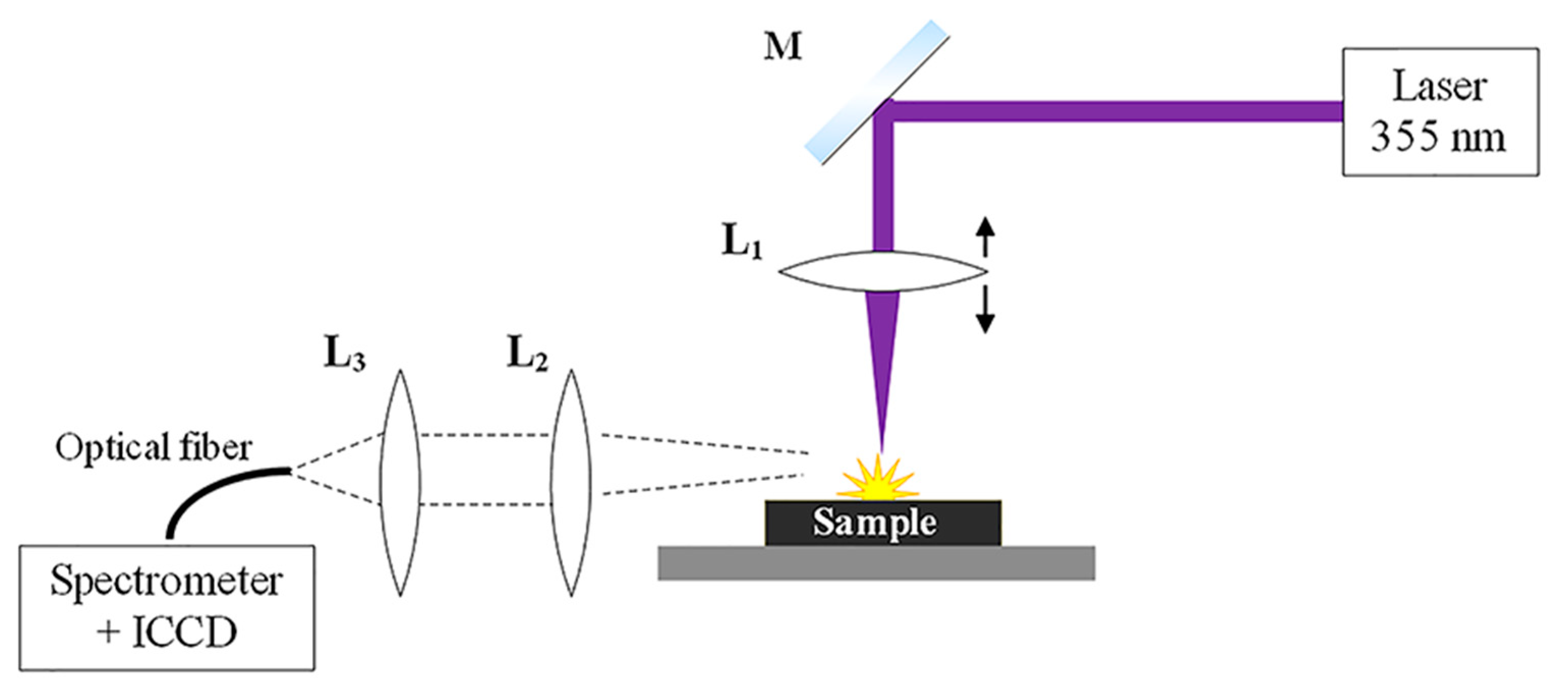
2.1. LIBS Setup

A schematic diagram of the experimental set-up used for the study is shown in Figure 1. A laser pulse of 355 nm with a pulse energy of around 6 mJ and a pulse duration of around 5 ns at a frequency of 10 Hz was used for laser ablation. As seen in Figure 1, the laser pulse beam was reflected using mirror M (aluminum UV-enhanced mirrors, reflection > 99.5%) with a motive to direct the pulses on the top surface of the sample. Pulses were focused onto the sample surface by a fused silica plano-convex lens L₁ of 50 mm focal length.

The lens is mounted on a translation stage (15 mm range) which allows fine adjustment of the focal point. To maximize and stabilize plasma formation and emission, the intensity of the focal point was decided to shift at 400 microns below the sample surface. This also limits the risk of a breakdown in the atmosphere in case of fluctuations of the sample surface. The value of 400 microns has been set after optimization in relation to the nature of the sample [16,17]. The ablation from the surface occurred in an ambient atmosphere and the light emitted from the plasma was collected along an axis perpendicular to the incident pulse by a plano-convex lens L₂ of 75 mm focal length. The collimated light was then focused onto a round-to-linear bundle of 7 × 200 µm core multimode fibers (resulting in a higher coupling efficiency into the spectrometer) by another plano-convex lens L₃ with a 50 mm focal length and directed to the spectrometer coupled to an ICCD camera. A Czerny-Turner spectrometer (Kymera, Andor Technology, Abingdon, Oxfordshire, UK) was used with a 2400 lines/mm grating which had a spectral resolution of 0.2 nm for a spectral range of 25 nm. The output from the spectrometer was directed to an ICCD camera (iStar Andor technology, Abingdon, Oxfordshire, UK). The ICCD camera was synchronized to the laser pulse by a trigger signal from the laser. The acquisition of the spectrum was conducted using delay and gate width of respectively, 500 and 2000 ns after the laser pulse. Those values were optimized for this setup configuration.

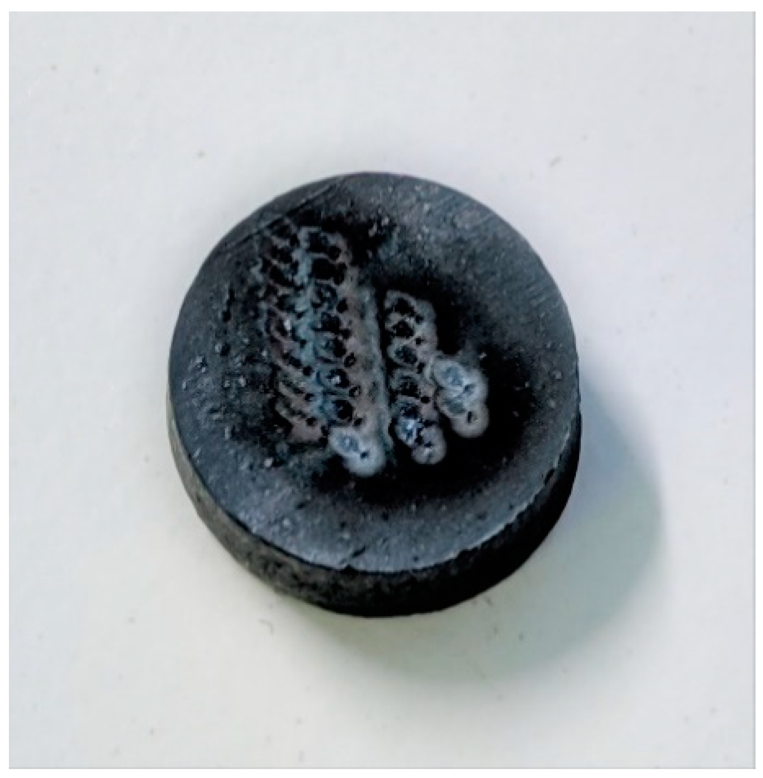
2.2. Sample Materials and LIBS Measurements

The samples were provided by Outotec and obtained from their pilot furnace. The samples consisted of ladle cooled samples, granular samples, and dip-rod samples. The ladle cooled samples were slowly cooled in the atmosphere in the ladle after collecting them from the pilot furnace whereas the granular slag samples were granulated by wet granulation. The dip rod samples were taken from inside the furnace during the ilmenite smelting and quenched immediately. Samples were selected for a wide range of TiO₂, MgO, and FeO concentrations. Seventeen samples were used during the LIBS testing, all of which were used for plasma characterization and sixteen for generating the calibration curve. The composition of the samples is mentioned in

Table 1. The concentration of analytes in slag samples analyzed by ICP-OES.

Sample (wt.%)	Mg	Ti	Fe	Mn	Si	Al
S1	6.63	32.7	12.6	0.94	0.43	0.73
S2	3.05	18.1	7.53	0.94	0.55	0.71
S3	4.67	48	3.43	1.10	0.57	1.49
S4	4.06	44.8	6.75	1.01	0.50	1.17
S5	1.03	43.6	9.93	1.19	0.57	0.97
S6	0.94	47.6	7.24	1.25	0.56	0.93
S7	0.6	39.7	4.83	1.28	0.59	0.94
S8	0.83	48.7	6.37	1.06	0.41	0.89
S9	0.92	46	11.4	1.10	0.40	0.83
S10	0.89	52	6.58	1.15	0.39	0.85
S11	0.97	50	6.63	1.18	0.45	0.85
S12	4.6	46.3	4.14	1.07	1.15	2.28
S13	4.49	44.8	3.94	1.07	1.19	2.23
S14	4.96	48	1.87	0.99	1.06	2.32
S15	0.61	51.4	4.37	0.93	0.51	0.90
S16	0.64	52.7	3.92	0.85	0.51	1.06
S17	2.66	44.5	8.35	1.00	0.53	1.09

which was obtained by inductively coupled plasma-optical emission spectrometry (ICP-OES). The LIBS spectra of the seventeen samples can be found in the Supplementary Materials in Table S1.

Each sample was turned into a fine powder using ball milling and then made into pellets of 8 mm diameter using a hydraulic press machine at 400 MPa for 5 min. Pellets prevent laser scattering and result in better LIBS spectra collection. Then they were dried in an oven for 6 h at 110 °C. The height of the samples varied from 3.3 to 7.3 mm. The sample height was not uniform to simulate the fluctuations occurring in the industrial sample preparation. As the heights of the samples were different, the samples were divided into five batches and the focal length of the LIBS set up was fixed for each batch. One major limitation of the LIBS method is that it is a surface analysis technique with an ability to analyze only a few millimeters of depth with multiple shots [18]. As the samples were crushed and mixed before pressing, the surface of the sample is considered as a uniform mixture of the bulk sample from industrial slag. To further increase the uniformity throughout the sample, LIBS spectra were obtained at 8 different positions on each sample surface. To avoid the effect of shot to shot fluctuation of the laser, each LIBS spectrum was obtained by accumulating 10 laser pulses of 6 mJ pulse energy and 5 ns duration each. At each position, the first shot was the cleaning shot to remove any oxide layer formed on the sample surface which was followed by 10 laser shots. Thus, each sample had 88 laser pulses for getting the final spectrum for the sample. Figure 2 shows the pellet sample and the pits formed by the laser shots on the top surface.

3. Results and Discussion

3.1. Plasma Characterization

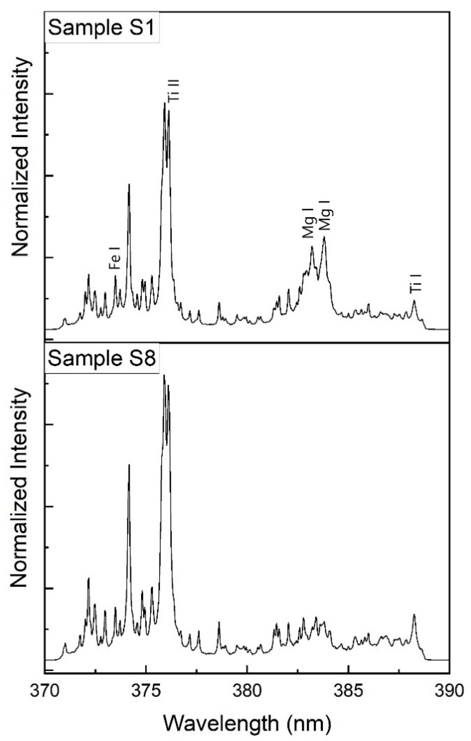
The plasma characterization was done to find out the plasma temperature and electron density for every sample. The description of the plasma characterization methods can be found elsewhere [19]. The average plasma temperature lies between 13,000 and 16,000 K during the signal acquisition, for the samples considered for study (S1–S16), which is reasonable for a LIBS plasma. The emission lines used for the plasma temperature calculations are Fe(I) 371.993, Fe(I) 380.534, Fe(I) 380.67, Fe(I) 382.782, and Fe(I) 385.991 nm. The Ti electron density of the lased induced plasma ranged from 9 × 10¹⁷ to 4 × 10¹⁸ cm⁻³ as tabulated in

Table 2. Plasma electron temperature and plasma electron density of the samples during LIBS.

Serial No.	Sample Name	Electron Temperature (K, Fe)	R2	Error (%)	Ti Plasma Electron Density (1/cm3)	Ti LTE Density (1/cm3)
1	S1	13,760.687	0.972	10.872	1.42 × 1018	6.8883 × 1015
2	S2	13,368.814	0.982	10.563	1.562 × 1018	6.7895 × 1015
3	S3	14,806.654	0.897	11.699	2.274 × 1018	7.1453 × 1015
4	S4	14,989.253	0.912	11.843	2.238 × 1018	7.1892 × 1015
5	S5	13,587.076	0.952	10.735	1.403 × 1018	6.8447 × 1015
6	S6	13,518.851	0.953	10.681	1.323 × 1018	6.8275 × 1015
7	S7	14,673.382	0.947	11.593	2.335 × 1018	7.113 × 1015
8	S8	15,028.007	0.951	11.873	2.587 × 1018	7.1985 × 1015
9	S9	15,585.366	0.950	12.314	2.934 × 1018	7.3307 × 1015
10	S10	13,543.478	0.951	10.701	1.084 × 1018	6.8337 × 1015
11	S11	15,561.469	0.943	12.295	3.288 × 1018	7.3251 × 1015
12	S12	13,164.656	0.935	10.401	9.77 × 1017	6.7374 × 1015
13	S13	15,869.721	0.932	12.539	4.06 × 1018	7.3973 × 1015
14	S14	13,777.532	0.892	10.886	1.267 × 1018	6.8925 × 1015
15	S15	15,330.347	0.977	12.112	3.163 × 1018	7.2705 × 1015
16	S16	15,196.106	0.959	12.006	3.028 × 1018	7.2386 × 1015
17	S17	17,867.997	0.950	14.117	1.227 × 1019	7.8492 × 1015

. The emission lines used for the calculation of electron density and local thermodynamic equilibrium (LTE) were Ti(I) 372.164 and Ti(II) 372.981 nm. For LTE to hold, the electron density must be higher than the LTE density [20]. It can be seen in the table that the electron density values are higher than the LTE density values, thus suggesting that the plasma is in LTE according to electron densities.

Sample S17 has higher plasma temperature and electron density compared to other samples in consideration, which is why it is not included in the calibration study. Various samples were grouped for the LIBS measurement based on the sample heights as all the samples prepared were not of identical dimensions, thus affecting the focal length of the incoming laser beam. Sample S17 was the only sample in its group and had a different focal length, which probably influenced the measured spectra. Other factors that might have resulted in a higher value of plasma temperature and electron density could be the surface condition of the sample or difference in optical set up for the sample. When included in the calibration curve, the S17 tends to give an outlier and hence was neglected for the calibration curve.

3.2. LIBS Spectra

The spectral range window centered at 380 nm was chosen for the analysis as the emission lines of Fe, Ti, and Mg could be measured simultaneously in that range. Figure 3 shows the averaged spectrum of slag Samples S1 and S8 within the wavelength range of 370 to 390 nm. Slag contains many chemical elements which makes it a complex sample containing hundreds of atomic lines in LIBS spectra. The selected range, 370 to 390 nm, includes all the emission lines of the important components (Ti, Fe, and Mg).

The difference in the composition of Samples S1 and S8 can be identified in the spectral intensity in Figure 3. S1 has high Mg content which can be observed by higher intensities of peaks around 383 nm (Mg I 382.935, Mg I 383.230, and Mg I 383.829 nm). Similarly, a higher content of Ti in sample S8 results in higher intensity peaks around 376 nm related to peaks Ti II 375.929 and Ti II 376.132 nm. The spectral lines of Mg, Fe, and Ti were identified based on the NIST database [21]. As mentioned earlier, the other impurities in the slags were neglected for this study and hence the corresponding spectral lines were not taken into consideration.

Table 3. List of strong element emission lines for Mg, Ti, and Fe from the slag samples.

Element	Spectral Line (nm)
Mg	382.935, 383.230, 383.829
Ti	375.929, 376.132, 381.458, 385.373, 385.814, 386.840, 387.320, 388.228
Fe	373.486, 373.713, 381.584, 382.042, 385.637, 385.991

lists some of the stronger elemental emission lines that were used for the LIBS analysis.

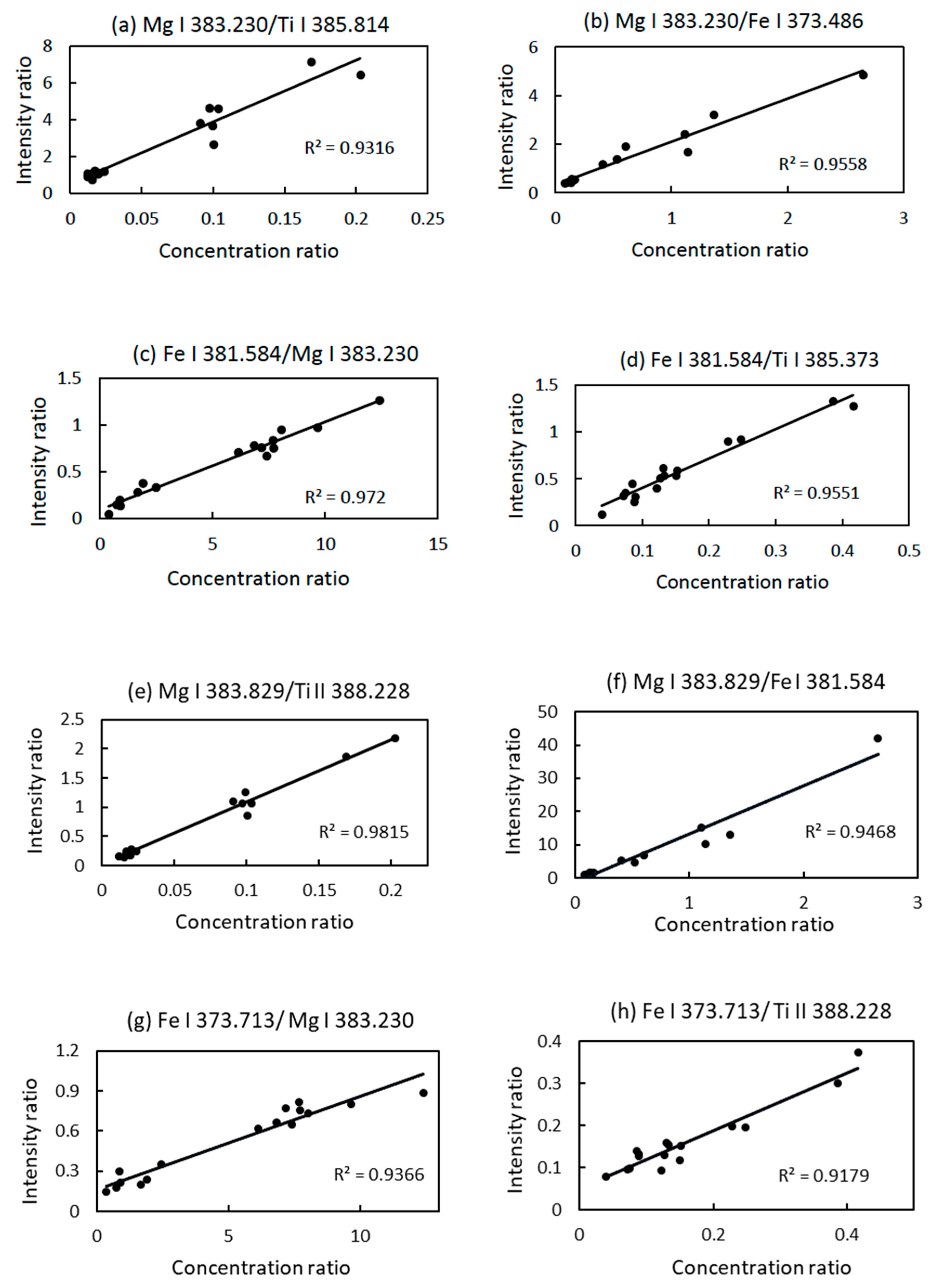
3.3. Univariate Simple Linear Regression

The intensity ratios were plotted against the concentration ratios to get the univariate calibration curve as shown in Figure 4. The correlation coefficient value, R², is between 0.93 and 0.97 for the best-fitted curves using all 16 samples, although there were outliers when other peaks were taken into consideration, which resulted in a decrease in R² value. The reason for the presence of the outlier can be attributed to the differences in the LIBS shot fluctuation and the focal distance of the laser during the experiment.

As the impurities are not taken into account, there will be a relatively higher error during the quantitative analysis of the samples using the calibration curve. The calibration curve does give an idea about the composition in terms of MgO and TiO₂ content. Samples with a high amount of MgO or less TiO₂ normally lie on the higher extreme of the calibration curve. In Figure 4a,d, Samples S1 and S2 are clustered together, where sample S1 has the highest magnesium quantity and sample S2 has the lowest titanium quantity. During the smelting operation, failure of the freeze lining in the furnace can result in a high amount of MgO in the slag, which can be represented on the calibration curve. The normal content of MgO in industrial slag is between 1 and 2%. The three clusters seen in Figure 4a can be co-related to the different content of MgO in the sample. The lowest value represents the samples with a MgO concentration of less than 1.5%, the cluster of data points in the center represents a MgO concentration of 5 to 8%, and the highest one for MgO over 10%. These values are dependent on the concentration of TiO₂ too and stand true if the concentration of TiO₂ is in the common range of 75 to 90% which is the nominal concentration in industrial slag [1].

If the impurities are neglected and the slag is assumed to just have three components of titanium, magnesium, and iron then the elemental composition can be normalized to find the composition of TiO₂ from the LIBS spectral data. Peak ratios of Mg I 383.829/Ti II 388.228, Mg I 383.829/Fe I 381.584, Fe I 381.584/Mg I 383.230, and Fe I 381.584/Ti I 385.373 were used to calculate the elemental quantity of Ti, Mg, and Fe. The results are tabulated in

Table 4. Comparative result of ICP-OES and LIBS elemental analysis and error calculation.

Sample Name	ICP-OES			LIBS			Absolute Error			% Error
	Ti	Mg	Fe	Ti	Mg	Fe	Ti	Mg	Fe	Ti	Mg	Fe
S1	0.630	0.128	0.243	0.622	0.118	0.259	−0.007	−0.009	0.016	1.15	7.21	6.79
S2	0.631	0.106	0.263	0.642	0.111	0.247	0.010	0.005	−0.015	1.66	4.52	5.81
S3	0.856	0.083	0.061	0.858	0.081	0.061	0.002	−0.002	0.000	0.26	2.55	0.19
S4	0.806	0.073	0.121	0.805	0.079	0.116	−0.001	0.006	−0.005	0.10	8.05	4.19
S5	0.799	0.019	0.182	0.781	0.018	0.201	−0.018	−0.001	0.019	2.22	4.57	10.23
S6	0.853	0.017	0.130	0.853	0.013	0.135	−0.001	−0.004	0.005	0.09	25.23	3.86
S7	0.880	0.013	0.107	0.902	0.010	0.089	0.022	−0.003	−0.018	2.48	25.69	17.21
S8	0.871	0.015	0.114	0.841	0.019	0.140	−0.030	0.004	0.026	3.49	27.74	23.05
S9	0.789	0.016	0.195	0.773	0.021	0.206	−0.016	0.005	0.011	1.99	30.37	5.59
S10	0.874	0.015	0.111	0.869	0.016	0.115	−0.006	0.001	0.005	0.66	7.38	4.23
S11	0.868	0.017	0.115	0.860	0.018	0.122	−0.008	0.001	0.007	0.93	5.11	6.30
S12	0.841	0.084	0.075	0.849	0.095	0.056	0.007	0.012	−0.019	0.88	14.03	25.45
S13	0.842	0.084	0.074	0.886	0.066	0.048	0.044	−0.018	−0.026	5.23	21.43	35.08
S14	0.875	0.090	0.034	0.905	0.086	0.009	0.030	−0.005	−0.025	3.41	5.04	74.23
S15	0.912	0.011	0.078	0.887	0.012	0.101	−0.025	0.002	0.023	2.73	15.51	29.95
S16	0.920	0.011	0.068	0.912	0.012	0.076	−0.008	0.001	0.007	0.92	10.46	10.67

with the percentage error for each sample set. To evaluate the performance of the calibration curve to achieve the quantitative measure, the root mean square error (RMSE) was calculated. RMSE is defined by:

$$\mathrm{RMSE}=\sqrt{\frac{{{\displaystyle \sum }}_{i=1}^N{\left({\widehat{y}}_i-y_i\right)}^2}{N}}$$

(1)

where ${\widehat{y}}_i$ corresponds to the reference value of the concentration of sample i, $y_i$ is the value predicted using the univariate calibration curve, and N is the number of samples.

The absolute error is the least for magnesium when compared to iron and titanium. The root mean square error (RMSE) for magnesium, iron, and titanium are 0.0067, 0.0166, and 0.0191 respectively, suggesting that it predicts magnesium with the highest accuracy. The accuracy of iron and titanium is good too and can be helpful to determine a rough estimate of the slag composition. A slag with low FeO and high Ti₂O₃ is sometimes related to foaming incidents and therefore makes it important to keep FeO content within the permissible limit. The percentage error is significantly higher for magnesium and iron for some samples than titanium. This variation can be caused by the small quantity of magnesium and iron when compared to titanium, since a small change in a component results in higher percentage error. The selection of other peak ratios gave similar results to the errors mentioned in Table 4 and can be used for calculation.

In addition to the univariate simple linear regression, partial least square (PLS) regression is a multivariate regression technique to find a relation between the peak intensity and concentration of various components. The biggest difference between PLS and univariate simple linear regression is that in the latter the intensity of single lines are compared to each other, while in the former the signal strengths are used as they are. As the univariate simple regression uses the data set directly, for a small data set it is favored over other complex regression techniques. The data set for this study is small which justifies the use of univariate simple regression in addition to the varying focal length of the LIBS setup. Some potential experimental setup improvements that can minimize the error include automatization of the lens translation stage to keep the focal point constant, the use of a control loop for the energy of the laser to limit fluctuations, and/or the use of a translation stage for the detection fiber to spatially scan the plasma. Good accuracy is achieved with the univariate analysis and can be improved further with more statistical data analysis. This confirms that the LIBS technique and the univariate and multivariate methods of analysis is a promising approach for process control of ilmenite slag, which can be applicable for other metallurgical processes as well.

4. Conclusions

In this work, the elemental analysis of ilmenite slag samples is reported using laser-induced breakdown spectroscopy (LIBS). The industrial slag samples were provided by Outotec for the investigation of Fe, Mg, and Ti content. The characteristic lines (Fe, Mg, and Ti) of LIBS spectra for the slag samples can be identified based on the NIST database. Plasma characterization was done to find the plasma temperature and electron density for each sample. The quantitative analysis for major components was done using the univariate calibration curve and was compared with the ICP-OES elemental analysis. The results obtained from LIBS in this work suggest that the concentration of elements can be identified and used to classify the samples based on the MgO and FeO content. The spectral peaks for magnesium were the strongest and were distinct when compared to iron or titanium peaks. Higher content of Mg in the slag samples was easily identified in the calibration curve and the concentration of elemental titanium and iron were predicted with good accuracy. Root mean square error was calculated to validate the predictability of the univariate calibration model with ICP-OES results. Further improvements can be done to the experimental setup to reduce errors. Future work on using LIBS for ilmenite slag studies include consideration of other impurities during analysis to improve the accuracy of the calculation. Overall, the analysis demonstrates that LIBS is a capable method to analyze high titania ilmenite slag samples for qualitative and quantitative analysis.

References

1. Pistorius, P.C. Ilmenite smelting: The basics. J. S. Afr. Inst. Min. Metall. 2008, 108, 35–43. [Google Scholar]
2. Gous, M. An overview of the Namakwa Sands ilmenite smelting operations. J. S. Afr. Inst. Min. Metall. 2006, 106, 379–384. [Google Scholar]
3. Zietsman, J.H.; Pistorius, P.C. Process mechanisms in ilmenite smelting. SIAMM J. S. Afr. Inst. Min. Metall. 2004, 104, 653–660. [Google Scholar]
4. Miziolek, A.; Vincenzo, P.; Schechter, I. Laser-Induced Breakdown Spectroscopy: Fundamentals and Applications; Cambridge University Press: New York, NY, USA, 2006. [Google Scholar]
5. Adrain, R.S.; Watson, J. Laser microspectral analysis: A review of principles and applications. J. Phys. D Appl. Phys. 1984, 17, 1915–1940. [Google Scholar] [CrossRef]
6. Romero, D.; Laserna, J.J. Infrared laser ablation and atomic emission spectrometry of stainless steel at high temperatures. J. Anal. At. Spectrom. 1999, 14, 1883–1887. [Google Scholar]
7. Kolmhofer, B.P.; Pedarnig, J.D.; Praher, R.; Huber, N.; Rössler, J.H. Element analysis of complex materials by calibration-free laser-induced breakdown spectroscopy. Appl. Phys. A 2013, 112, 105–111. [Google Scholar] [CrossRef]
8. Boué-Bigne, F. Laser-induced breakdown spectroscopy and multivariate statistics for the rapid identification of oxide inclusions in steel products. Spectrochim. Acta Part B At. Spectrosc. 2016, 119, 25–35. [Google Scholar] [CrossRef]
9. Lorenzen, C.J.; Carlhoff, C.; Hahn, U.; Jogwich, M. Applications of Laser-induced Emission Spectral Analysis for Industrial Process and Quality Control. J. Anal. At. Spectrom. 1992, 7, 1029–1035. [Google Scholar] [CrossRef]
10. Wang, Z.; Deguchi, Y.; Shiou, F.; Yan, J.; Liu, J. Application of Laser-Induced Breakdown Spectroscopy to Real-Time Elemental Monitoring of Iron and Steel Making Processes. ISIJ Int. 2016, 56, 723–735. [Google Scholar] [CrossRef] [Green Version]
11. Kolmhofer, P.J.; Eschlböck-Fuchs, S.; Huber, N.; Rössler, R.; Heitz, J.; Pedarnig, J.D. Calibration-free analysis of steel slag by laser-induced breakdown spectroscopy with combined UV and VIS spectra. Spectrochim. Acta Part B At. Spectrosc. 2015, 106, 67–74. [Google Scholar] [CrossRef]
12. Zhang, T.; Wu, S.; Dong, J.; Wang, K.; Tang, H.; Yang, X.; Li, H. Quantitative and classi fi cation analysis of slag samples by laser induced breakdown spectroscopy and partial least square (PLS) methods. J. Anal. At. Spectrom. 2015, 30, 368–374. [Google Scholar] [CrossRef]
13. Ciucci, A.; Corsi, M.; Palleschi, V.; Rastelli, S.; Salvetti, A. New Procedure for Quantitative Elemental Analysis by Laser-Induced Plasma Spectroscopy. Appl. Spectrosc. 1999, 53, 960–964. [Google Scholar] [CrossRef]
14. Sturm, V.; Schmitz, H.U.; Reuter, T.; Fleige, R.; Noll, R. Fast vacuum slag analysis in a steel works by laser-induced breakdown spectroscopy. Spectrochim. Acta Part B At. Spectrosc. 2008, 63, 1167–1170. [Google Scholar] [CrossRef]
15. Zhang, T.; Liang, L.; Wang, K.; Tang, H.; Yang, X.; Duan, Y.; Li, H. A novel approach for the quantitative analysis of multiple elements in steel based on laser-induced breakdown spectroscopy (LIBS) and random forest regression (RFR). J. Anal. At. Spectrom. 2014, 29, 2323–2329. [Google Scholar] [CrossRef]
16. Motto-Ros, V.; Negre, E.; Pelascini, F.; Panczer, G.; Yu, J. Precise alignment of the collection fiber assisted by real-time plasma imaging in laser-induced breakdown spectroscopy. Spectrochim. Acta Part B At. Spectrosc. 2014, 92, 60–69. [Google Scholar] [CrossRef]
17. Negre, E.; Motto-Ros, V.; Pelascini, F.; Lauper, S.; Denis, D.; Yu, J. On the performance of laser-induced breakdown spectroscopy for quantitative analysis of minor and trace elements in glass. J. Anal. At. Spectrom. 2015, 30, 417–425. [Google Scholar] [CrossRef]
18. Jolivet, L.; Leprince, M.; Moncayo, S.; Sorbier, L.; Lienemann, C.P.; Motto-Ros, V. Review of the recent advances and applications of LIBS-based imaging. Spectrochim. Acta Part B At. Spectrosc. 2019, 151, 41–53. [Google Scholar] [CrossRef]
19. Pauna, H.; Willms, T.; Aula, M.; Echterhof, T.; Huttula, M.; Fabritius, T. Pilot-scale AC electric arc furnace plasma characterization. Plasma Res. Express 2019, 1, 035007. [Google Scholar] [CrossRef]
20. Aragón, C.; Aguilera, J.A. Characterization of laser induced plasmas by optical emission spectroscopy: A review of experiments and methods. Spectrochim. Acta Part B At. Spectrosc. 2008, 63, 893–916. [Google Scholar] [CrossRef]
21. Kramida, A.; Ralchenko, Y.; Reader, J.; The NIST ASD Team. NIST Atomic Spectra Database (ver. 5.7); 2019. Available online: http://physics.nist.gov/asd (accessed on 15 December 2019). [CrossRef]
Figure 1. Schematic diagram of the laser ablation experiment.
Minerals 10 00855 g001
Figure 2. A pellet sample of 8 mm diameter was used as a sample for LIBS measurements.
Minerals 10 00855 g002
Figure 3. LIBS spectrum of Samples S1 (high Mg content) and S8 (low Mg content) slag samples.
Minerals 10 00855 g003
Figure 4. Simple linear calibration curve for various peak ratios (intensity ratio vs concentration ratio). (a) Mg I 383.230/Ti I 385.814, (b) Mg I 383.230/Fe I 373.486, (c) Fe I 381.584/Mg I 383.230, (d) Fe I 381.584/Ti I 385.373, (e) Mg I 383.829/Ti II 388.228, (f) Mg I 383.829/Fe I 381.584, (g) Fe I 373.713/Mg I 383.230, (h) Fe I 373.713/Ti II 388.228.
Minerals 10 00855 g004