Assessment of the Supply Chain under Uncertainty: The Case of Lithium

 , , and
Abstract
:1. Introduction
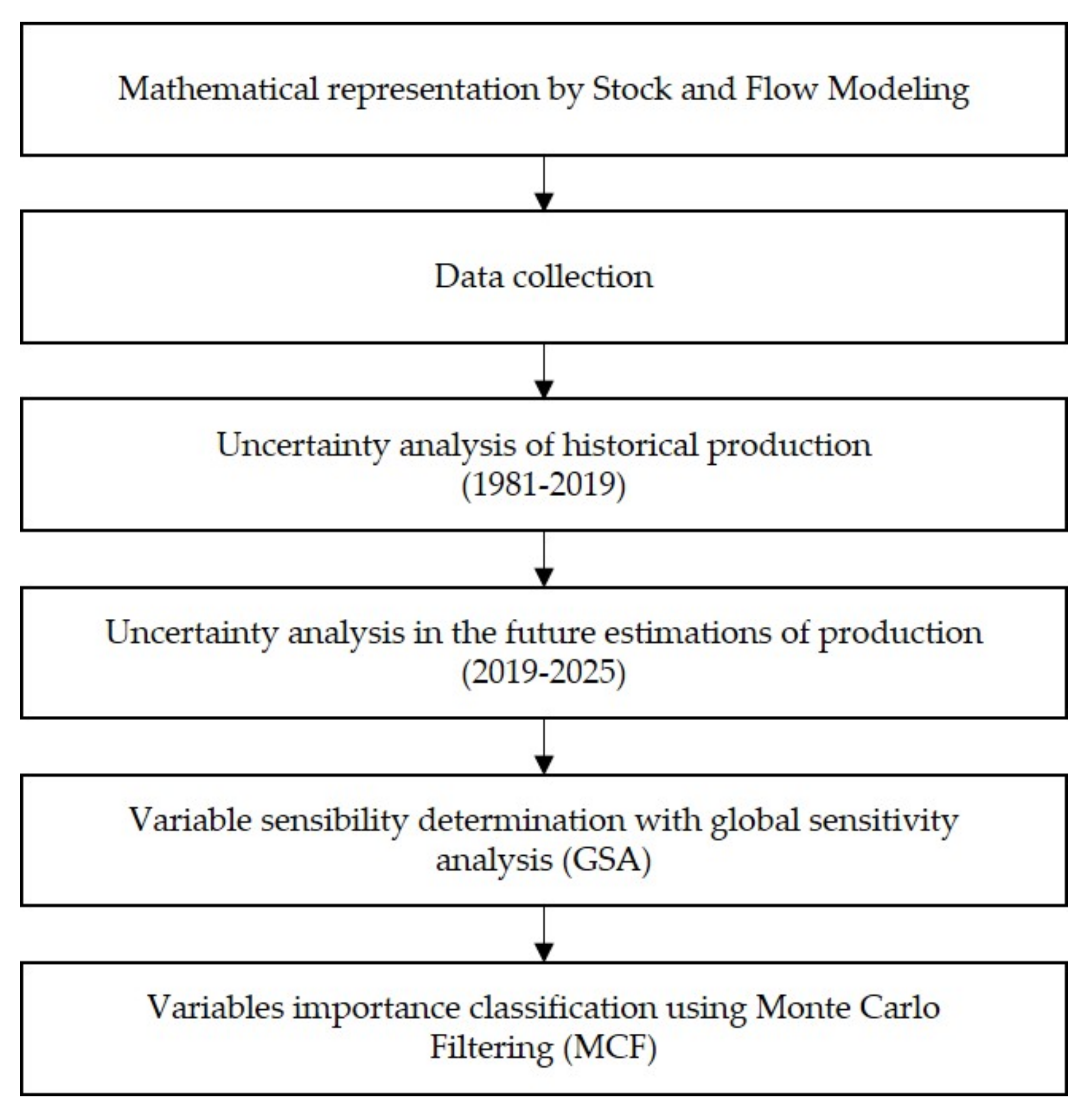
2. Methodology
2.1. Mathematical Representation by Stock and Flow Modeling
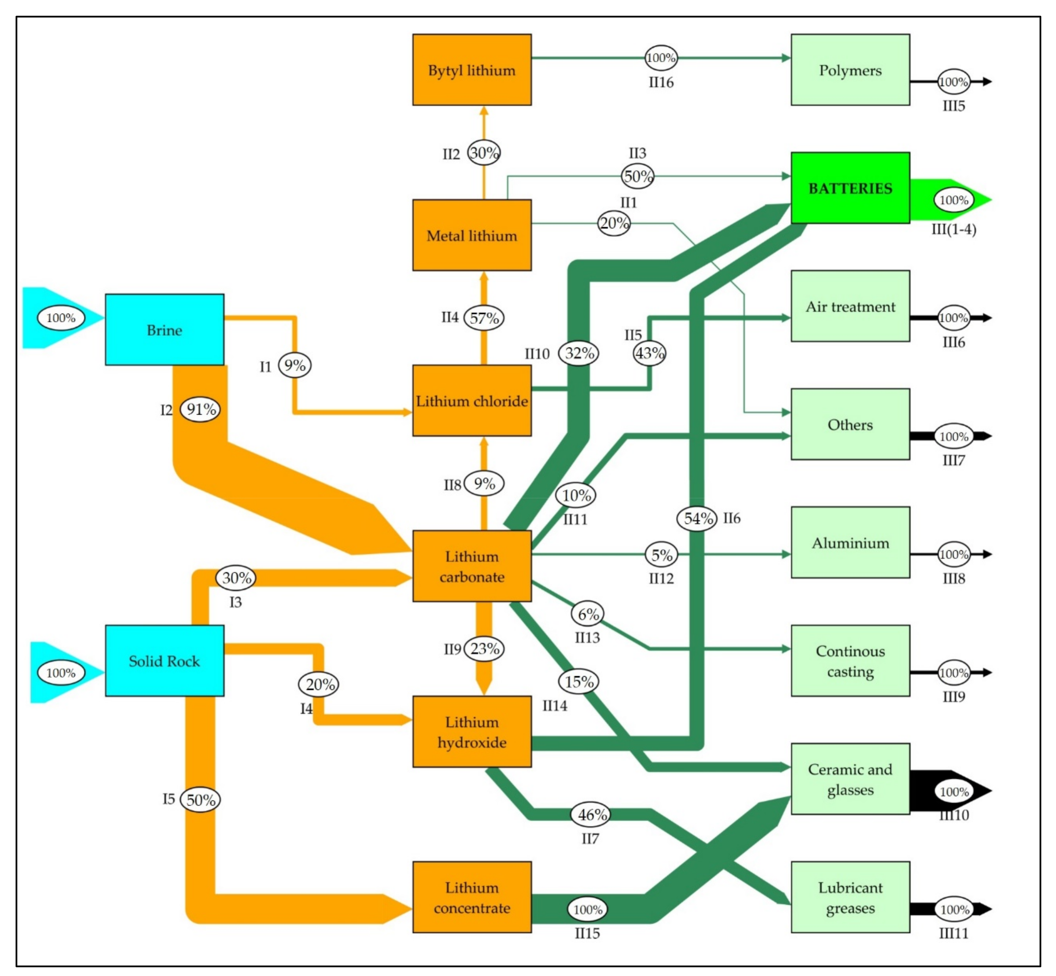
2.1.1. Conceptual Model
2.1.2. Mathematical Model
2.2. Data Collection
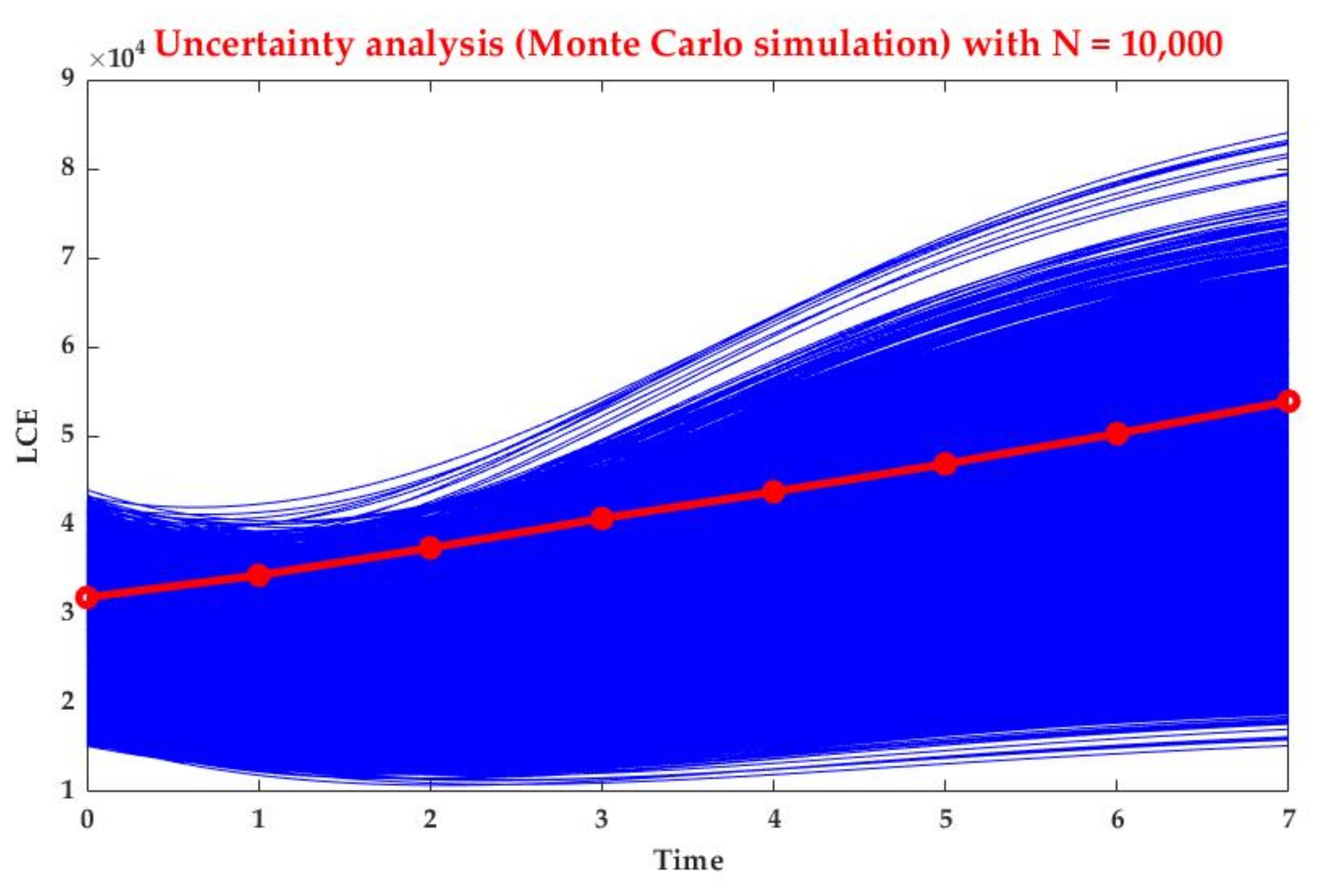
2.3. Uncertainty Analysis of Historical Production
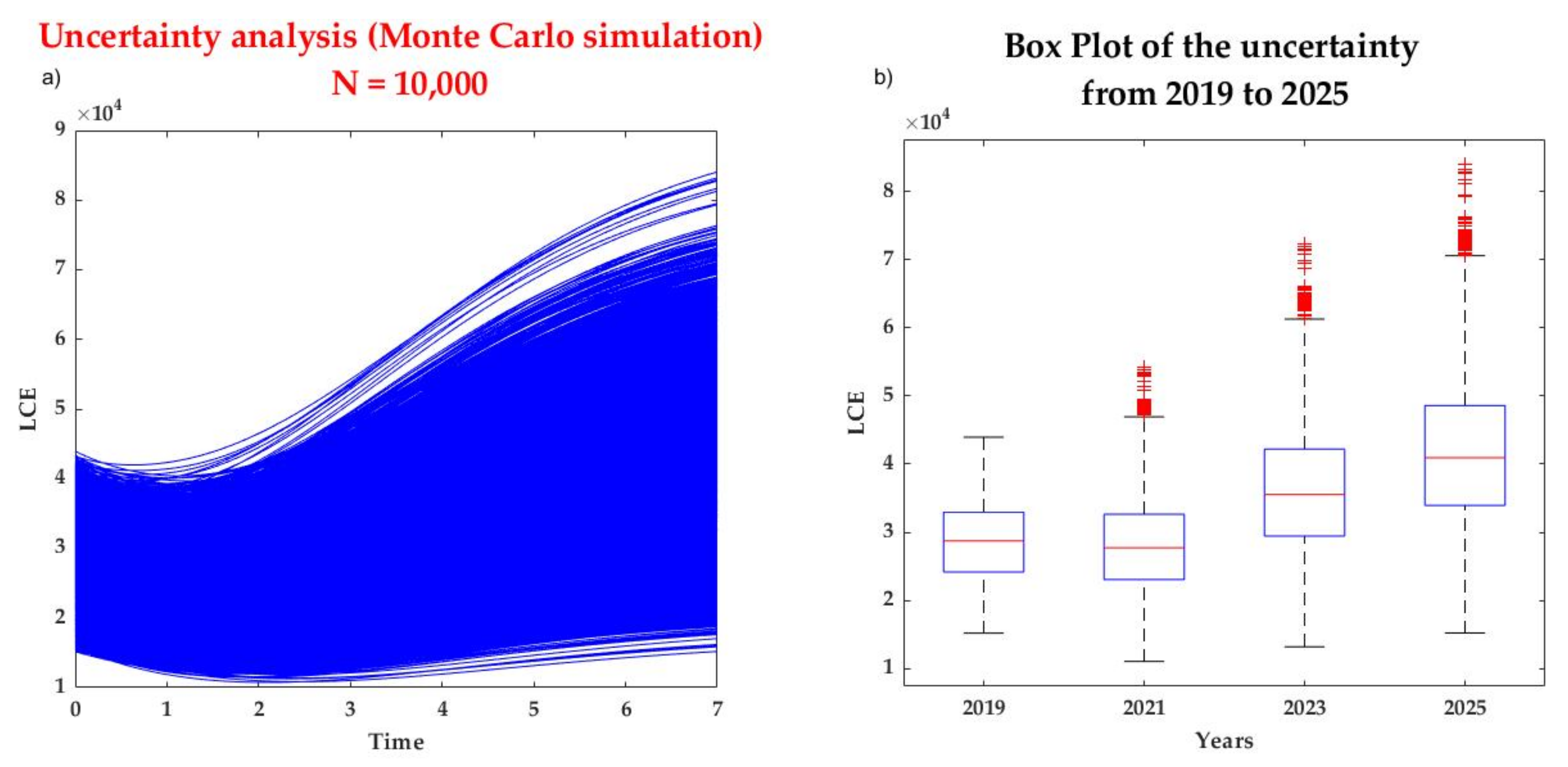
2.4. Uncertainty Analysis in the Future Estimations of Production
2.5. Variable Sensitivity Determination with Global Sensitivity Analysis (GSA)
2.6. Variable Importance Classification Using Monte Carlo Filtering (MCF)
3. Results
3.1. Mathematical Representation with Stock and Flow Modeling
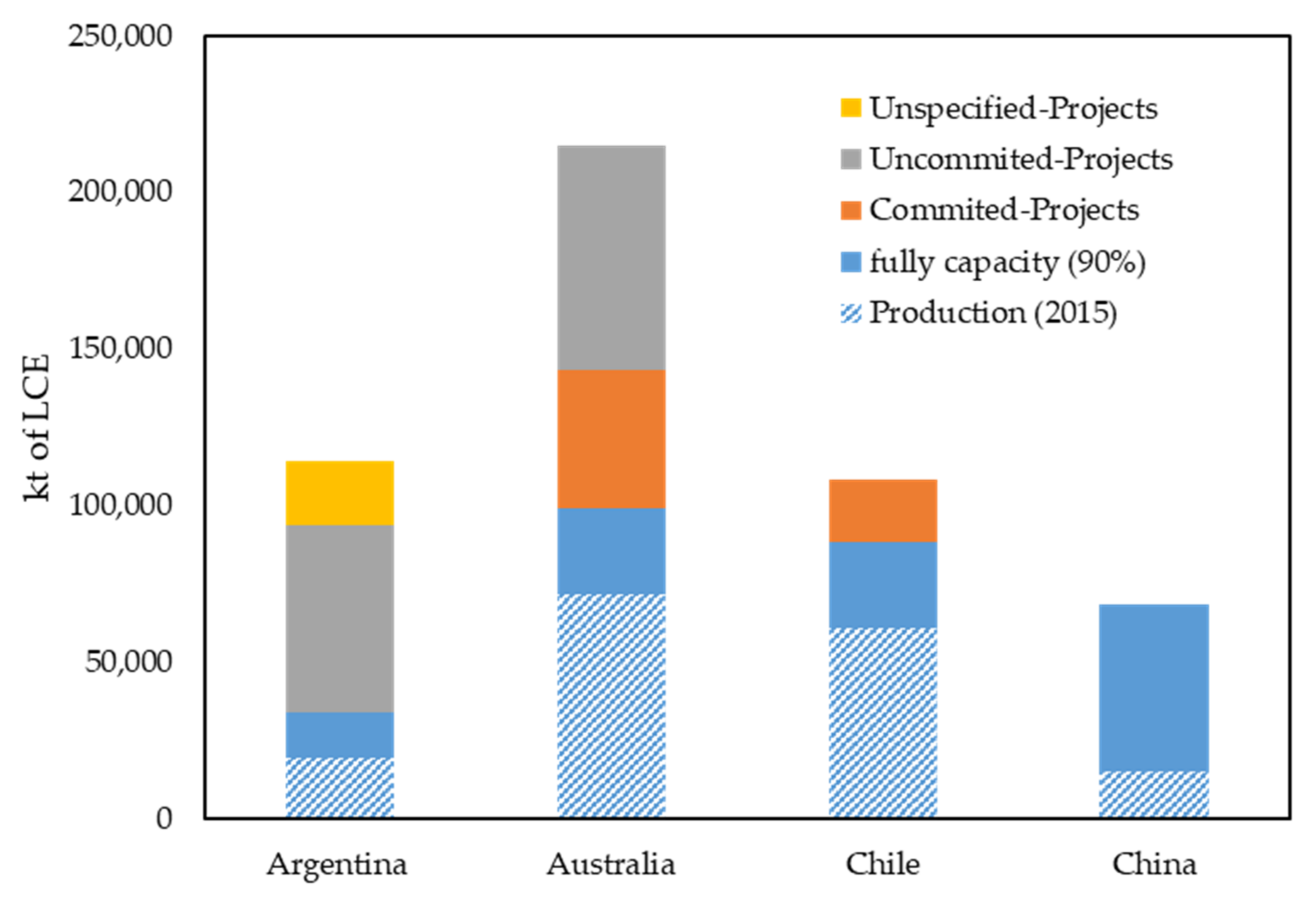
3.2. Data Collection
3.3. Uncertainty Analysis of Historical Production
3.4. Uncertainty Analysis for the Future Estimations of Production
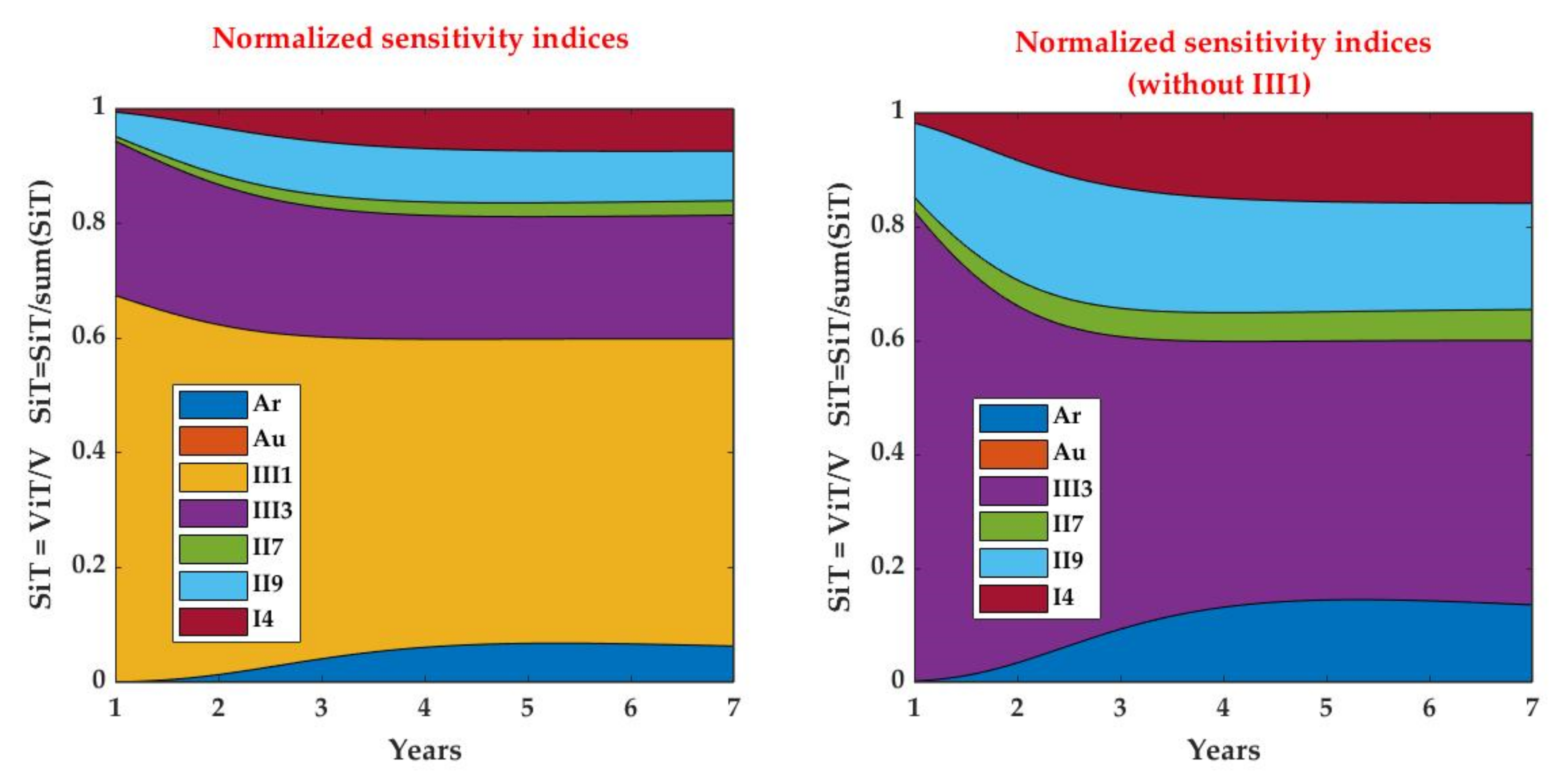
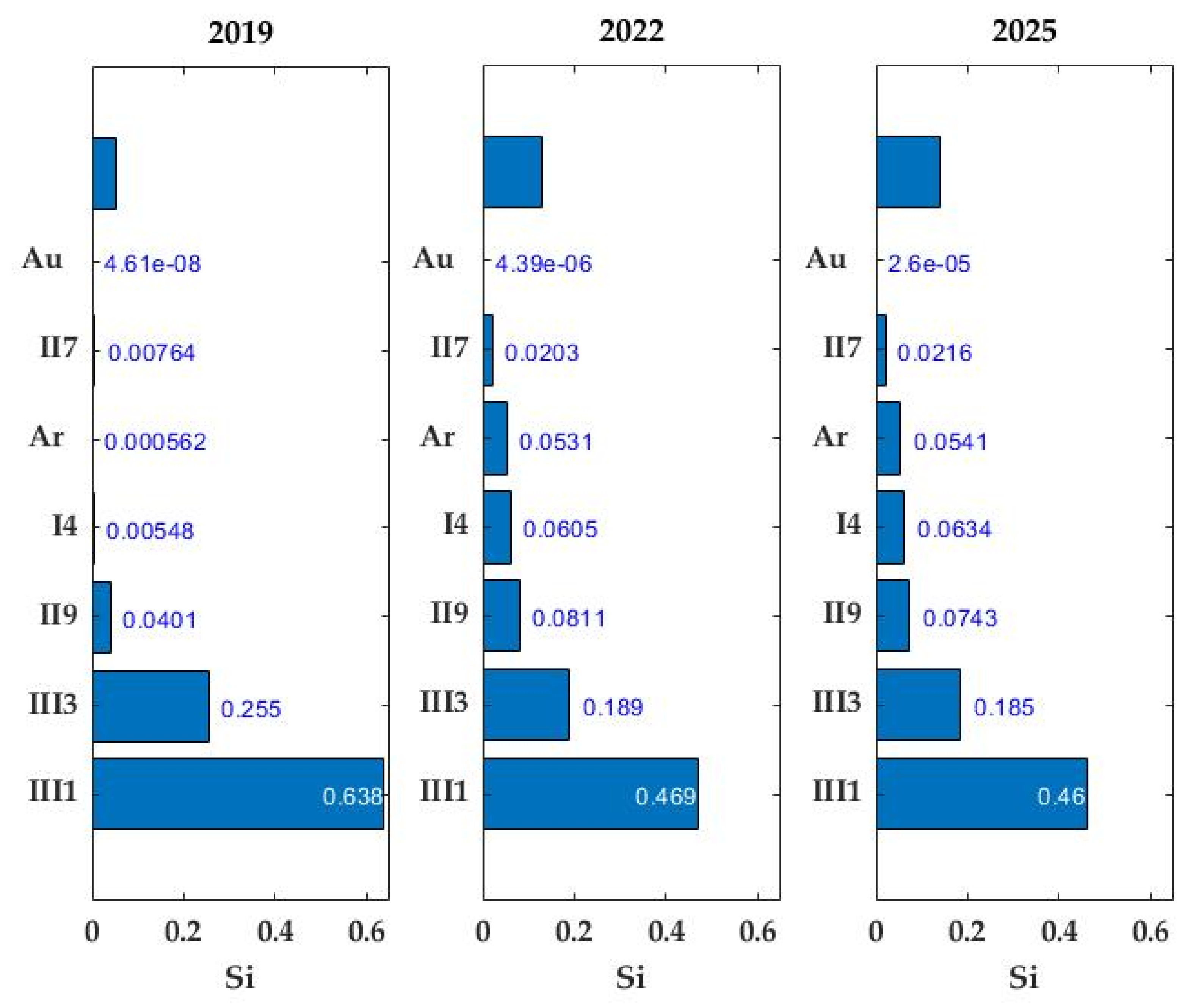
3.5. Determination of the Most Sensitive Variables with GSA
3.6. Selection of the Most Important Variables Using MCF
4. Discussion
5. Conclusions and Future Recommendations
Author Contributions
Funding
Conflicts of Interest
References
- De Koning, A.; Kleijn, R.; Huppes, G.; Sprecher, B.; van Engelen, G.; Tukker, A. Metal supply constraints for a low-carbon economy? Resour. Conserv. Recycl. 2018, 129, 202–208. [Google Scholar] [CrossRef]
- Jaskula, B. USGS Science for a Changing World. Available online: https://www.usgs.gov/centers/nmic/lithium-statistics-and-information (accessed on 1 April 2020).
- Hocking, M.; Kan, J.; Young, P.; Terry, C.; Begleiter, D. Lithium 101; Deutsche Bank Markets Research: Frankfurt, Germany, 2016. [Google Scholar]
- Staiger, J.; Roedel, T. Lithium Report 2018; Swiss Resource Capital: Herisau, Switzerland, 2018; Volume 67. [Google Scholar]
- Dalen, P. Understanding the Differences Between Deterministic and Stochastic Models. Available online: https://www.linkedin.com/pulse/understanding-differences-between-deterministic-stochastic-paul-dalen (accessed on 3 July 2020).
- Hao, H.; Liu, Z.; Zhao, F.; Geng, Y.; Sarkis, J. Material flow analysis of lithium in China. Resour. Policy 2017, 51, 100–106. [Google Scholar] [CrossRef]
- Sun, X.; Hao, H.; Zhao, F.; Liu, Z. Tracing global lithium flow: A trade-linked material flow analysis. Resour. Conserv. Recycl. 2017, 124, 50–61. [Google Scholar] [CrossRef]
- Sun, X.; Hao, H.; Zhao, F.; Liu, Z. Global Lithium Flow 1994–2015: Implications for Improving Resource Efficiency and Security. Environ. Sci. Technol. 2018, 52, 2827–2834. [Google Scholar] [CrossRef] [PubMed]
- Kim, H.; Jang, Y.; Hwang, Y.; Ko, Y.; Yun, H. End-of-life batteries management and material flow analysis in South Korea. Front. Environ. Sci. Eng. 2018, 12, 3. [Google Scholar] [CrossRef]
- Ziemann, S.; Weil, M.; Schebek, L. Tracing the fate of lithium—The development of a material flow model. Resour. Conserv. Recycl. 2012, 63, 26–34. [Google Scholar] [CrossRef]
- Chang, T.C.; You, S.J.; Yu, B.S.; Yao, K.F. A material flow of lithium batteries in Taiwan. J. Hazard. Mater. 2009, 163, 910–915. [Google Scholar] [CrossRef] [PubMed]
- Sun, X.; Hao, H.; Hartmann, P.; Liu, Z.; Zhao, F. Supply risks of lithium-ion battery materials: An entire supply chain estimation. Mater. Today Energy 2019, 14, 100347. [Google Scholar] [CrossRef]
- Speirs, J.; Contestabile, M. The Future of Lithium Availability for Electric Vehicle Batteries. In Behaviour of Lithium-Ion Batteries in Electric Vehicles; Springer: Berlin, Germany, 2018; pp. 35–57. [Google Scholar]
- Brown, T.; Walters, A.; Idoine, N.; Gunn, G.A.; Shaw, R.; Rayner, D. Lithium; British Geological Survey: Nottingham, UK, 2016. [Google Scholar]
- Brown, T. Measurement of mineral supply diversity and its importance in assessing risk and criticality. Resour. Policy 2018, 58, 202–218. [Google Scholar] [CrossRef]
- Spencer, R.; Hill, L. Specialty Minerals and Metals Industry Overview; Canaccord Genuity: Vancouver, BC, Canada, 2016. [Google Scholar]
- Gruber, P.W.; Medina, P.A.; Keoleian, G.A.; Kesler, S.E.; Everson, M.P.; Wallington, T.J. Global lithium availability. J. Ind. Ecol. 2011, 15, 760–775. [Google Scholar] [CrossRef]
- Miedema, J.H.; Moll, H.C. Lithium availability in the EU27 for battery-driven vehicles: The impact of recycling and substitution on the confrontation between supply and demand until 2050. Resour. Policy 2013, 38, 204–211. [Google Scholar] [CrossRef]
- Lowe, M.; Tokuoka, S.; Trigg, T.; Gereffi, G. Lithium-Ion Batteries for Electric Vehicles: The US Value Chain; Center on Globalization, Governance & Competitiveness, Duke University Press: Durham, NC, USA, 2010. [Google Scholar]
- Notter, D.A.; Gauch, M.; Widmer, R.; Wager, P.; Stamp, A.; Zah, R.; Althaus, H.-J. Contribution of Li-ion batteries to the environmental impact of electric vehicles. Environ. Sci. Tehnol. 2010, 44, 6550–6556. [Google Scholar] [CrossRef]
- Martin, G.; Rentsch, L.; Hoeck, M.; Bertau, M. Lithium market research—Global supply, future demand and price development. Energy Storage Mat. 2017, 6, 171–179. [Google Scholar] [CrossRef]
- Ballinger, B.; Stringer, M.; Schmeda-Lopez, D.R.; Kefford, B.; Parkinson, B.; Greig, C.; Smart, S. The vulnerability of electric vehicle deployment to critical mineral supply. Appl. Energy 2019, 255, 113844. [Google Scholar] [CrossRef]
- Pehlken, A.; Albach, S.; Vogt, T. Is there a resource constraint related to lithium ion batteries in cars? Int. J. Life Cycle Assess. 2017, 22, 40–53. [Google Scholar] [CrossRef]
- Lucay, F.A.; Gálvez, E.D.; Salez-Cruz, M.; Cisternas, L.A. Improving milling operation using uncertainty and global sensitivity analyses. Miner. Eng. 2019, 131, 249–261. [Google Scholar] [CrossRef]
- Clift, R.; Druckman, A. Taking Stock of Industrial Ecology; Springer: Berlin, Germany, 2016; ISBN 9783319205700. [Google Scholar]
- Jaskula, B.W. Lithium, Minerals Yearbook-2015; US Geological Survey: Reston, VA, USA, 2017; pp. 41–44. [Google Scholar]
- Müller, E.; Hilty, L.M.; Widmer, R.; Schluep, M.; Faulstich, M. Modeling Metal Stocks and Flows: A Review of Dynamic Material Flow Analysis Methods. Environ. Sci. Technol. 2014. [Google Scholar] [CrossRef]
- Glöser, S.; Soulier, M.; Espinoza, L.T.; Faulstich, M. Using Dynamic Stock & Flow Models for Global and Regional Material and Substance Flow Analysis in the Field of Industrial Ecology: The Example of a Global Copper Flow Model. In Proceedings of the 31st International Conference of the System Dynamics Society, Cambridge, MA, USA, 21–25 July 2013. [Google Scholar]
- Emilia, S. Dynamic Modelling of Material Flows and Sustainable Resource Use Case Studies in Regional Metabolism and Space Life Support Systems Emilia Suomalainen; Université de Lausanne: Lausanne, Switzerland, 2012. [Google Scholar]
- Gerst, M.; Graedel, T.E. In-Use Stocks of Metals: Status and Implications. Environ. Sci. Technol. 2008, 42. [Google Scholar] [CrossRef]
- Hodge, A.; Crowley, B.; Bairstow, H.; Ljubisavljevic, S.; Hamilton, C.; Morton, P.; Kejriwal, D.; May, C.; Diyachkina, P.; South, F.; et al. Global Lithium Report; Macquarie Group Limited: Sydney, Australia, 2016. [Google Scholar]
- Foss, M.M.; Gülen, G.; Tsai, C.-H.; Quijano, D.; Elliott, B. Battery Materials Value Chains; Center for Energy Economics (CEE): Austin, TX, USA, 2015. [Google Scholar]
- Helton, J.C.; Oberkampf, W.L. Alternative representations of epistemic uncertainty. Reliab. Eng. Syst. Saf. 2004, 85, 1–10. [Google Scholar] [CrossRef]
- Rowe, W.D. Understanding uncertainty. Risk Anal. 1994, 14. [Google Scholar] [CrossRef]
- Helton, J.C.; Burmaster, D.E. Treatment of aleatory and epistemic uncertainty in performance assesments for complex systems. Reliab. Eng. Syst. Saf. 1996, 54, 91–94. [Google Scholar] [CrossRef]
- Oberkampf, W. Uncertainty quantification using evidence theory. In Proceedings of the Advanced Simulation Computing Workshop, Albuquerque, MN, USA, 22–23 August 2005. [Google Scholar]
- Christian, J.; Van Der Sluijs, J.P.; Lajer, A.; Vanrolleghem, P.A. Uncertainty in the environmental modelling process e A framework and guidance. Environ. Model. Softw. 2007, 22, 1543–1556. [Google Scholar] [CrossRef] [Green Version]
- Casals Casals, L.; Amante García, B.; Gonzáles Benítez, M. Modelling Li-Ion Battery Aging for Second Life Business Models Lluc Canals Casals Modelling Li-Ion Battery Aging for Second Life Business Models; Universitat Politécnica de Catalunya: Barcelona, Spain, 2016. [Google Scholar]
- Richa, K.; Babbitt, C.W.; Gaustad, G.; Wang, X. A future perspective on lithium-ion battery waste flows from electric vehicles. Resour. Conserv. Recycl. 2014, 83, 63–76. [Google Scholar] [CrossRef]
- Mohr, S.H.; Mudd, G.M.; Giurco, D. Lithium resources and production: Critical assessment and global projections. Minerals 2012, 2, 65–84. [Google Scholar] [CrossRef]
- Morgan, M.G.; Henrion, M. A Guide to Dealing with Uncertainty in Quantitative Risk and Policy Analysis; Cambridge University Press: Cambridge, UK, 2007; ISBN 9780521365420. [Google Scholar]
- Brunner, H.; Rechberger, P. Practical Handbook of Material Flow Analysis; Lewis Publishers: Boca Raton, FL, USA, 2005; ISBN 1566706041. [Google Scholar]
- Saltelli, A.; Trantola, S.; Campolongo, F.; Ratto, M. Sensitivity Analysis in Practice; Wiley: Hoboken, NJ, USA, 2004; ISBN 0470870931. [Google Scholar]
- Lilburne, L.; Tarantola, S. Sensitivity analysis of spatial models. Int. J. Geogr. Inf. Sci. 2009, 23, 151–168. [Google Scholar] [CrossRef] [Green Version]
- Saltelli, A.; Annoni, P.; Azzini, I.; Campolongo, F.; Ratto, M.; Tarantola, S. Variance based sensitivity analysis of model output. Design and estimator for the total sensitivity index. Comput. Phys. Commun. 2010, 181, 259–270. [Google Scholar] [CrossRef]
- Lucay, F.A.; Lopez-Arenas, T.; Sales-Cruz, M.; Gálvez, E.D.; Cisternas, L.A. Performance Profiles for Benchmarking of Global Sensitivity Analysis Algorithms. Rev. Mex. Ing. Química 2020, 19, 423–444. [Google Scholar] [CrossRef] [Green Version]
- Saltelli, A.; Ratto, M.; Andres, T.; Campolongo, F.; Cariboni, J.; Gatelli, D.; Saisana, M.; Tarantola, S. Global Sensitivity Analysis. The Primer; John Wiley & Sons, Ltd.: Chichester, UK, 2007; ISBN 9780470725184. [Google Scholar]
- Grosjean, C.; Herrera, P.; Perrin, M.; Poggi, P. Assessment of world lithium resources and consequences of their geographic distribution on the expected development of the electric vehicle industry. Renew. Sustain. Energy Rev. 2012, 16, 1735–1744. [Google Scholar] [CrossRef]
- Wendl, M.; Wietschel, M.; Marscheider-Weidemann, F.; Angerer, I.G. Abschätzung des Künftigen Angebot-Nachfrage-Verhältnisses von Lithium vor dem Hintergrund des Steigenden Verbrauchs in der Elektromobilität; Karlsruhe Institut für Technologie: Karlsruhe, Germany; Fraunhofer-Institut für System-und Innovationsforschung: Karlsruhe, Germany, 2009. [Google Scholar]
- Jaskula, B.W. Lithium, Minerals Yearbook-2014; US Geological Survey: Reston, VA, USA, 2016; pp. 41–44.
- Vikström, H.; Davidsson, S.; Höök, M.; Sonoc, A.; Jeswiet, J.; Idjis, H.; Attias, D.; Bocquet, J.C.; Richet, S. A review of lithium supply and demand and a preliminary investigation of a room temperature method to recycle lithium ion batteries to recover lithium and other materials. Procedia CIRP 2013, 110, 252–266. [Google Scholar]


| Country | 2015 Production Capacity |
|---|---|
| Argentina | 51% |
| Australia | 65% |
| Chile | 62% |
| China | 20% |
| Parameters of the Uniform Distribution | ||||
|---|---|---|---|---|
| Supply Chain Stage | Distribution Variable | Path | Min a | Max b |
| Stage I | DV-I1 | Brine to LiCl | 4% | 10% |
| DV-I2 | Brine to Li2CO3 | 53% | 91% | |
| DV-I3 | Solid rock to Li2CO3 | 27% | 47% | |
| DV-I4 | Solid rock to LiOH | 4% | 45% | |
| DV-I5 | Solid rock to Lithium concentrate | 33% | 90% | |
| Parameters of Uniform Distribution | ||||
|---|---|---|---|---|
| Supply Chain Stage | Distribution Variable | Path | Min a | Max b |
| Stage II | DV-II1 | Metallic lithium to others | 22% | 25% |
| DV-II2 | Metallic lithium to butylithium | 56% | 70% | |
| DV-II3 | Metallic lithium to batteries | 22% | 50% | |
| DV-II4 | LiCl to lithium metallic | 30% | 64% | |
| DV-II5 | LiCl to air treatment | 36% | 36% | |
| DV-II6 | LiOH to batteries | 29% | 59% | |
| DV-II7 | LiOH to lubricants | 24% | 50% | |
| DV-II8 | Li2CO3 to LiCl | 7% | 10% | |
| DV-II9 | Li2CO3 to LiOH | 15% | 30% | |
| DV-II10 | Li2CO3 to batteries | 21% | 44% | |
| DV-II11 | Li2CO3 to others | 9% | 11% | |
| DV-II12 | Li2CO3 to aluminum | 1% | 9% | |
| DV-II13 | Li2CO3 to continuous casting molds | 5% | 8% | |
| DV-II14 | Li2CO3 to ceramics | 11% | 19% | |
| Parameters of Uniform Distribution | ||||
|---|---|---|---|---|
| Supply Chain Stage | Distribution Variable | Path | Min a | Max b |
| Stage III | DV-III1 | Batteries to electric vehicles | 17% | 45% |
| DV-III2 | Batteries to energy storage systems (ESS) | 1% | 5% | |
| DV-III3 | Batteries to traditional batteries | 30% | 62% | |
| DV-III4 | Batteries to two wheeler electric vehicles | 4% | 10% | |
| Variables with Uncertainty | Description |
|---|---|
| III1 | Distribution from batteries to electric vehicles |
| Au | The Australian production of lithium |
| III3 | Distribution from batteries to traditional batteries |
| II9 | Distribution from lithium carbonate to lithium hydroxide |
| II7 | Distribution from lithium hydroxide to lubricants |
| Ar | Argentinian production of lithium |
| I4 | Distribution from pegmatite to lithium hydroxide |
| Variable | Year | ||||
|---|---|---|---|---|---|
| 2017 | 2019 | 2021 | 2023 | 2025 | |
| III1 Batt_EV | crucial | crucial | crucial | crucial | important |
| Australia | insignificant | insignificant | insignificant | insignificant | insignificant |
| III3 Batt_Tbatt | crucial | crucial | crucial | crucial | crucial |
| II9 LCE_LiOH | crucial | crucial | important | important | important |
| II7 LiOH_Lub | important | crucial | crucial | important | insignificant |
| Argentina | insignificant | crucial | crucial | important | insignificant |
| I4 Solid Rock _LiOH | important | crucial | crucial | important | crucial |
© 2020 by the authors. Licensee MDPI, Basel, Switzerland. This article is an open access article distributed under the terms and conditions of the Creative Commons Attribution (CC BY) license (http://creativecommons.org/licenses/by/4.0/).
Share and Cite
Calisaya-Azpilcueta, D.; Herrera-Leon, S.; Lucay, F.A.; Cisternas, L.A. Assessment of the Supply Chain under Uncertainty: The Case of Lithium. Minerals 2020, 10, 604. https://doi.org/10.3390/min10070604
Calisaya-Azpilcueta D, Herrera-Leon S, Lucay FA, Cisternas LA. Assessment of the Supply Chain under Uncertainty: The Case of Lithium. Minerals. 2020; 10(7):604. https://doi.org/10.3390/min10070604
Chicago/Turabian StyleCalisaya-Azpilcueta, Daniel, Sebastián Herrera-Leon, Freddy A. Lucay, and Luis A. Cisternas. 2020. "Assessment of the Supply Chain under Uncertainty: The Case of Lithium" Minerals 10, no. 7: 604. https://doi.org/10.3390/min10070604