Abstract
Random noise is unavoidable in seismic data acquisition due to anthropogenic impacts or environmental influences. Therefore, random noise suppression is a fundamental procedure in seismic signal processing. Herein, a deep denoising convolutional autoencoder network based on self-supervised learning was developed herein to attenuate seismic random noise. Unlike conventional methods, our approach did not use synthetic clean data or denoising results as a training label to build the training and test sets. We directly used patches of raw noise data to establish the training set. Subsequently, we designed a robust deep convolutional neural network (CNN), which only depended on the input noise dataset to learn hidden features. The mean square error was then evaluated to establish the cost function. Additionally, tied weights were used to reduce the risk of over-fitting and improve the training speed to tune the network parameters. Finally, we denoised the target work area signals using the trained CNN network. The final denoising result was obtained after patch recombination and inverse operation. Results based on synthetic and real data indicated that the proposed method performs better than other novel denoising methods without loss of signal quality loss.
1. Introduction
Seismic signals are often disturbed by noise, and consequently, the signal-to-noise ratio (SNR) of seismic signals is typically low. A low SNR indicates poor signal quality, which affects downstream signal processing, such as deconvolution [1], seismic in-version [2], and seismic attribute analysis [3]. Therefore, seismic signals must be pre-processed to obtain clear and high-resolution seismic profiles [4,5], and effective noise removal methods are critical for seismic signal pre-processing [6,7]. The relationship between noise and signals is typically classified as coherent and incoherent. Unlike incoherent noise, which is randomly mixed with the effective signal, affects signal recognition, and does not have a fixed dominant frequency or apparent velocity, coherent noise shows a correlation with effective signals, thereby enabling the identification of defined features.
Effective suppression of seismic random noise and the recovery of high-quality seismic data are challenging and have garnered considerable attention from the scientific community [8,9]. Many denoising methods and theories have been proposed and widely used in seismic data processing. The first method is based on the seismic data stack in the offset direction [10,11]. However, this method is not suitable for pre-stack seismic data denoising and exhibits considerable dip angle limitations. The second method is based on predictive filtering, which assumes that the signal is predictable and random noise is not. Based on the above theory, f–x deconvolution (FXDECON) [12,13], non-stationary predictive filtering [14], and t–x predictive filtering [15] have been proposed. Although frequency filtering suppresses regular interference waves, such as surface waves, it is not effective for random noise processing. The third method is based on mathematical transformation, which uses the differences between the signal and noise in the transform domain to better separate the signal and noise. Examples include the Fourier transform [16,17], wavelet transform [18,19], Radon transform [20], curvelet transform [21,22], dreamlet transform [23], and seislet transform [24,25]. Nevertheless, when the data features are complex, the robustness and efficiency of these algorithms must be optimal. The fourth method is based on matrix rank dimension reduction [26,27]. These methods assume that clean seismic data are low-order structures. Therefore, seismic data can be denoised by reducing the rank. One example of this approach is multi-channel singular spectrum analysis (MSSA) [28]. The fifth method is based on dictionary learning trans-formation [29,30], which constructs an over-complete dictionary for sparse decomposed signals and separates the effective signal and noise [31]. This type of algorithm entails dictionary updating and sparse coding, which is computationally complex.
More importantly, these methods must establish the noise parameters based on experience. When the parameters are not properly set, the denoising effect is relatively poor [32]. Therefore, a procedure for intelligent data processing that does not require prior knowledge is critical to establish the denoising parameters accurately and efficiently. Deep learning enables the extraction of hidden features by learning the low-level features of data, which can then be used for prediction or classification [33,34]. Thus, deep-learning algorithms [35,36] facilitate seismic random noise attenuation based on data-driven approaches. Most deep-learning methods are based on supervised learning [37] and unsupervised learning [38]. In supervised learning, training label selection is critical because it is the basis of the learning features. However, clean label data are difficult to obtain. Synthetic noiseless records [39] are often used as training labels. This approach is not suitable for the analysis of real data. The authors of [40] proposed that the denoised data obtained from traditional methods can be considered as the input of the training set; however, this limits denoising performance. The corresponding noise label cannot be obtained from real seismic data, and therefore, a real training label cannot be constructed. In contrast, unsupervised denoising enables the recovery of clean data from noisy data without the need for data labeling. An autoencoder (AE) is a neural network that is often used to extract data features [41]. Specifically, this procedure is a self-supervised learning technique that can be used for efficient data encoding. More importantly, AE has several advantages compared with other supervised learning technologies [42,43]. The authors of [44] proposed a sparse AE neural network for seismic noise attenuation. Unfortunately, the features extracted using this method are not sufficient for effective seismic data reconstruction. AE variants include the stacked AE (SAE), denoising AE (DAE), variational AE (VAE), and others. Among them, SAE stacks several AEs to form a deep structure. Greedy layer-wise learning is used to train SAE multiple times. SAE is used to discover highly nonlinear and complex features. However, in the case of weak classification, the performance of SAE degrades sharply [45,46]. DAE introduces noise into the encoding, resulting in an encoding file, which is a corrupted version of the original input data. The idea, therefore, is to force the hidden layer to acquire more robust features and to prevent the network from merely learning the identity function. DAE can be used to denoise the corrupted signal and extract the important features from the data [47]. VAE produces a probability distribution for the different features of the latent attributes. It arranges the learned features with similar shapes close to each other in the projected latent space, thereby reducing the loss in the reproduction of input. Nevertheless, an increase in the dimensionality of the latent layer without an increase in the complexity of data causes a VAE to extract unrepresentative features and to overfit the training dataset [48,49]. In practice, autoencoders are widely used for image coloring, denoising, dimensionality reduction, watermark removal, anomaly detection, and feature variation. To extract the complex characteristic of seismic data better, we modified the convolutional DAE network to provide a novel approach for exploring seismic data.
Our study aimed to suppress incoherent noise (i.e., random noise) from seismic data and improve the efficiency and robustness of convolutional AE learning. We employed unsupervised learning, as mentioned above, and proposed a deep convolutional DAE network framework to attenuate seismic random noise. Unlike traditional methods, which employ synthetic clean data or denoising results as training labels, we used raw noise data to directly construct the training set. The advantage of the proposed method was that we were able to quickly prepare the training dataset from the noisy data using any input real seismic data input, and we did not disconcert the process of obtaining the real training labeling. Our method showed excellent ability in exploring the specific characteristic of the real noisy seismic data because we designed multiple filters and special procedures for extracting useful features. The MSE was selected as an error criterion to establish the cost function. Additionally, tied weights were used to reduce over-fitting risk. These modifications accelerated the training process and the acquisition of optimal network parameters. Finally, the optimized CNN was used to denoise the patches from a target region. The final denoising result was obtained after patch synthesis and inverse operation. This method was used to process synthetic and real seismic data along with other novel denoising methods such as MSSA, FXDECON, and wavelet transform. Upon comparison, the proposed method was found to be more effective than the aforementioned alternatives.
2. Methodology
Seismic data noise was defined as the sum of the effective signal and noise and could be expressed as follows:
where X is the clean signal to be solved, N is the additive noise, and Y is the observed seismic noise data.
Y = X + N,
Notably, signal X was independent of noise N. We restricted our discussion to the assumption that the noise term N was additive isotropic Gaussian noise, and each example was a variance distribution derived from a zero-mean vector.
The proposed method, which was based on deep CNNs, primarily aimed to establish a relationship between X and Y. To train an effective deep CNN, a good training dataset and test dataset should be prepared first.
2.1. Training Set Preparation and Self-Supervised Learning
To ensure the quality of deep learning and accelerate network convergence, we first normalized the original seismic dataset Y as follows:
where is the normalized dataset, and Y.max is the maximum value of the original data. We normalized the data range to a value between −1 and 1.
2.1.1. Self-Supervised Learning
Self-supervised learning is adopted to circumvent the need for label preparation associated with supervised learning [50]. Our training data were not extracted from clean data. Instead, we directly used the noise data of the target region. The neural network was then used to extract the characteristics of the seismic data by learning a small number of training samples. Afterwards, the feature model was used to analyze the entire work area for denoising.
2.1.2. Dataset Preparation
After normalizing the data derived from the region of interest, the random sampling operator R1 was introduced to randomly extract the data from the target area to construct the training set Xtrain as follows:
where the sampling operator R1 randomly divides the noisy data Y* of the target work area into a size N × N matrix and uses cutting operator C to divide the training data into smaller training patches of size n to obtain Xtrain. This approach could generate immense training samples, which was helpful to network learning. However, using small datasets could reduce computational complexity and improve the efficiency of neural network training. After repeated experiments and referring to the literature, a total of 32 general training seismic patches (n value) were selected from a range of 28–64 [51,52].
When the entire AE network structure completed the deep-learning training for the training set Xtrain, the neural network model was used to denoise the target work area as follows:
First, the target work area was divided into N1 × N2 data using the regular operator , after which the training data was divided into smaller patches with size n using the cutting operator C for denoising. The neural network model with optimized parameters was then used to denoise and obtain after prediction. Subsequently, the denoised blocks were restored to the large data block using operator . Finally, the sampling operator was used to reverse the process and merge the data into a complete work area, after which reverse normalization was performed to obtain the denoised data of the entire work area.
The patch numbers of the training and test sets were generally different. Each patch in the training set processed by cutting operator C had the same size n as the small block in the test set. Additionally, we used operator to ensure that all raw data were included in the denoising process. The entire process is illustrated in Figure 1.

Figure 1.
Proposed workflow.
2.2. Principle of Convolutional AE Seismic Denoising
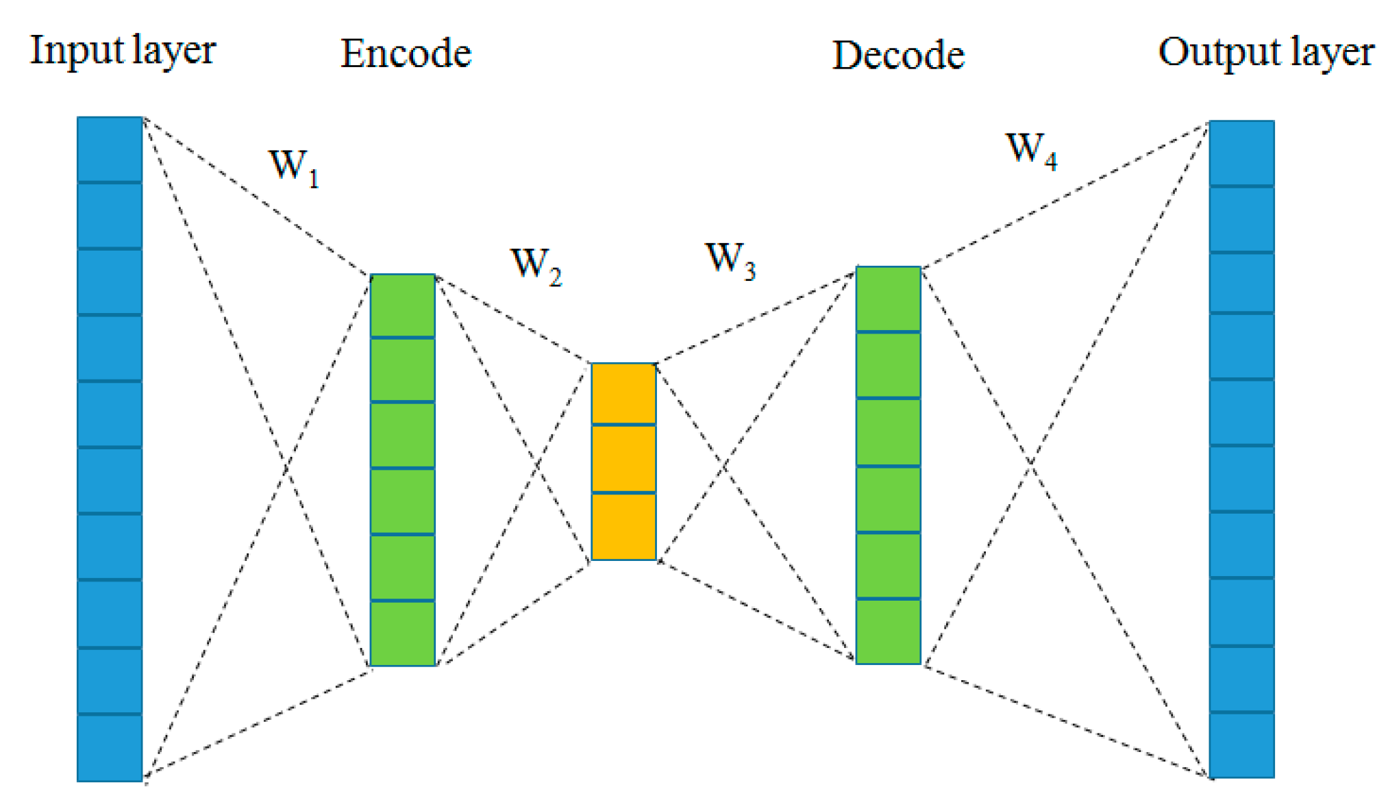
DAE neural networks were used for feature selection and extraction via dimensionality reduction and reconstruction. AE neural networks used fewer hidden layers than inputs to train the network to ignore input “noise”, as shown in Figure 2.
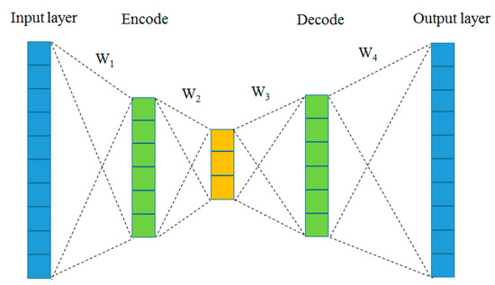
Figure 2.
Schematic of DAE neural network.
The encoding process was as follows: For the input noise data X, there was a mapping relationship F, which was used to compress X into Y. This was generally referred to as an “encoder”. Moreover, this mapping relationship was typically nonlinear.
where is a nonlinear activation function. The encoding mapping parameter is set as F = {W, b}, where W is the weight matrix, and b is the offset.
The decoding process was as follows: through a mapping relation G(Y), the compressed representation Y was restored to the reconstruction Z, which was as close as possible to its input:
where is a nonlinear activation function. The encoding mapping parameter is set as G = {W, b}, where W is the weight matrix, and b is the offset.
G(Y) = σ(W2Y + b2),
The entire encoding and decoding processes were trained by minimizing the loss function as follows:
The purpose of mapping F(x) and G(Y) was to minimize the average reconstruction error of the training set, so that Z was similar to the original input noisy data X. The parameters were initialized randomly and then optimized using the random gradient descent method.
Based on the above-described procedure, the entire DAE process consisted of data feature extraction and recovery of complete data [53]. Encoding was a dimension-reduction process that was used to extract specific features, whereas decoding was a dimension-raising process that was used to recover complete data. Since random noise was irregular data and effective signals were regular data, a robust feature representation could be generated through nonlinear neural network learning. Therefore, if an algorithm could accurately reconstruct its input, it could also retain most of the input feature information [54].
When we denoise a one-dimensional signal, a fully connected AE neural network is always selected. Nevertheless, fully connected AE neural networks were not appropriate for two-dimensional seismic signals because: (1) a fully connected AE neural network flattened the input layer and turned them into a single vector that lost the structural information of seismic signals; (2) in a fully connected mesh topology, all nodes were connected to each other, thereby resulting in considerable redundancy and prohibitively high implementation costs.
In recent years, CNNs have been successfully implemented to extract local features of multidimensional data and have shown extraordinary denoising performance. However, the complexity of seismic profile signals was considerably higher than that of ordinary images because of the complexity of the stratigraphic structure and noise interference. Therefore, our study aimed to improve the efficiency and robustness of convolutional AE learning. In this study, we proposed a modified AE neural network based on tied weights, which combined AE with CNNs to improve the performance of seismic noise attenuation and showed a higher practical application value.
2.3. Proposed Network Architecture and Optimization
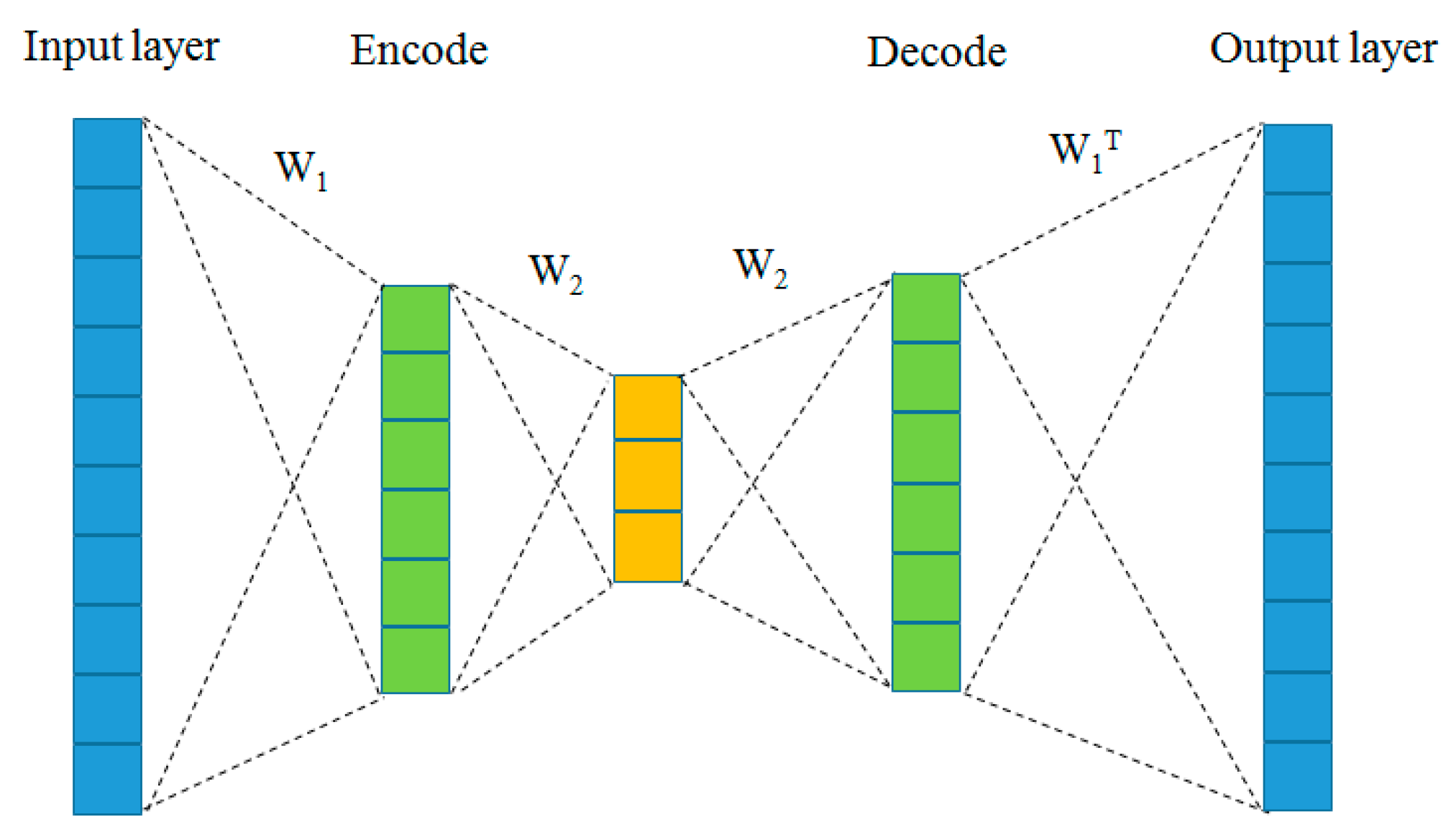
We proposed an end-to-end deep DAE network in which the encoder and decoder functions were combined. The proposed DAE requires structurally symmetric encoding and decoding layers, as shown in Figure 3. In other words, they had the same size in the corresponding structure, sharing certain parameters; therefore, only one set of weights was needed for learning. In the last layer, the decoding weight was the transpose of the first encoding weight because of the opposite process. We used the up-sampling layer to resize the signal, which simply doubled the dimensions of the input signal and did not perform an inverse operation. In the other decoding layers, the decoding weights and encoding weights shared the same set of weights. This was described using formulas (7) and (8):
where is the mapping vector of the i-th layer, and and are the weight and bias of the training, respectively. Moreover, is the nonlinear activation function, where n is the total number of convolution layers, and is the weight of the i-th convolution layer. In this way, the tied weights between the encoder and decoder are generated.
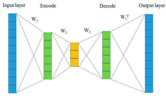
Figure 3.
Proposed DAE tied-weights neural network.
Compared with learning individual weights in the decoding and coding stages, this method had the following benefits: (1) faster training speed, as we stopped the model training process in decoding layers by freezing the weights and shared the weights from encoding layers, reducing the number of model parameters and just learning one set of weights; (2) better learning performance, as this was often preferred over learning separate weights for both phases and could be regarded as a regularisation form, thus reducing the risk of over-fitting.
Figure 4 illustrates the overall network architecture and key steps of our proposed procedure. In the entire convolutional encoding layer (L1–L3), we used three pairs of convolutional layers, batch regularisation layers, and max-pooling layers. The intermediate layer (L4) was a pair of convolution and batch regularisation layers. The intermediate layer was a latent representation layer that forced the AE to find patterns in the input data and to eliminate unimportant features. In the decoding layer (L5–L7), we used three pairs of up-sampling layers, batch regularisation layers, and convolution layers, which were mirror-symmetric to the encoding layer. In the encoding and decoding process steps, leaky ReLU was used as the activation function to enhance the training of complex seismic signals with negative values. In the last layer, tanh was used as the activation function because the range of the tanh activation function value was between −1 and 1, which was more suitable for our model. A max-pooling layer, which accelerated the calculation and prevented over-fitting, was used to obtain translation invariant representation and dimension reduction. A batch regularisation layer was used to stabilize the gradient training of deep neural networks, thereby improving training speeds [55]. In the decoding layer, the up-sampling layer was used to expand the dimensions of the hidden feature to reconstruct the original sample. This method was based on the up-sampling processing of the nearest-neighbour interpolation, which increased the sample rate by inserting zeros between samples.

Figure 4.
The architecture of our proposed method.
As mentioned above, combining Equations (1)–(11), the entire denoising process was expressed as follows:
where X represents the input noisy data, and Z represents the denoised restored data after processing. The represents the DAE neural network model, which included seven layers. indicated that the network parameters including weight and bias. We froze the weights in the decoding layers and shared the weights from encoding layers.
The size of the signal patch and convolution filter had a dramatic effect on the denoising performance of the model. Through several experiments and by referring to previous studies [44,45,46,47,48,49], we selected the best performing 32 × 32 as the best performing patch size and 3 × 3 as the filter size. We used Adam as the optimizer and MSE as the loss function. A total of 25 epochs were trained, and satisfactory results were obtained. Table 1 shows the network architecture.

Table 1.
List of hyperparameters for the proposed deep networks.
3. Numerical Experiments
The denoising performance of the proposed method was assessed using synthetic and real data, after which the results were compared with those obtained with three novel methods (wavelet transform, FXDECON, and MSSA). The denoising performance results were evaluated based on the peak signal-to-noise ratio (PSNR). This parameter represented the ratio between the maximum possible power of a signal and the destructive noise power.
PSNR was typically used to evaluate the quality of a compressed image and compare the results with the original image (used for signal denoising). The higher the value of the PSNR, the better the quality and the higher the resolution. PSNR was expressed as follows:
where MAX is the peak value of the signal and PSNR is measured in dB, which is mainly used for image compression. When processing an image, MAX represents the maximum possible pixel value. In seismic data processing, MAX is the maximum value of the seismic data.
MSE is an estimator that represents the cumulative square error between the reconstructed and original signals. The lower the MSE value, the lower the error. MSE can be expressed as follows:
where is the original data, is the approximate data (processed data), and m and n are the data dimensions.
3.1. Synthetic Seismic Signal
3.1.1. Synthetic Signal Used in the Experiment
The synthetic seismic signal used herein was part of a record obtained from the forward modeling, consisting of 120 traces with a total time of 0.6 s, and a sampling interval time of 5 ms, each of which included 120 sampling points, as shown in Figure 5a. The entire seismic signal was complex and contained both strong and weak amplitude signals. The noise signal shown in Figure 5b was obtained after normalizing the seismic signal and adding random noise levels of 0.25. The PSNR of the noise signal was 13.98 dB, which was used as the test signal in the subsequent process. The noise pollution was considerable, with fuzzy axis signals and details that were difficult to distinguish.
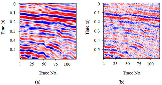
Figure 5.
Synthetic seismic signal example. (a) Clean data, (b) Noise data (PSNR = 13.98 dB).
3.1.2. Comparison between Tied Weights and Non-Tied Weights
First, we evaluated the influence of tied weights and non-tied weights on the denoising performance of synthetic data. We performed the algorithm experiment on a notebook with a 2.0 G Intel i7 8 core processor and 16 GB of memory. To verify the denoising efficiency and denoising results of the two network models, we performed tied-weights and non-tied-weights denoising experiments on seven different training sets (from 10,000 to 40,000) with the same network parameters and the same training epoch (25 epochs).
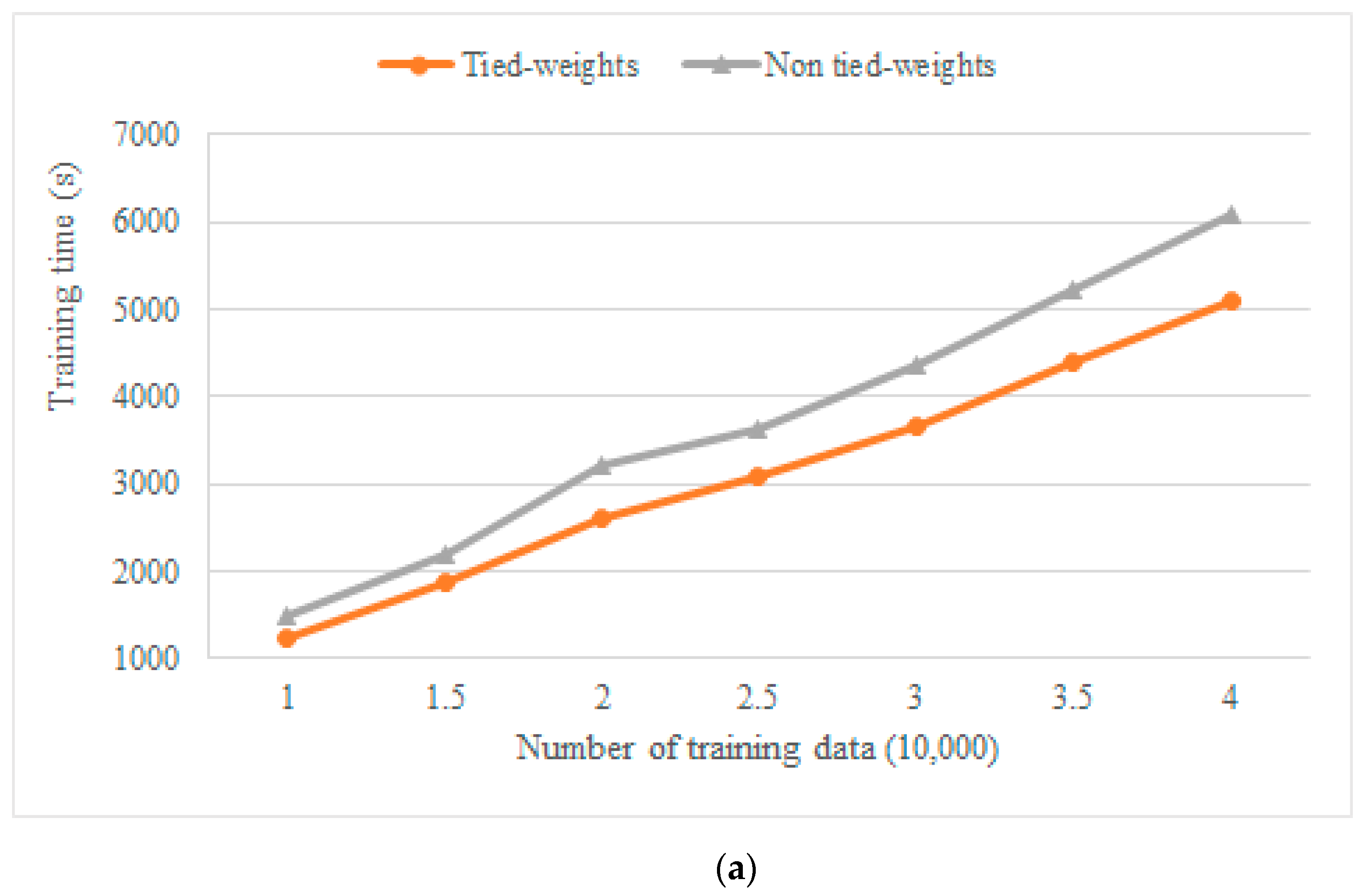
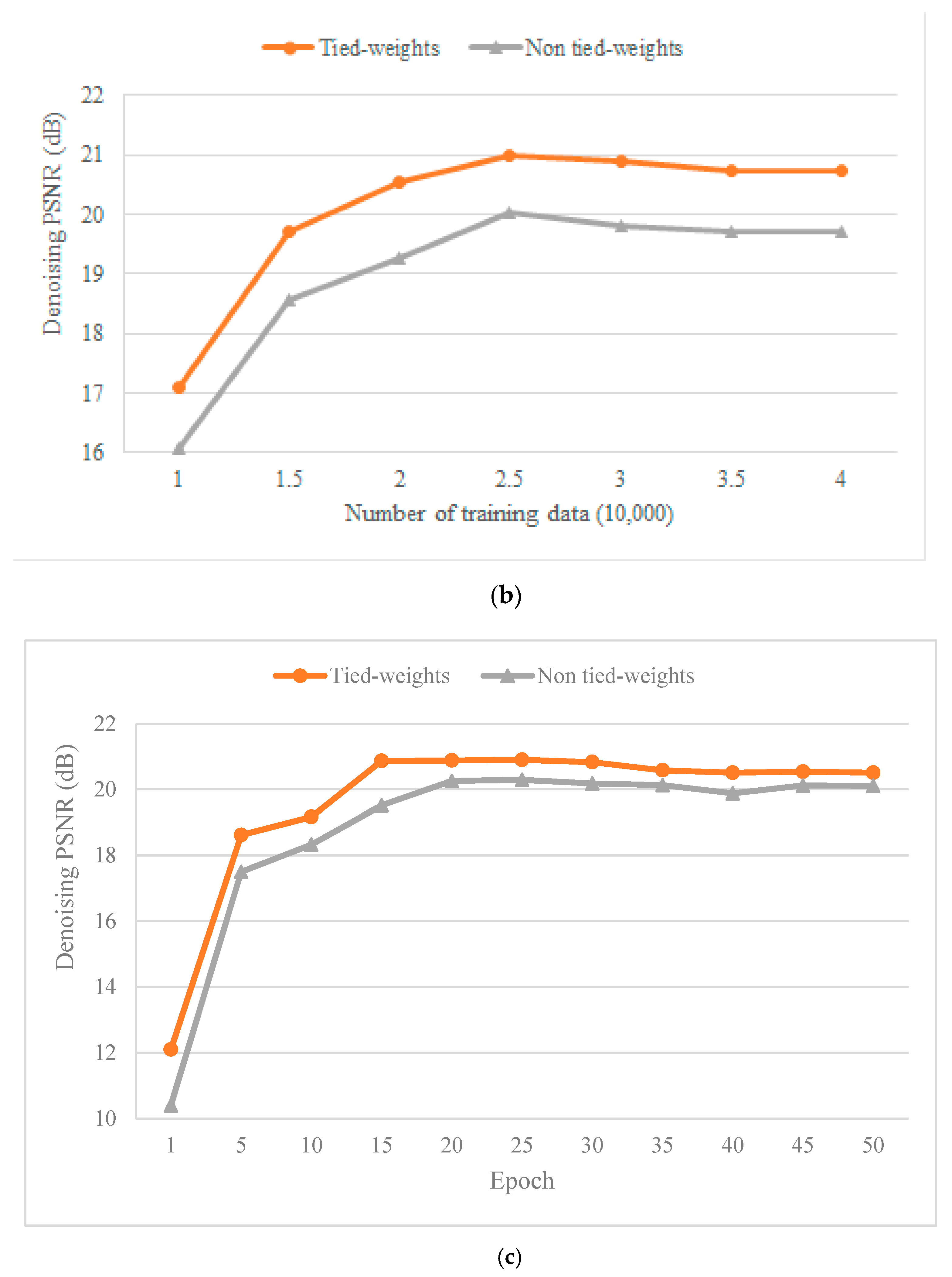
Figure 6a showed the training time of the two network models for different numbers of training sets. The training time of the tied-weights model for different numbers of training sets was lower than that of the non-tied-weights model, and the average training time was reduced by 19%, which demonstrated that the tied-weights AE method improved the training speed (Table 2). Figure 6b showed the denoising effect of the two network models after optimizing the model parameters through different numbers of training sets. We then calculated the PSNR value of the denoised result and the original clean signal. The PSNR of the tied-weights model for different numbers of training sets was higher than that of the non-tied-weights model, with an average improvement of 1.08 dB, which proved that the proposed method performed better (Table 3). The two methods achieved the best results when using 25,000 training sets, after which the denoising effect tended to be stable but not improved. Figure 6c shows the denoising effect of the two network models after optimizing the model parameters through different epochs. We also calculated the PSNR value of the denoised result and the original clean signal. First, the PSNR of the tied-weights model for different epochs was higher than that of the non-tied-weights model with an average improvement of 0.80 dB, which proved that the proposed method performed well (Table 4). Second, the two methods achieved the best results after 25 epochs, after which the denoising effect tended to be stable but not improved. In other words, 25 epochs led to the best denoising performance.

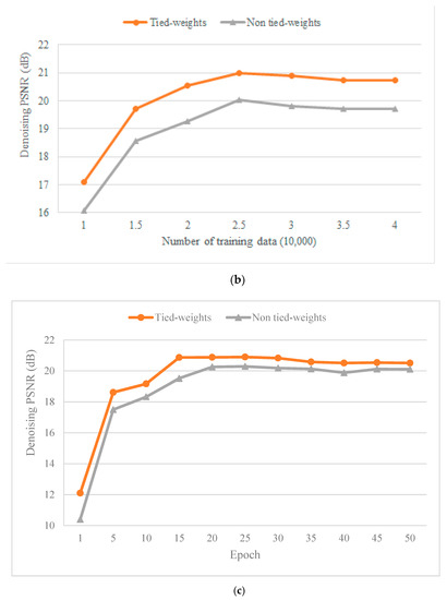
Figure 6.
Comparison of tied-weights and non-tied-weights processing results. (a) Training time comparison with respect to the training number. (b) Denoising result comparison with respect to the training number. (c) Denoising result comparison with respect to epochs. The red line represents the tied-weights AE model, and the grey line represents the non-tied-weights AE model.

Table 2.
Training time comparison with respect to training number of tied weights and non-tied weights.

Table 3.
Denoising results with respect to the training number of tied weights and non-tied weights.

Table 4.
Denoising results with respect to the epochs of tied weights and non-tied weights.
3.1.3. Experimental Comparison with Other Denoising Algorithms
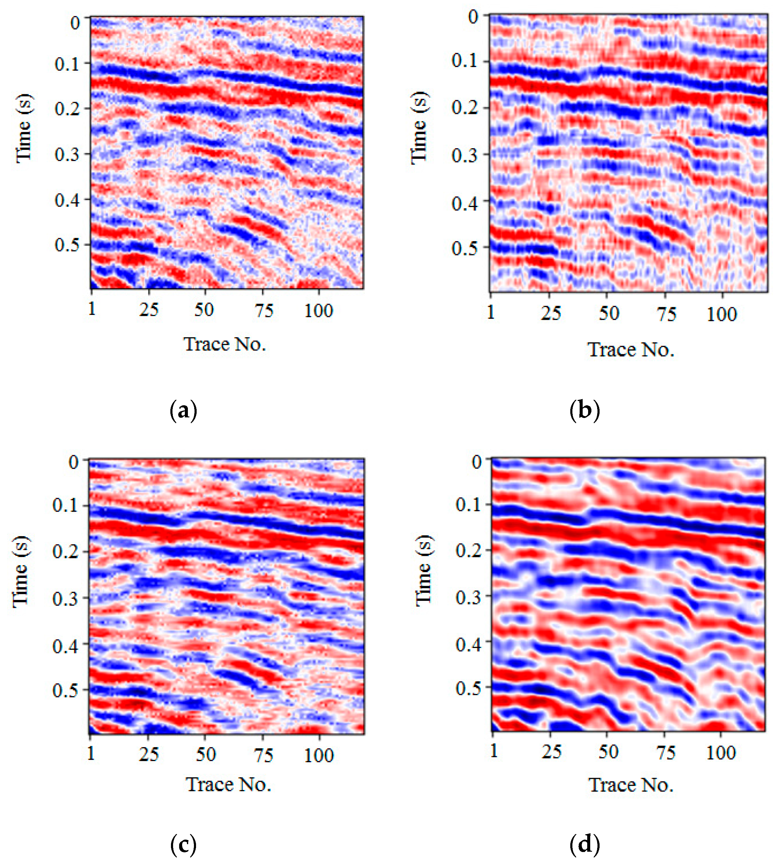
We compared the existing three novel denoising algorithms, FXDECON, MSSA, and wavelet transform, with our proposed methods. As shown in Figure 7, some random noise was still observed in a–c, and the edge of the event axis was fuzzy. In Figure 7d, random noise interference was almost absent, and the edge of the event axis of the effective signal became clear. The results illustrated in Figure 7d demonstrated that the PSNR value of our proposed method was 21.00 dB, which was higher than the denoising results of other methods. Table 5 shows the main parameters and denoising performance of each method. Therefore, both the qualitative and quantitative results demonstrated that the denoising ability of the proposed method was better than that of the other three methods.
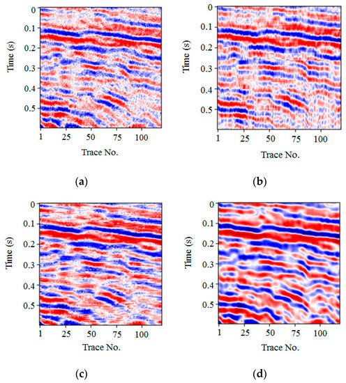
Figure 7.
Denoised result comparison for synthetic data. Denoise results using (a) FXDECON (PSNR = 16.77 dB), (b) MSSA (PSNR = 15.01 dB), (c) wavelet transform (PSNR = 17.63 dB), and (d) the proposed method (PSNR = 21.00 dB).

Table 5.
Quantitative evaluation of FXDECON, MSSA, wavelet transform, and the proposed methods. Parameters are tuned manually.
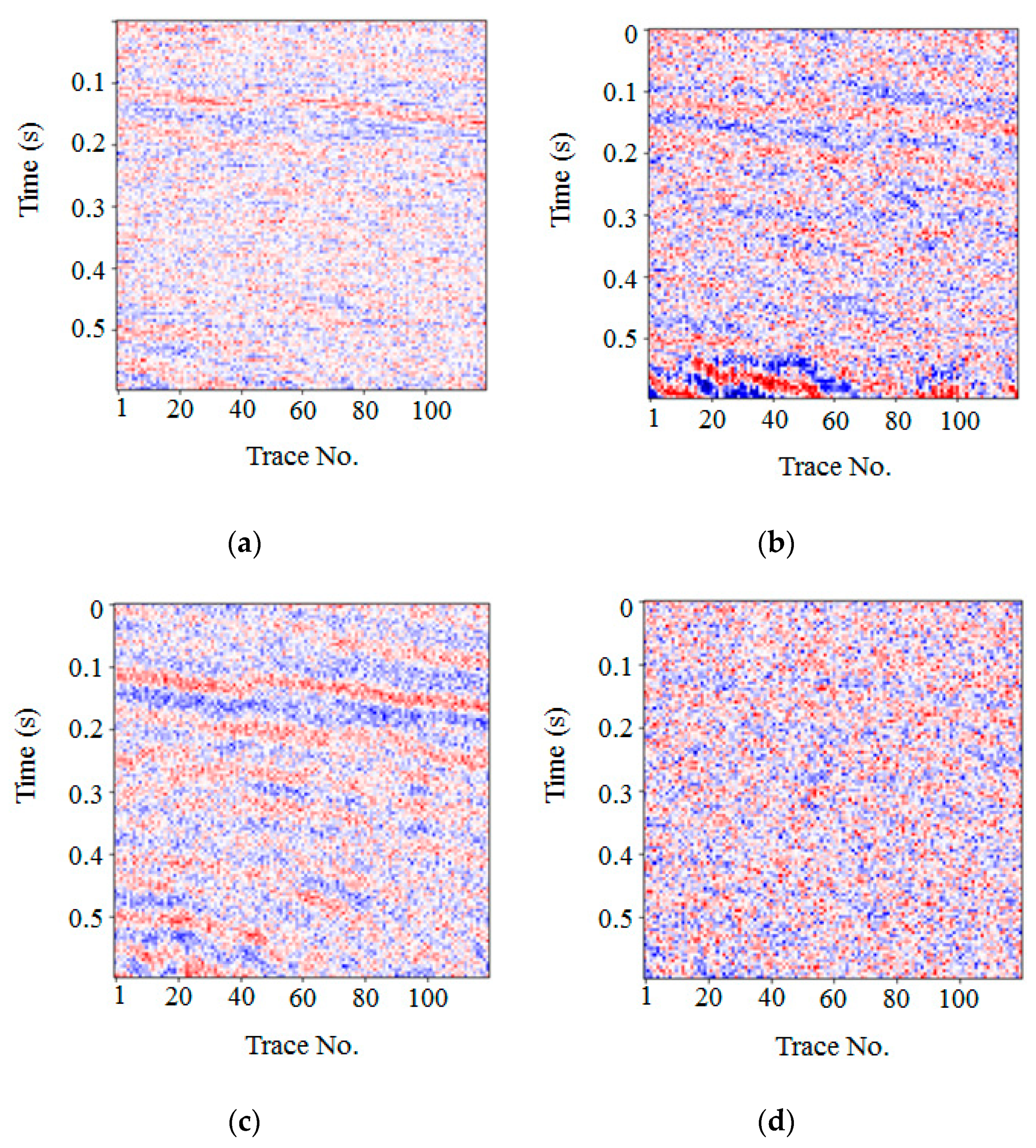
Figure 8 illustrates the noise removal results of the FXDECON, MSSA, wavelet transform, and the proposed method. Fewer random noise and residual effective signals were observed in Figure 8a, whereas 8b and 8c removed more random noise but left some residual effective signals. In Figure 8d, more random noise was removed, but fewer residual coherent signals were left. This illustrated that the proposed method could remove more random noise while maintaining an effective signal.
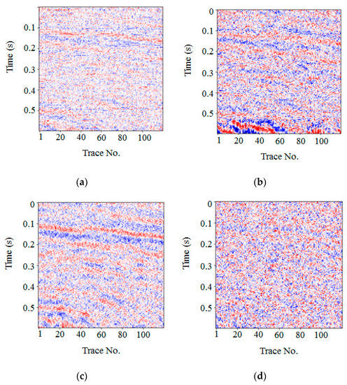
Figure 8.
Comparison of noise removal from synthetic data. The noise was removed using (a) FXDECON, (b) MSSA, (c) wavelet transform, and (d) the proposed method.
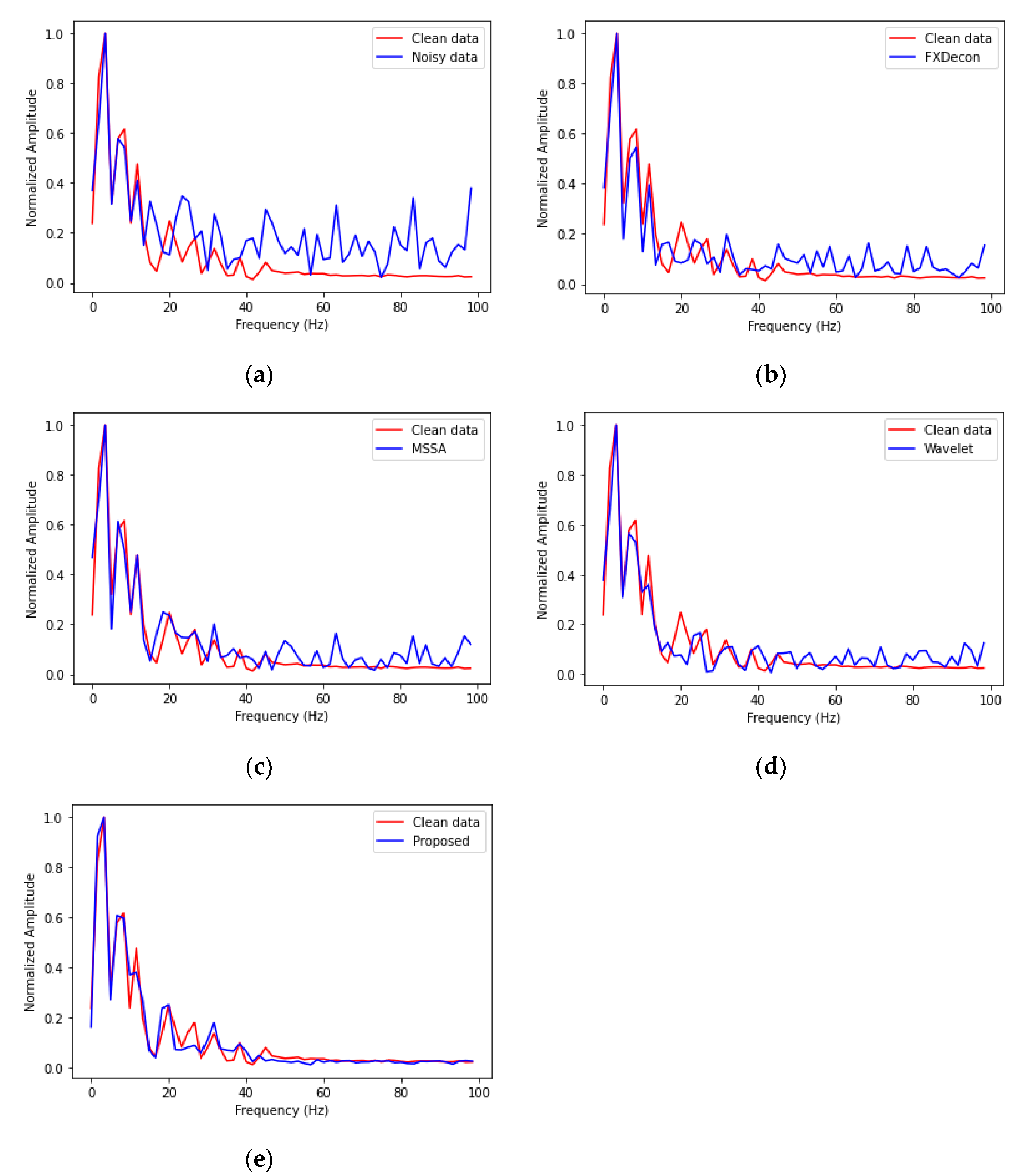
To further study the denoising performance of the four methods, we extracted the 100th channel from the denoising result of the clean data, noise data, FXDON, MSSA, wavelet transform, and the proposed method and calculated the frequency amplitude spectrum, as shown in Figure 9a–d. As shown in the figure, the noise significantly interferes with the effective signal, especially after 40 Hz, which deviates greatly from the effective signal. Moreover, Figure 9b–d shows that the four methods maintain the general shape of the original signal amplitude spectrum within a 0–40 Hz range. After 40 Hz, some random noise was compressed in (b)–(c), but more random noise remained. As indicated in Figure 9d, the sharp peaks in the noise spectrum of the curve were effectively removed, which demonstrated that the proposed method accurately extracted the underlying useful signals from the noisy input.

Figure 9.
Frequency amplitude diagram. (a) Noise and clean signal comparison. (b) FXDECON and clean signal comparison. (c) MSSA and clean signal comparison. (d) Wavelet and clean signal comparison. (e) The proposed method and clean signal comparison. The frequency amplitude spectrum curve of the original signal is indicated in red, whereas the frequency amplitude curve of the denoising result is indicated in blue.
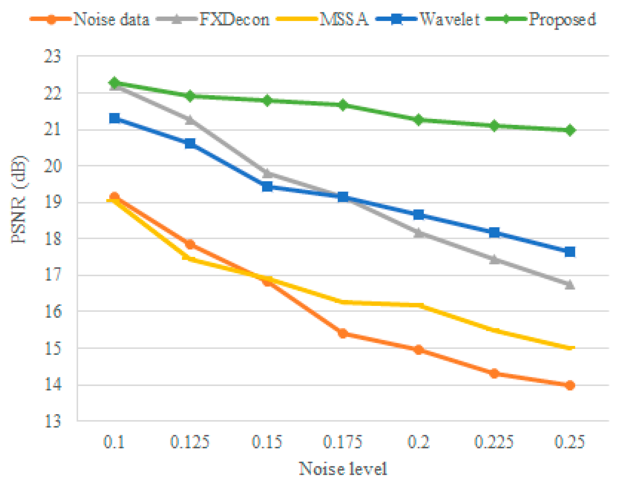
To conduct a more detailed numerical comparison, we selected seven synthetic datasets and added random noise levels of 0.1, 0.125, 0.15, 0.175, 0.20, 0.22.5, and 0.25 based on the normalized data. Figure 10 shows the PSNR noise values of FXDECON, MSSA, wavelet transform, and the proposed method at different random noise levels. As illustrated in the figure, the denoising results of the proposed method were better than those obtained using other methods, demonstrating the excellent denoising performance of the proposed method at different noise levels.

Figure 10.
Denoising PSNR values at different random noise levels. The red line represents the PSNR of the noise signal, and the grey, yellow, blue, and green lines represent the PSNR denoising results by FXDECON, MSSA, wavelet transform, and the proposed method, respectively.
3.2. Application to Real Seismic Signals
To study the denoising performance of the proposed method in practical applications, we analyzed real seismic profile data from the South China Sea. The real profile data had 1000 traces, with a total time of 2 s and a sampling interval time of 2 ms. The frequency range was between 5 and 70 Hz, the wavelength was 300m, and the distance between two traces was 25 m.
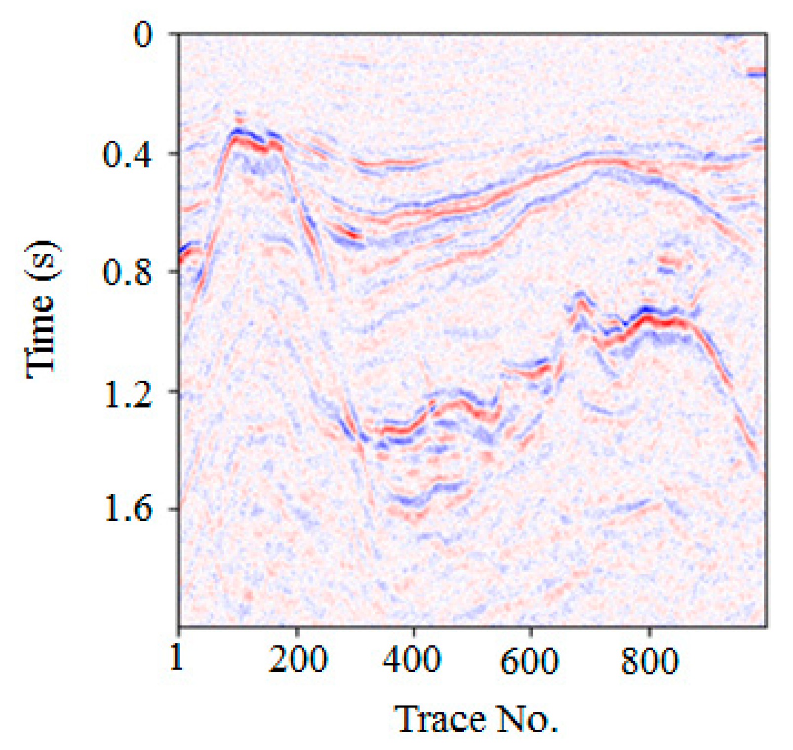
There were several differences between the real and synthetic datasets in our experiments. Table 6 shows a quantitative comparison between the real and synthetic datasets in our experiments. First, the real dataset contained more complicated events that the forward modeling could not achieve, such as more faults, fractures, and buried hills, as observed in Figure 11. Second, the signals of the real data had wide-frequency range characteristics, which meant that more detailed signals were submerged by the noise. Third, we added white Gaussian random noise to the synthetic raw data and obtained the noisy data. However, incoherent background noise mixed with real dataset signals was unstructured, untrackable, and not Gaussian distributed. All these differences presented additional challenges.

Table 6.
Quantitative comparison of the real and synthetic datasets in our experiments.
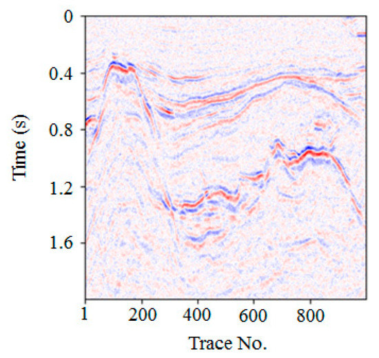
Figure 11.
Real seismic data.
We first randomly collected 43,000 32 × 32 patches in the target region to establish the training set. To verify the denoising effect, we intercepted the test data of 1000 seismic traces and 1000 time samples in the target work area, as shown in Figure 11. Our method was then used to process the real seismic signal. The network structure was the same as described above, including seven convolution layers and other network parameters. The optimized network model was obtained after 25 training epochs, after which it was used to denoise the test seismic signal.
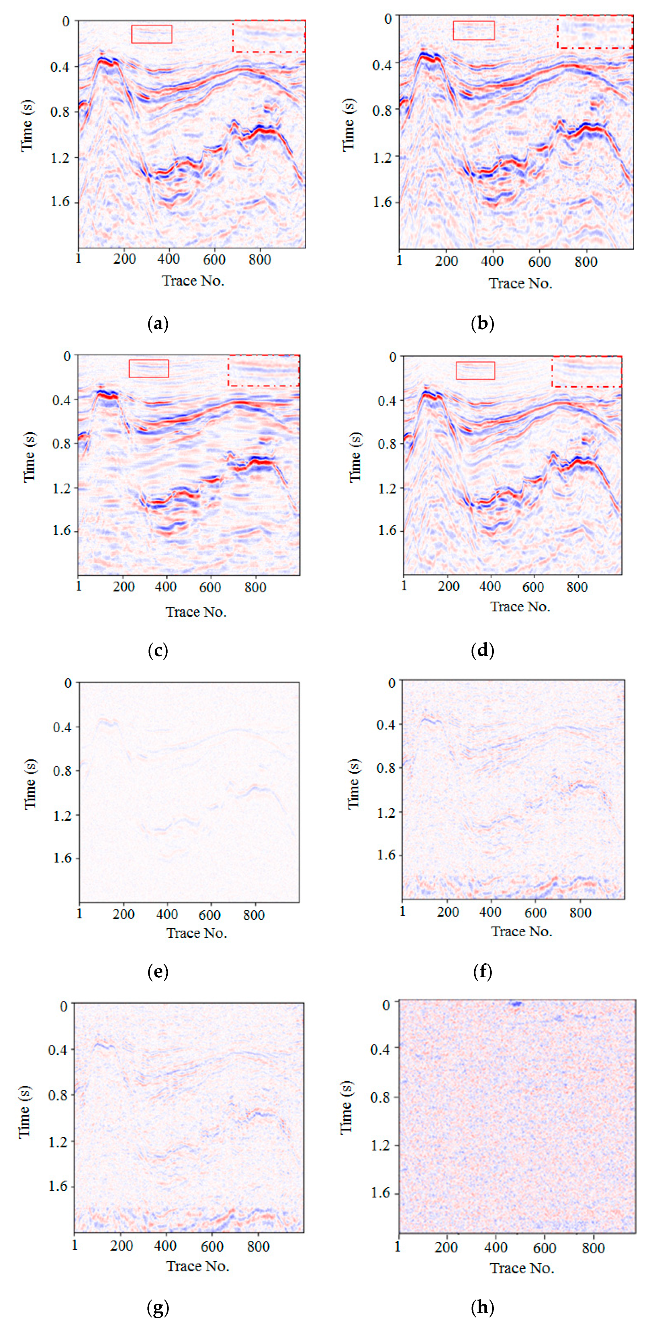
Figure 12a–d showed the denoising results obtained using FXDECON, MSSA, wavelet transform, and the proposed method, respectively. Notably, FXDECON denoising resulted in more residual noise. Moreover, denoising using MSSA and wavelet transform resulted in less residual noise; however, the edge of the event was fuzzy, thereby indicating low fidelity. In contrast, the proposed method rendered less residual noise and clearer signal details. As highlighted in the local correlation map, Figure 12d exhibited more detailed thin-bed reflections and less random noise. However, in Figure 12a,b, the thin-bed details were hazy and difficult to recognise.
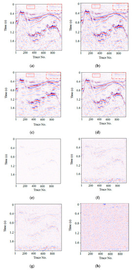
Figure 12.
Denoising comparison of real seismic data results. Denoised results obtained using (a) FXDECON, (b) MSSA, (c) wavelet transform, and (d) the proposed method. Noise removal using (e) FXDECON, (f) MSSA, (g) wavelet transform, and (h) the proposed method.
Figure 12e–h illustrates the noise removal results of FXDECON, MSSA, wavelet transform, and the proposed method, respectively. Among them, the FXDECON, MSSA, and wavelet transform methods left some coherent signals, which indicated that the original signal was damaged during denoising. Moreover, no evident line reflection signal was obtained using the proposed method, which indicated that the proposed method caused no serious damage to the signal during the denoising process. In summary, the denoising performance of the proposed method was better than the others.
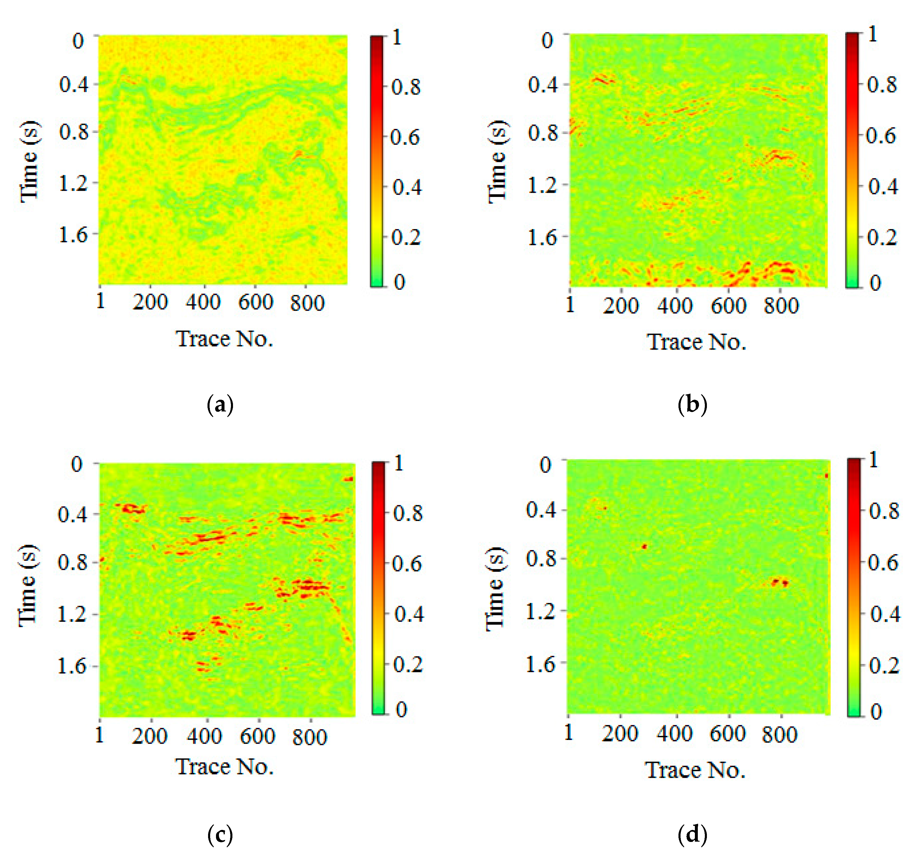
Local similarity describes the similarity of a seismic signal in relation to another one. Therefore, in local similarity analysis, we calculated the local similarity between the denoised result and removed noise to further study the signal leakage of denoised data. Figure 13a–d showed the local similarity analysis between the removed noise and denoising results obtained via FXDECON, MSSA, wavelet transform, and the proposed method, respectively. Local abnormal area similarities indicated that the noise and denoising results of the corresponding position were similar. In turn, this was indicative of signal leakage (i.e., damage to the original signal). As illustrated in the figure, there were many high-similarity abnormal regions in the MSSA and wavelet transform algorithm, which indicated considerable signal damage. In contrast, compared with the other methods, the proposed method exhibited less high-similarity outliers, meaning that the proposed procedure not only rendered less signal leakage but also preserved more effective signals after noise removal.
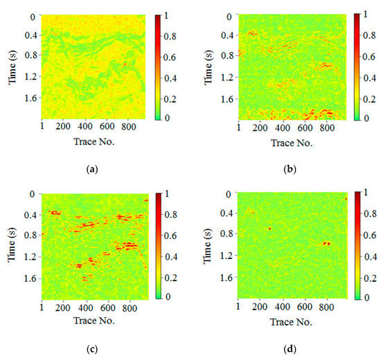
Figure 13.
Local similarity comparison of real data. Local similarity map of (a) FXDECON, (b) MSSA, (c) wavelet transform, and (d) the proposed method.
4. Discussion
In this study, we proposed a tied-weights AE neural network, which presented several advantages. First, our method had a wider scope of application. We directly used patches of raw noise data to establish the training set; therefore, we could prepare the training dataset from the raw data from any real seismic data input. Second, the proposed method benefited from the end-to-end deep convolutional DAE framework and showed a strong ability to extract useful features in the real noisy seismic data. Third, our method accelerated the training process and improved the denoising performance, as we proposed a modified AE neural network based on tied weights to reduce the training number of model parameters and reduce the risk of over-fitting.
However, there were some limitations to the proposed approach. First, the training procedure was generally time-consuming and complicated. Through experimental comparison and analysis, optimal training times and results could be obtained with 32×32 patches and more than 30,000 training sets. Due to a large amount of training data and complex network structure, it took a long time to train the network model. In addition, the network lacked scalability to high-dimensional features. The DAE network corrupted the inputs before mapping them into the hidden representation and then reconstructed the original input from its corrupted version, leading to the loss of some high-dimensional features.
5. Conclusions
Our study proposed a framework for a deep denoising convolutional DAE network to suppress seismic random noise. The scheme was based on AE self-supervised learning, which addressed the limitations of supervised learning (i.e., the requirement for data labels). Unlike conventional approaches, we directly used patches of raw noise data to construct the training and test sets instead of using synthetic clean data or denoising results as training labels. We then designed a robust deep CNN that only depends on the input noise dataset to learn hidden features. Then, we implemented tied weights to reduce the risk of over-fitting and accelerate the training process to obtain optimal network parameters. Finally, we employed a strategy to denoise the target signals using the trained CNN network. The final denoising result was obtained after patch recombination and inverse operation. In quantitative experiments, our tied-weights approach reduced the average training time by 19% and improved the average PSNR value to 1.08 dB in contrast to the non-tied-weights approach. The proposed method also had a higher denoising PSNR value than the other novel denoising algorithms. In qualitative experiments, the proposed method rendered less residual noise and clearer signal details and caused less damage to the signal during denoising. Therefore, both the qualitative and quantitative results demonstrated that the proposed procedure provides a promising means for accurate geological exploration.
Author Contributions
Conceptualization, K.G. and H.Z.; methodology, Y.G. and H.Z.; software, Y.G.; validation, H.Z.; formal analysis, Y.G.; investigation, Y.G.; resources, H.Z.; data curation, H.Z.; writing—original draft preparation, Y.G.; writing—review and editing, H.Z.; visualisation, Y.G.; supervision, H.Z.; project administration, H.Z.; funding acquisition, H.Z. All authors have read and agreed to the published version of the manuscript.
Funding
This research was funded by the Key R&D projects of the Sichuan Science and Technology Department of China (No. 21ZDYF2939).
Data Availability Statement
The data discussed in this paper will be shared on reasonable request to the corresponding author.
Acknowledgments
We would also like to express our gratitude to the Geomathematics Key Laboratory of Sichuan Province and the Key Lab of Earth Exploration and Information Techniques of the Ministry of Education.
Conflicts of Interest
The authors declare no conflict of interest.
References
- Kazemi, N.; Bongajum, E.; Sacchi, M.D. Surface-consistent sparse multichannel blind deconvolution of seismic signals. IEEE Trans. Geosci. Remote. Sens. 2016, 54, 3200–3207. [Google Scholar] [CrossRef]
- Wu, X. Structure—Stratigraphy-and fault-guided regularization in geophysical inversion. Geophys. J. Int. 2017, 210, 184–195. [Google Scholar] [CrossRef] [Green Version]
- Li, F.; Verma, S.; Zhou, H.; Zhao, T.; Marfurt, K.J. Seismic attenuation attributes with applications on conventional and unconventional reservoirs. Interpretation 2016, 4, SB63–SB77. [Google Scholar] [CrossRef] [Green Version]
- Huang, W.; Wang, R.; Li, H.; Chen, Y. Unveiling the signals from extremely noisy microseismic data for high-resolution hy-draulic fracturing monitoring. Sci. Rep. 2017, 7, 11996. [Google Scholar] [CrossRef] [PubMed] [Green Version]
- Zu, S.; Zhou, H.; Mao, W.; Zhang, D.; Li, C.; Pan, X.; Chen, Y. Iterative deblending of simultaneous-source data using a co-herency-pass shaping operator. Geophys. J. Int. 2017, 211, 541–557. [Google Scholar] [CrossRef]
- Dagnino, D.; Sallares, V.; Ranero, C. Waveform-preserving processing flow of multichannel seismic reflection data for adjoint-state full-waveform inversion of ocean thermohaline structure. IEEE Trans. Geosci. Remote. Sens. 2017, 56, 1615–1625. [Google Scholar] [CrossRef]
- Sanchis, C.; Hanssen, A. Multiple-input adaptive seismic noise canceller for the attenuation of nonstationary coherent noise. Geophysics 2011, 76, V139–V150. [Google Scholar] [CrossRef]
- Chen, Y.; Fomel, S. Random Noise Attenuation Using Local Signal and Noise Orthogonalization. In Proceedings of the 77th EAGE Conference and Exhibition, Madrid, Spain, 1–4 June 2015; Volume 80, pp. 1–9. [Google Scholar] [CrossRef]
- Zhou, Y.; Li, S.; Zhang, D.; Chen, Y. Seismic noise attenuation using an online subspace tracking algorithm. Geophys. J. Int. 2017, 212, 1072–1097. [Google Scholar] [CrossRef] [Green Version]
- Liu, G.; Fomel, S.; Jin, L.; Chen, X. Stacking seismic data using local correlation. Geophysics 2009, 74, V43–V48. [Google Scholar] [CrossRef]
- Yang, W.; Wang, R.; Wu, J.; Chen, Y.; Gan, S.; Zhong, W. An efficient and effective common reflection surface stacking approach using local similarity and plane-wave flattening. J. Appl. Geophys. 2015, 117, 67–72. [Google Scholar] [CrossRef]
- Canales, L.L. Random noise reduction. In SEG Technical Program Expanded Abstracts 1984; Society of Exploration Geophysicists: Houston, TX, USA, 1984; Volume 3, pp. 525–527. [Google Scholar]
- Gulunay, N. FXDECON and complex wiener prediction filter. In SEG Technical Program Expanded Abstracts 1984; Society of Exploration Geophysicists: Houston, TX, USA, 1986; pp. 279–281. [Google Scholar] [CrossRef]
- Liu, G.; Chen, X.; Du, J.; Wu, K. Random noise attenuation using f-x regularized nonstationary autoregression. In Proceedings of the International Geophysical Conference, Shenzhen, China, 7–10 November 2011; Volume 77, pp. 61–69. [Google Scholar] [CrossRef]
- Abma, R.; Laerbout, J. Lateral prediction for noise attenuation by t-x and f-x techniques. Geophysics 1995, 60, 1887–1896. [Google Scholar] [CrossRef] [Green Version]
- Naghizadeh, M. Seismic data interpolation and denoising in the frequency-wavenumber domain. Geophysics 2012, 77, V71–V80. [Google Scholar] [CrossRef]
- Mousavi, S.M.; Langston, C. Adaptive noise estimation and suppression for improving microseismic event detection. J. Appl. Geophys. 2016, 132, 116–124. [Google Scholar] [CrossRef]
- Deighan, A.J.; Watts, D.R. Ground-roll suppression using the wavelet transform. Geophysics 1997, 62, 1896–1903. [Google Scholar] [CrossRef]
- Zhang, R.; Ulrych, T.J. Physical wavelet frame denoising. Geophysics 2003, 68, 225–231. [Google Scholar] [CrossRef]
- Ibrahim, A.; Sacchi, M.D. Simultaneous source separation using a robust Radon transform. SEG Tech. Program Expand. Abstr. 2013, 79, 1–11. [Google Scholar] [CrossRef]
- Candès, E.; Demanet, L.; Donoho, D.; Ying, X. Fast discrete curvelet transforms. Multiscale Modeling Simul. 2006, 5, 861–899. [Google Scholar] [CrossRef]
- Herrmann, F.; Böniger, U.; Verschuur, D.J. Non-linear primary-multiple separation with directional curvelet frames. Geophys. J. Int. 2007, 170, 781–799. [Google Scholar] [CrossRef] [Green Version]
- Wang, B.; Wu, R.-S.; Li, J. Simultaneous seismic datainterpolation and denoising with a new adaptive method based on dreamlet transform. Geophysics 2015, 201, 1180–1192. [Google Scholar]
- Fomel, S.; Liu, Y. Jilin University Seislet transform and seislet frame: Tools for compressive representation of seismic data. In Proceedings of the 73rd EAGE Conference and Exhibition—Workshops, Vienna, Austria, 22–27 June 2011; Volume 75, pp. 25–38. [Google Scholar] [CrossRef] [Green Version]
- Chen, Y.; Fomel, S. EMD-seislet transform. SEG Tech. Program Expand. Abstr. 2015, 83, 27–32. [Google Scholar] [CrossRef]
- Oropeza, V.; Sacchi, M. Simultaneous seismic data denoising and reconstruction via multichannel singular spectrum analysis. Geophysics 2011, 76, V25–V32. [Google Scholar] [CrossRef]
- Huang, W.; Wang, R.; Chen, Y.; Li, H.; Gan, S. Damped multichannel singular spectrum analysis for 3D random noise attenuation. Geophysics 2016, 81, 261–270. [Google Scholar] [CrossRef]
- Xue, Y.; Chang, F.; Zhang, D.; Chen, Y. Simultaneous sources separation via an iterative rank-increasing method. IEEE Geosci. Remote. Sens. Lett. 2016, 13, 1915–1919. [Google Scholar] [CrossRef]
- Wu, J.; Bai, M. Incoherent dictionary learning for reducing cross talk noise in least-squares reverse time migration. Comput. Geosci. 2018, 114, 11–21. [Google Scholar] [CrossRef]
- Zu, S.; Zhou, H.; Wu, R.; Mao, W.; Chen, Y. Hybrid-sparsityconstrained dictionary learning for iterative deblending of ex-tremelynoisy simultaneous-source data. IEEE Trans. Geosci. Remote Sens. 2018, 57, 2249–2262. [Google Scholar] [CrossRef]
- Michael, E.; Michal, A. Image denoising via sparse and redundant representations over learned dictionaries. IEEE Tip. 2006, 15, 3736–3745. [Google Scholar]
- Wang, Y.; Zhou, H.; Zu, S.; Mao, W.; Chen, Y. Three-operator proximal splitting scheme for 3-D seismic data reconstruction. IEEE Geosci. Remote. Sens. Lett. 2017, 14, 1830–1834. [Google Scholar] [CrossRef]
- Lecun, Y.; Bengio, Y.; Hinton, G. Deep learning. Nature 2015, 521, 436–444. [Google Scholar] [CrossRef]
- Goodfellow, I.; Bengio, Y.; Courville, A. Deep Learning; MIT Press: Cambridge, MA, USA, 2016. [Google Scholar]
- Liu, D.; Wang, W.; Chen, W.; Wang, X.; Zhou, Y.; Shi, Z. Random-noise suppression in seismic data: What can deep learning do? In SEG Technical Program Expanded Abstracts 2018; Society of Exploration Geophysicists: Houston, TX, USA, 2018; pp. 2016–2020. [Google Scholar]
- Si, X.; Yuan, Y. Random noise attenuation based on residual learning of deep convolutional neural network. In SEG Technical Program Expanded Abstracts 2018; Society of Exploration Geophysicists: Houston, TX, USA, 2018. [Google Scholar]
- Zhang, K.; Zuo, W.; Chen, Y.; Meng, D.; Zhang, L. Beyond a gaussian denoiser: Residual learning of deep CNNs for image denoising. IEEE Trans. Image Process. 2017, 26, 3142–3155. [Google Scholar] [CrossRef] [PubMed] [Green Version]
- Gondara, L. Medical Image Denoising Using Convolutional Denoising Autoencoders. In Proceedings of the 2016 IEEE 16th International Conference on Data Mining Workshops (ICDMW), IEEE, Barcelona, Spain, 12–15 December 2016; pp. 241–246. [Google Scholar]
- Zhang, Y.; Lin, H.; Li, Y. Noise attenuation for seismic image using a deep-residual learning. In SEG Technical Program Expanded Abstracts 1984; Society of Exploration Geophysicists: Houston, TX, USA, 2018; pp. 2176–2180. [Google Scholar] [CrossRef]
- Yu, S.; Ma, J. Deep learning for denoising. In Proceedings of the International Geophysical Conference, Beijing, China, 24–27 April 2018; Volume 84, pp. 1–34. [Google Scholar] [CrossRef]
- Liu, W.; Wang, Z.; Liu, X.; Zeng, N.; Liu, Y.; Alsaadi, F.E. A surveyof deep neural network architectures and their applications. Neurocomputing 2017, 234, 11–26. [Google Scholar] [CrossRef]
- Hall, M.; Hall, B. Distributed collaborative prediction: Results of the machine learning contest. Geophysics 2017, 36, 267–269. [Google Scholar] [CrossRef]
- Huang, L.; Dong, X.; Clee, T.E. A scalable deep learning platform for identifying geologic features from seismic attributes. Lead. Edge 2017, 36, 249–256. [Google Scholar] [CrossRef]
- Chen, Y.; Zhang, M.; Bai, M.; Chen, W. Improving the signal-to-noise ratio of seismological datasets by unsupervised machine learning. Seism. Res. Lett. 2019, 90, 1552–1564. [Google Scholar] [CrossRef]
- Hinton, G.; Zemel, R.S. Autoencoders, minimum description lengthand helmholtz free energy. In Proceedings of the 6th International Conference on Neural Information Processing Systems, Denver, CO, USA, 28 November 28–1 December 1994; Volume 6, pp. 3–10. [Google Scholar]
- Vincent, P.; LaRochelle, H.; Bengio, Y.; Manzagol, P.-A. Extracting and composing robust features with denoising autoencoders. In Proceedings of the 25th International Conference on World Wide Web, Montreal, QC, Canada, 11–15 April 2016; pp. 1096–1103. [Google Scholar]
- Vincent, P.; Larochelle, H.; Lajoie, I.; Bengio, Y.; Manzagol, P.-A. Stacked denoising autoencoders: Learning useful represen-tations in a deep network with a local denoising criterion. J. Mach. Learn. Res. 2010, 11, 3371–3408. [Google Scholar]
- Alain, G.; Bengio, Y. What regularized auto-encoders learn from the data-generating distribution. J. Mach. Learn. Res. 2012, 15, 3563–3593. [Google Scholar]
- Deng, J.; Zhang, Z.; Eyben, F.; Schuller, B. Autoencoder-based unsupervised domain adaptation for speech emotion recognition. IEEE Signal Process. Lett. 2014, 21, 1068–1072. [Google Scholar] [CrossRef]
- Donahue, J.; Jia, Y.; Vinyals, O.; Hoffman, J.; Zhang, N.; Tzeng, E.; Darrell Decaf, T. A deep convolutional activation feature for generic visual recognition. In Proceedings of the International Conference on Machine Learning, Beijing, China, 21–26 June 2014; pp. 647–655. [Google Scholar]
- Wang, S.; Li, Y.; Zhao, Y. Desert seismic noise suppression based on multimodal residual convolutional neural network. Acta Geophys. 2020, 68, 389–401. [Google Scholar] [CrossRef]
- Sun, J.; Slang, S.; Elboth, T.; Greiner, T.L.; McDonald, S.; Gelius, L.-J. A convolutional neural network approach to deblending seismic data. Geophysics 2020, 85, WA13–WA26. [Google Scholar] [CrossRef]
- Vincent, P.; Larochelle, H.; Bengio, Y.; Manzagol, P.A. Extractingand composing robust features with denoising autoencoders. In Proceedings of the 25th International Conference on Machine Learning (ICML 2008), Helsinki, Finland, 5–9 July 2008; pp. 1096–1103. [Google Scholar]
- Liou, C.-Y.; Huang, J.-C.; Yang, W.-C. Modeling word perception using the Elman network. Neurocomputing 2008, 71, 3150–3157. [Google Scholar] [CrossRef]
- Santurkar, S.; Tsipras, D.; Ilyas, A.; Madry, A. How does batch normalization help optimization? In Proceedings of the 32nd International Conference on Neural Information Processing Systems, Montréal, QC, Canada, 3–8 December 2018; Curran Associates Inc.: Red Hook, NY, USA, 2018; pp. 2488–2498. [Google Scholar]
Publisher’s Note: MDPI stays neutral with regard to jurisdictional claims in published maps and institutional affiliations. |
© 2021 by the authors. Licensee MDPI, Basel, Switzerland. This article is an open access article distributed under the terms and conditions of the Creative Commons Attribution (CC BY) license (https://creativecommons.org/licenses/by/4.0/).


