Article

Prediction of Uniaxial Compression Strength of Limestone Based on the Point Load Strength and SVM Model

1
School of Resources and Safety Engineering, Central South University, Changsha 410083, China
2
School of Civil Engineering, Beijing Jiaotong University, Beijing 100044, China
*
Authors to whom correspondence should be addressed.
Minerals 2021, 11(12), 1387; https://doi.org/10.3390/min11121387
Submission received: 15 November 2021 / Revised: 4 December 2021 / Accepted: 6 December 2021 / Published: 8 December 2021

Abstract

:
Uniaxial compression strength (UCS) is a fundamental parameter to carry out geotechnical engineering design and construction. It is simple and efficient to predict UCS using point load strength (PLS) at engineering sites. However, the high dispersion of rock strength limits the accuracy of traditional fitting prediction methods. In order to improve the UCS prediction accuracy, 30 sets of regular cylindrical specimen tests between PLS and UCS are conducted on limestone mines. The correlation relationship between PLS and UCS is found by using four basic fitting functions. Then, a prediction model is established by using SVM algorithm. Multiple training test data are used to achieve high-precision prediction of UCS and the results show it is less different from the actual values. Especially, the R2 coefficient reached 0.98. The SVM model prediction performance is significantly better than the traditional fitting function. The constructed SVM model in this study can accurately predict the UCS using the PLS obtained in the field, which has a great significance to the rock stability judgment in the actual construction environment.

1. Introduction

Construction projects such as water and hydropower, transportation, mining, industrial and civil construction engineering all involve rock engineering. In order to accurately and promptly assess the stability of the mountains involved in the construction project and ensure the safety of the structure, rock classification methods are often used in the rock engineering project and design. To evaluate the stability of engineering rock mass, the rock classification divides engineering rock mass into several levels with different basic quality and strength. In this way, it provides an important basis and safety protection selection for the technical planning and various construction engineering [1].
Quantitative indicators of strength in rock classification are generally expressed in terms of uniaxial compression strength of rocks. However, the determination of the uniaxial compression strength usually needs to be measured in the laboratory, which cannot meet the requirements of obtaining data quickly at the engineering site [2]. In 1972, Broch and Franklin [3] gave the first point load strength formula by studying the damage model analysis of cylindrical specimens analyzed along the diameter direction and found that the uniaxial compression strength values of certain rocks were approximately 24 times higher than those of rock specimens tested with a 50 mm diameter point load. This discovery provided an alternative method of simple operation and high accuracy for testing the uniaxial compression strength on the engineering site. Compared with the uniaxial compression strength, testing the point load strength of the rock has the advantages of convenience and efficiency, and the strength index of the rock can be obtained in a shorter time period. This makes the point load strength very important in engineering practice. It is widely used in practical scenarios such as tunnel engineering, slope stability analysis, mining roadway support, etc [4,5]. Subsequently, many scholars and scientific research institutions have launched a large number of related research.
Bieniawski [6] stated that the uniaxial compression strength of rocks is about 23 times the point load strength. The International Society of Rock Mechanics [7] and the American Society for Testing Materials [8] proposed a general test method and procedure for point load strength and gave a general formula R = (20~25) Is(50) between them in 1985. Tsiambaos and Sabatakakis [9] studied the ratio of uniaxial compression strength to point load strength for intact sedimentary rocks. The test results showed that this ratio varied with different point load strength distributions. For example, different ratios existed from soft sedimentary rocks with point load strength less than 2 MPa to hard rocks with point load strength more than 5 MPa. A. Basu and M. Kamran [10] have explored the feasibility of point load tests to evaluate anisotropic rocks uniaxial compression strength such as schists based on successful estimation of uniaxial compression strength by point load tests on isotropic rocks. Through evaluating uniaxial compression strength of these rocks, relevant fitting formulas have been obtained with good prediction results. Robina H. C. Wong [11] investigated the correlation between point load strength and uniaxial compression strength of irregular volcanic rock masses from 16 different locations and obtained a good linear fit based on the analysis of all test data. Accordingly, they found a suitable size correction factor by least squares method.
Based on the summary of a large number of literatures, these research results are arranged in the table by year, as shown in Table 1. It can be identified that many scholars [12,13,14,15,16,17,18,19,20,21,22,23,24,25,26,27] have found the correlation between point load strength and uniaxial compression strength by experimental methods. However, the data processing of these research results is carried out by function fitting, and there are large deviations in predicting the test points that deviate from the data center. Moreover, it can be found from Table 1 that most of the derived correlation formulas are linear, but some of them are nonlinear functions such as exponential, logarithmic, and power functions. These results also imply that there exists a nonlinear relationship of limestone between the point load strength and the uniaxial compression strength [14,26]. This shows that large deviation will be produced if the general linear formulas are simply used to perform the uniaxial compression strength estimation. So linear relationship cannot be blindly extended to all engineering scenarios for undeveloped projects [28,29].
The shortcomings shown above indicate that the currently derived conversion formulas still have large errors for engineering applications, and some of them even fail to meet the engineering accuracy requirements for direct application in actual engineering. In view of this, it is necessary to further study and establish the correlation model between rock uniaxial compression strength and point load strength to improve the prediction accuracy and calculation.
With the continuous progress in computational science, techniques such as machine learning and artificial intelligence, many scholars have applied these to the field of civil and mining engineering to solve many engineering challenges encountered. For example, Yilmaz and Yuksek [16] developed a high-performance adaptive neural network model for predicting gypsum strength and elastic modulus to reduce rock engineering project uncertainty. Ruhul Amin Mozumder [30] used an artificial neural network model to analyze the effect of different geopolymer ratios on uniaxial compression strength and predicted uniaxial compression strength by this model. The usage of these methods improved the prediction model reliability and accuracy to a greater extent and were more accurate in predicting discrete points that deviate from the data center region compared to traditional fitting methods.
Based on these research experiences, a prediction model based on machine learning algorithm can be developed in conjunction with the correlation relationship existing between point load strength and uniaxial compression strength, which can further enhance the prediction accuracy. In this study, 30 groups of corresponding point load tests and uniaxial compression strength tests were conducted, and four basic function types were used to fit and regress the data in order to investigate the correlation relationship between uniaxial compression strength and point load strength. Then a computational model with high accuracy was established for predicting uniaxial compression strength based on support vector machine algorithm. The model can be used to quickly determine the rock strength level at engineering sites, which provides a reference for construction design and safe production.

2. Methods and Materials

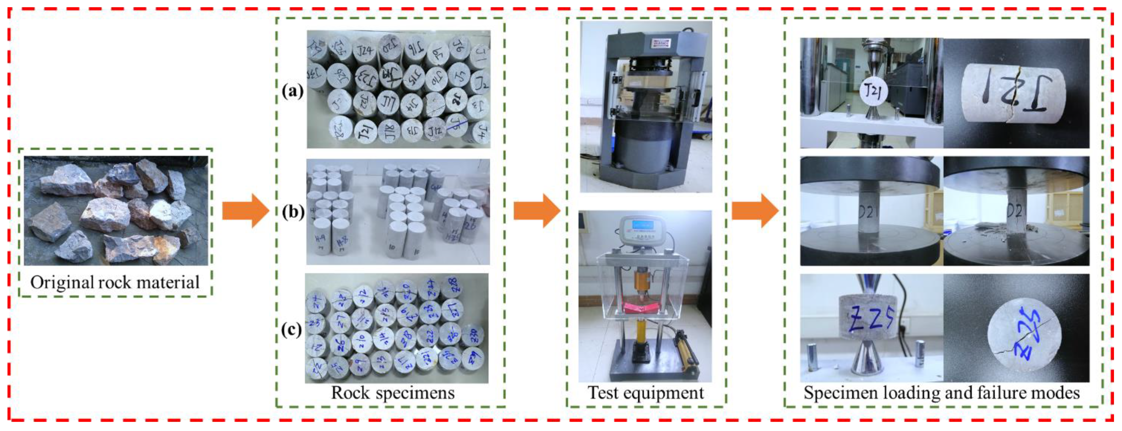
2.1. Rock Sampling and Fabrication

Point load strength tests can be performed on all types of rocks in nature, and test specimens are mainly divided into regular and irregular blocks according to the specimen’s integrity. In general, the use of irregular specimens makes the field operation procedure more convenient, but the accuracy of this method is relatively low, so regular blocks for point load strength parameter determination is more in line with the practical needs [31,32,33]. In order to improve accuracy of the point load strength index, this study uses regular cylindrical specimens for testing and analysis.
As we all know, rock is a kind of non-uniform material, and there are pores and micro cracks in it. These factors will affect the macro mechanical strength of rock such as UCS and PLS [34], so complete specifications and no obvious fissures rocks were selected when collecting. The rock samples in this study were obtained from the limestone mine of Sichuan Red Lion Cement in China. The main component of the rock is calcium carbonate, which locally contains 10%~25% argillaceous limestone sand debris. The main density distribution of limestone in the mine is 2.65~2.83 g/cm3. The nature of the rock is limestone with uniform block size, good integrity and regular shape, which can meet the test requirements. The rock specimens were prepared on this basis.
In order to prepare test specimens, holes were drilled in the collected rocks to obtain initial specimens with a 50 mm diameter, which were marked. About 4 to 6 initial specimens were obtained on a single rock. Subsequently, these initial specimens were cut and polished to produce UCS and PLS rock specimens with smooth and flat surfaces and no obvious fissures. Ultimately, the uniaxial compression strength test specimens were prepared as standard cylindrical specimens with 100 mm height and 50 mm diameter. The point load test specimens were cylindrical in overall shape with 50 mm diameter, the diametral loading specimens’ height was 70 mm, and the axial loading specimen’s height was 30 mm.
The rock specimens and equipment used in the test are shown in Figure 1. In this study, 30 specimens were separately prepared for axially loaded point load test, diametral loaded point load test and uniaxial compression test, totaling 90 rock specimens. The water content of the specimens was natural and the tests were run at room temperature.

2.2. Point Load Strength Test

Point load test applies a concentrated load at the tip of the rock specimen until the specimen is destroyed, and the point load strength of the specimen can be obtained by calculation. The larger the concentrated load on the specimen, the greater the point load strength obtained. The concentrated loading methods mainly include diametral and axial, from which the diametral point load strength (DPLS) and axial point load strengths (APLS) are obtained, both of which have comparable reliability and same applied [35,36].
The test method procedure in common use today is mainly the recommended method for point load strength testing proposed by the International Society of Rock Mechanics in 1985. The ISRM method uses the concept of equivalent diameter De to calculate the point load strength. Moreover, to make the resultant data more comparable, the calculated raw Is is generally converted to the point load strength Is(50) at De = 50 mm as follows:
I s = P D e 2
In Formula (1), P represents the point load, De is the equivalent core diameter (mm).
I s ( 50 ) = F I s
In Formula (2), F represents the correction factor.
F = ( D e 50 ) m
In Formula (3), m is the correction index, generally desirable 0.40~0.45, or according to the value of similar rocks to determine the experience.
In this study, point load strength tests were respectively conducted using both diametral loading and axial loading. When the diametral test was used, the equivalent core diameter was calculated according to the following equation:
D e 2 = D 2
In Formula (4), D is the loading point spacing (mm). When the axial test is used, the equivalent core diameter is calculated according to Formula (5):
D e 2 = 4 W D π
In Formula (5), W is the width or the smallest section average width through the two loading points (mm).
The test procedure was carried out according to ISRM. During the test, specimens were placed between the upper and lower loading cone heads of the point load strength tester, and the lower cone head was raised by cranking the hand crank oil pump to maintain the loading speed between 0.05~0.1 MPa. The damage occurred within 10~60 s. The rock specimen is damaged between the two loading heads, forming a damage surface through the upper and lower loading points. A typical damage diagram is shown in Figure 1.

2.3. Uniaxial Compression Strength Test

Uniaxial compression strength is the main index to evaluate rock stability and rock classification. Put the rock sample between the upper and lower pressing plates of the press. When the sample is crushed, its pressure strength value can be measured, which is the uniaxial compression strength. The greater pressure the rock can bear, the higher the uniaxial compression strength is [37].
Uniaxial compression strength test also refers to the ISRM standard. A total of 30 Rock standard specimens are used in the test. The specimens are tested on the HCT-206A rock true triaxial compression testing machine (Figure 1) and loaded to failure at the speed of 0.6 MPa/s. The ultimate stress value on the compression surface at the moment of failure is the uniaxial compression strength of the rock, and the specimens will undergo monotonic failure under axial load. The uniaxial compression strength is calculated according to Formula (6):
R = P A
In Formula (6), R is the uniaxial compression strength of the rock, MPa; P is the peak breaking load, N; A is the initial cross-sectional area of the specimen, mm2.

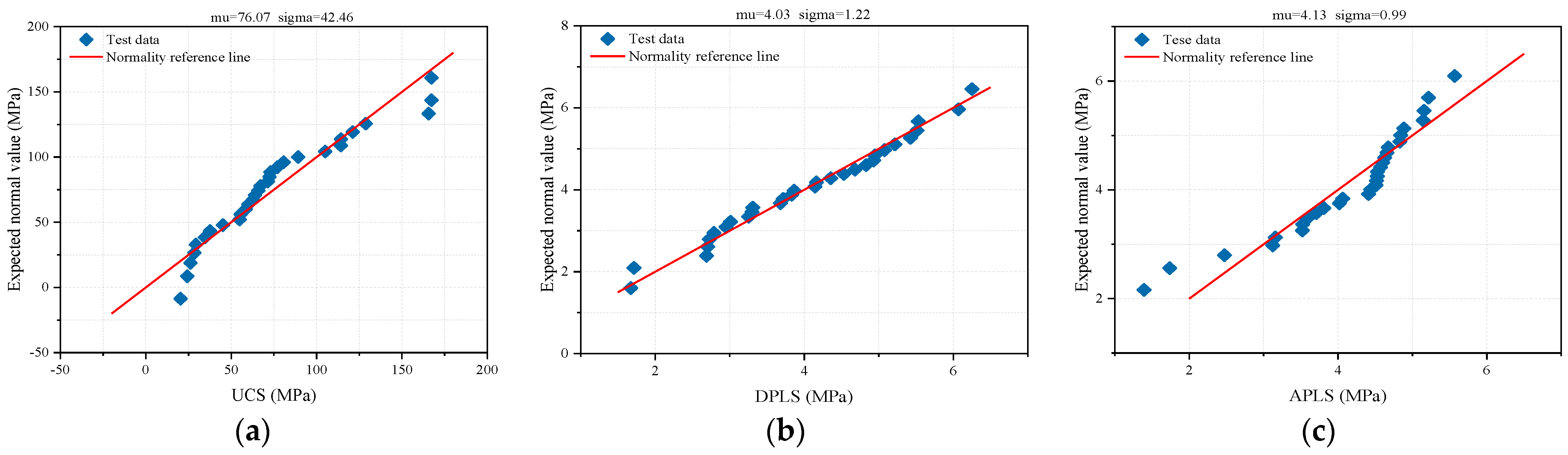
2.4. Data Analysis and Inspection

In the point load strength test and uniaxial compression strength test, data distortions caused by improper test operations often occur. In this study, such apparently abnormal data were eliminated, and Grubbs’ criterion was used to test whether there were suspicious data, and when the suspicious data satisfied Formula (7), they should be eliminated from the group.
| X p X ¯ | > G p ( n ) S
In Formula (7), Xp is the data being tested, X ¯ is the average value, S is the standard deviation, Gp(n) is the test threshold, where p is the confidence probability, taken as 0.95, and n is the number of data, taken as 30.
After rigorous calculations, the Grubbs test value of diametral point load strength data is 1.97, the Grubbs test value of axial loading point load strength data is 2.77, and the Grubbs test value of uniaxial compression strength test data is 2.15, which has no abnormal value at 5% significance level and satisfies the condition of no abnormal value of test data. The above analysis indicates that test data obtained from the experiment has high reliability.

3. Result and Analysis

3.1. Experimental Data Results

After the test according to the scheme, all the test data were measured in this study, which can be obtained from supplementary materials (Table S1–S3). Then, we drew a Q-Q chart to examine the normality of the data, as shown in Figure 2. The data distribution, mean, and standard deviation of the three experiments also can be obtained in Figure 2. It can be found that the UCS average value is 76.07 MPa and standard deviation is 42.46 MPa. The DPLS average value is 4.03 MPa and standard deviation is 1.22 MPa. The APLS average value is 4.13 MPa and standard deviation is 0.99 MPa.
It can be seen from the figure that the three experiments data are in accordance with the normal distribution law within the confidence interval of 95% level. The sample average can well represent the overall data level and data concentration degree [38].

3.2. Discussion and Analysis

Firstly, the relationship between APLS and UCS is found. As shown in Figure 3a, the correlation coefficient by linear fitting is 0.8883, logarithmic fitting is 0.7768, exponential fitting is 0.9485, and power function fitting is 0.9485. Then four relations between the APLS and UCS are obtained, as shown in Figure 3b. The correlation coefficient of linear fitting is 0.6873, logarithmic fitting is 0.5313, exponential fitting is 0.8846, and power function fitting is 0.7680.
From these fitting results, the correlation coefficients using exponential function fitting are greater than other function fitting, whether axial loading or diametral loading, which has better fitting effect, indicating that the relationship between PLS and UCS in this mine is more aptly described in the form of exponential function.
According to the exponential function relationship, the predicted value by using this formula is compared with the experimental value, and the error value is presented in Figure 4. It can be seen from the prediction effect of the final fitting function that even if the exponential function with the largest correlation coefficient is used for strength prediction, the calculation accuracy still deviates too much from the actual requirements, especially in the high-strength rocks. The maximum deviation reached 47.53 MPa, and concentrated in the axial point load strength area. This shows that the traditional fitting method has poor accuracy and cannot adapt to the high dispersion disadvantages of rock strength [39].
Through the above tests and data analysis, it can be known that there is an obvious non-linear relationship between the point load strength of the mine’s limestone and the uniaxial compression strength. On this basis, the artificial intelligence algorithm can be used to construct the relationship model between both. Data training can improve the accuracy of the model to meet engineering needs.

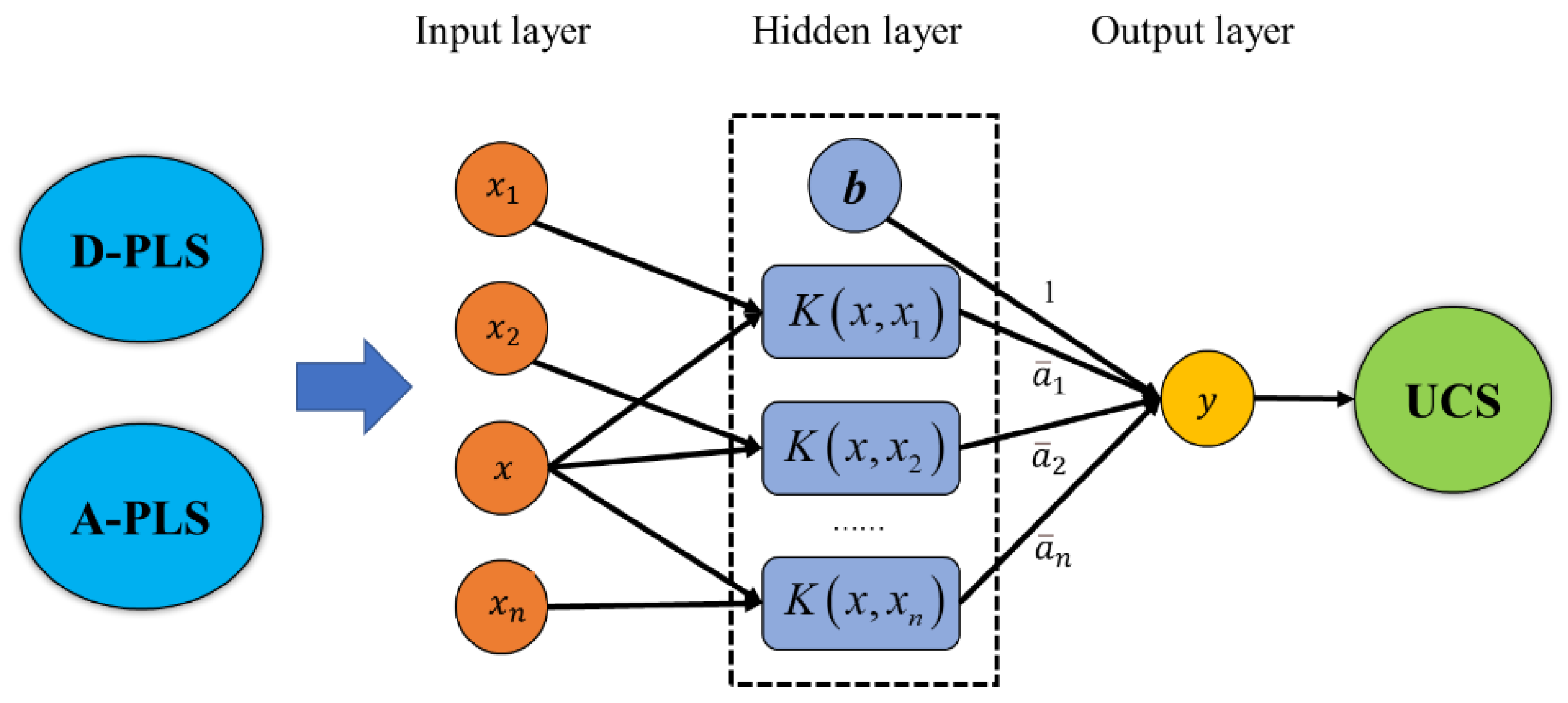
4. Support Vector Machine Model

4.1. Theoretical Basis

Support vector machine (SVM) is a classical artificial intelligence algorithm. SVM model can theoretically approximate any nonlinear function in a global sense. It improves the generalization ability of the model according to the principle of structural risk minimization and can obtain better statistical laws with a small statistical sample size [40]. SVM has the significant advantage of transforming the problem to a high-dimensional feature through nonlinear transformation space, thus avoiding catastrophic data phenomena, local miniaturization, and other problems that often occur in the prediction process [41,42,43].
SVM is a machine learning mechanism. The essence of machine learning is to obtain the relationship estimation between input and output of the system from a given finite sample [44]. Thus, it can make a more accurate prediction of the unknown output. In terms of development, support vector machine theory is developed based on statistical learning theory, which overcomes many shortcomings of classical statistical methods and empirical nonlinear methods [45]. The rock test has the nature of small samples. Each strength index has an obvious non-linear relationship, so it is very suitable to use the SVM model to solve the data prediction problem related to rock specimens. The principle of SVM nonlinear regression is briefly described below [46,47].
For a set of real numbers H = {(xi, yi)}, where i = 1, 2,…, n, it is assumed that the functional relation y = g(x) is fitted between xi and yi, where xi is the input quantity in this relation, yi is the output quantity, and n is the sample capacity. For this functional relationship, the fitted relationship equation used in SVM is:
f ( x ) = ω φ ( x ) + b
In Formula (8), f(x) is the fit function, φ(x) is the nonlinear mapping function, ω is the weight vector, and b is the partiality constant.
Support vector machines use a structural risk minimization strategy by which ω and b can be obtained:
S m = C i = 1 n L ε ( y i , f ( x i ) ) + 1 2 ω 2
In Formula (9), L ε ( y i , f ( x i ) ) is the empirical risk function, 1/2 ω 2 is the regularization term, C is the penalty coefficient, and Lε is the insensitive loss function of ε.
Sm can prevent the decision function from over-fitting, and then continue to introduce slack variables ξ i and ξ i * , so that the minimization of Sm is abbreviated as:
min S m = 1 2 ω 2 + C i = 1 n ( ξ i + ξ i * )
Subject   to   { y i b [ ω ϕ ( x i ) ] ε + ξ i [ ω ϕ ( x i ) ] + b y i ε + ξ i , ξ i * 0 , i = 1 , , n ξ i *
To determine the range of ω, the solution is performed by Lagrange optimization method, which leads to:
ω = i = 1 n ( a i a i * ) ϕ ( x i )
In Formula (12), a i and a i * are Lagrange multipliers corresponding to sample of i.
The final decision function is obtained by substituting Formula (12) into Formula (8):
f ( x ) = i = 1 n ( a i a i * ) K ( x , x i ) + b
K ( x , x i ) = ϕ ( x i ) ϕ ( x k )
After establishing the model, R2 and mean square error (MSE) are used to evaluate the performance of established model. R2 can be used to measure how well the predicted values fit the true values. In the ideal case, the value of R2 is 1. The more R2 converges to 1, the better the prediction performance of the model, which is calculated as in Formula (15):
R 2 = 1 i = 1 n ( U p U i ) i = 1 n ( U i U )
In Formula (15), Up is the predicted value of uniaxial compression strength, Ui is the true value of uniaxial compression strength, U represents the average value of the true uniaxial compression strength of the group of tests, and n is the sample capacity.
The MSE refers to the average value of the difference between the predicted value and the actual value after the sum of the squares. It is often used to measure the prediction model accuracy and evaluate the data change degree. The smaller the value of the MSE, the better the model’s ability to fit experimental data. The calculation formula is as follows:
M S E = 1 n i = 1 n [ U p U i ] 2

4.2. Model and Results

Based on the above theoretical basis, the SVM method is used to establish the relationship model between PLS and UCS. As shown in Figure 5, the model uses APLS and DPLS as input vectors. Kernel function and partiality constant b is used as the hidden layer, and y represents the measured UCS value.
The introduction of the kernel function makes the SVM perfectly solve the problem of sample nonlinearity, so that the inner product operation of the vector in the high-dimensional space is transformed into the function of the vector in the original space, which effectively handles the input of the high-dimensional vector and can directly affect the SVM model performance. At present, the kernel functions commonly used in SVM models include linear kernel function, polynomial kernel function, Gaussian kernel function, Laplacian kernel function, and Sigmoid kernel function. Among them, the Gaussian kernel function has strong learning ability and can be used in the absence of research samples. A good predictive effect is obtained when the prior knowledge is obtained [48]. The SVM constructed in this study uses a Gaussian kernel function, and the specific equation is shown in Formula (17), where γ is the kernel parameter of the kernel function [49]:
K ( x i , x k ) = exp ( γ x i x k 2 )
The SVM is used to establish the uniaxial compression strength prediction model M1, as shown in Figure 6. The input vector currently is the APLS and the corresponding DPLS, and the output vector is the UCS. After sorting out the experimental data, randomly divide 25 groups of data into the training set, and the remaining 5 groups of data into the prediction set. Then run the model.
After a large amount of training with data in the training set, the model accuracy and generalization ability continue to improve. According to the model M1 prediction results, the MSE in the training set is 62.66, R2 reaches 0.96937, the MSE of the prediction set is 50.05, and R2 is 0.98, which shows the SVM model has a high fit degree and a small deviation from the average. It is found that the sample area with UCS lower than 100 MPa has higher prediction accuracy than the sample area with UCS higher than 100 MPa. Compared with some existing studies [9,15,26], the R2 coefficient of model M1 is higher and the prediction performance is better.
According to the practical application experience of SVM model, the main parameters affecting the prediction results are penalty factor C and sensitive parameter γ. By finding the optimal C and γ, the applicability of the model can be optimized. The parameters used in this study are shown in Table 2.
Subsequently, we establish the relationship model M2 for predicting UCS by using DPLS. As shown in Figure 7, the results show that the MSE in the training set is 48.24, R2 is 0.97, the MSE in the prediction set is 76.44, and R2 is 0.99. There is not much difference between the predicted value and the true value in the prediction set.
Under the same grouping conditions, we establish the relationship model M3 to predict UCS by APLS. As shown in Figure 7, the MSE also obtained in training set is 19.81, R2 is 0.98, and the MSE in the prediction set is 176.48, R2 reached 0.96. It can be found that the predicted value of sample No. 4 and sample No. 5 has a large error with the true value. The main reason is that the training data amount is small, and the strength discreteness interferes with the prediction accuracy.
It can be seen from the two model evaluation indexes that the accuracy of model M2 is higher than that of model M3, and the evaluation indexes of the M2 are better. Therefore, for this mining project, it is more suitable to use diametral loading for point load strength test in the field, which can quickly predict the uniaxial compression strength and enhance the efficiency and geotechnical design capability.
Combining the performance results of the three models, the overall performance of model M1 is better and the accuracy is the highest. This shows that the prediction method of using APLS and DPLS to predict UCS is better than using only a single type of point load strength. When the engineering economic conditions permit, the axial point load test and the diametral point load test should be carried out at the same time to obtain the best prediction effect.

4.3. Limitations

The main content of this research is the correlation between the PLS and the UCS, and exploring the feasibility and predictive performance of the SVM model in predicting the uniaxial compressive strength by using the point load strength. Although this model has significant performance and advantages in predicting the uniaxial compressive strength of rocks, it also has some limitations that require deeper research.
  • The mechanical strength of rock has a high degree of dispersion, and the amount of data used in this model is small, which may easily lead to errors in the prediction of the strength of individual specimens [50]. In order to indicate the accuracy and stability of the model, further research is required of more relevant test data sets for verification.
  • This study only focuses on the model relationship between the point load strength and the uniaxial compressive strength. Other indicators involved in the test, such as specimen loading point spacing D and the minimum cross-sectional width W, have not been involved. The specific relationship between other variables and the uniaxial compressive strength of the rock is not clear.
  • In order to better improve the prediction performance and accuracy of the model, it is necessary to better optimize and search the built-in parameters of the established SVM model, such as the penalty factor C and kernel parameter γ. The calculation work in this area can be enhanced in the following research.

5. Conclusions

Through the test results analysis, it was found that the PLS of the limestone in the mine area had an exponential relation with the UCS. Then based on the exponential relationship, the SVM models for predicting UCS by DPLS and APLS are established respectively, and the following conclusions are drawn:
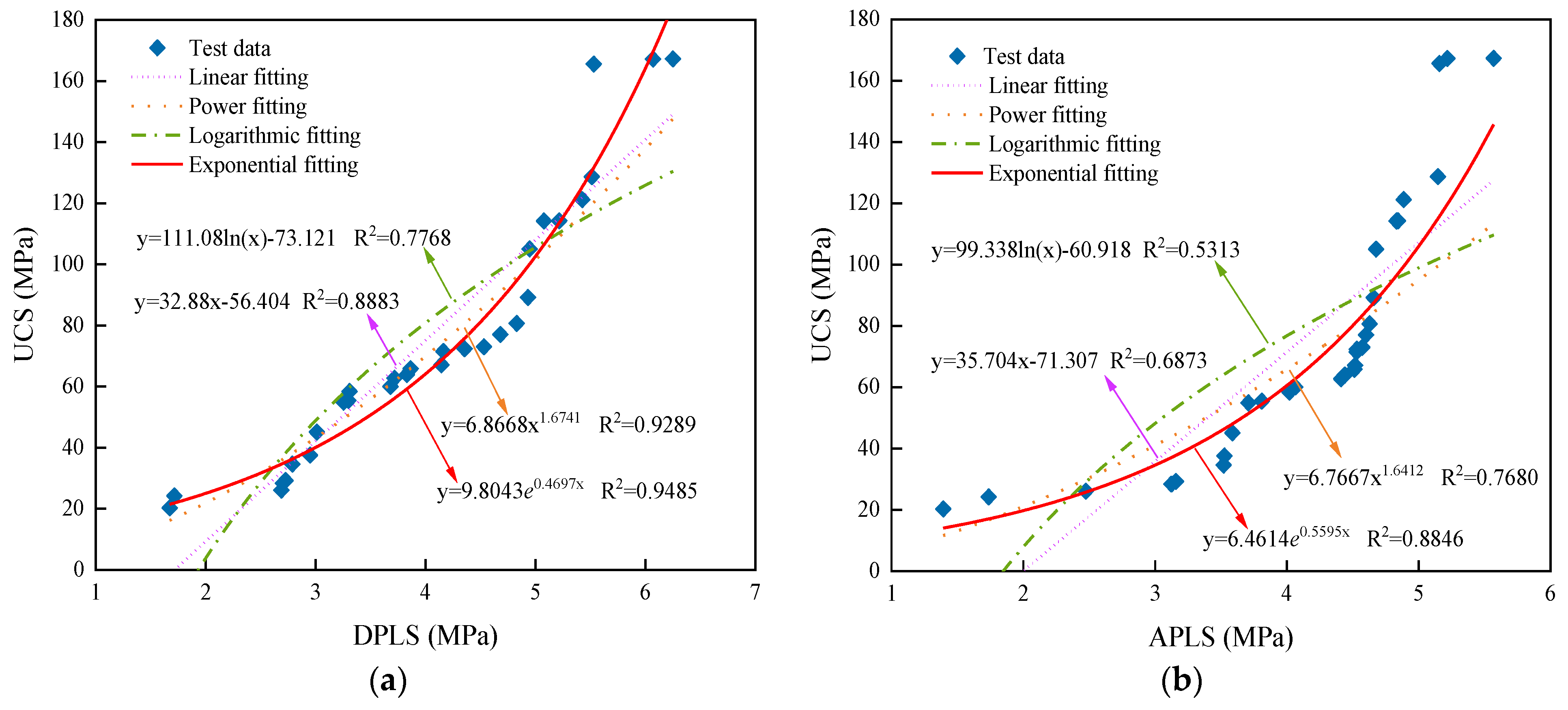
  • Four fitting methods are both used to obtain the formula with the highest correlation coefficient. The most accurate fitting formula and function for APLS and UCS is R = 6.46e0.56Is(50), where R2 is 0.8846, and the most accurate fitting formula for DPLS and UCS is R = 9.80e0.47Is(50), where R2 is 0.9485. The above formulas are all expressed as exponential functions.
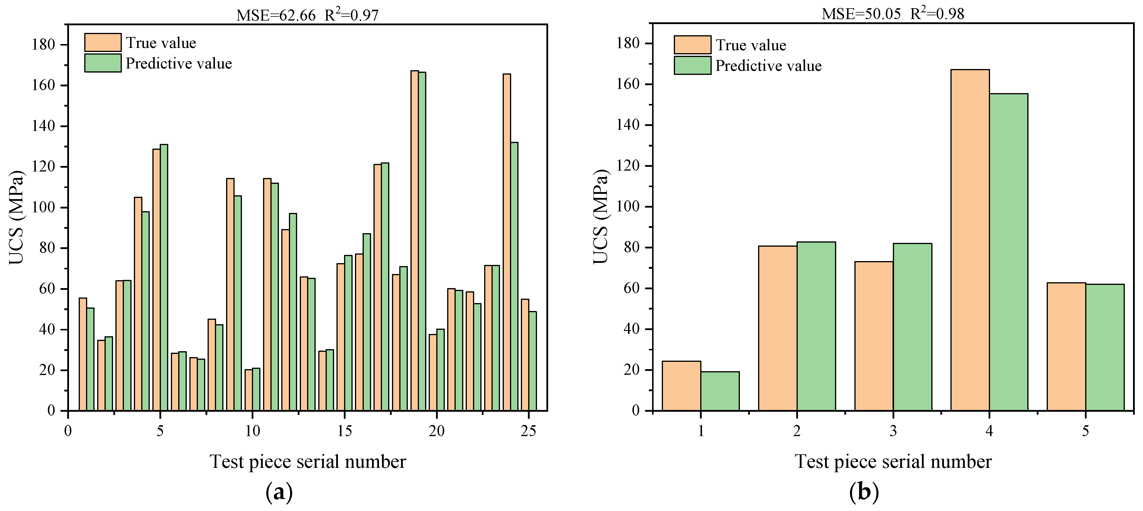
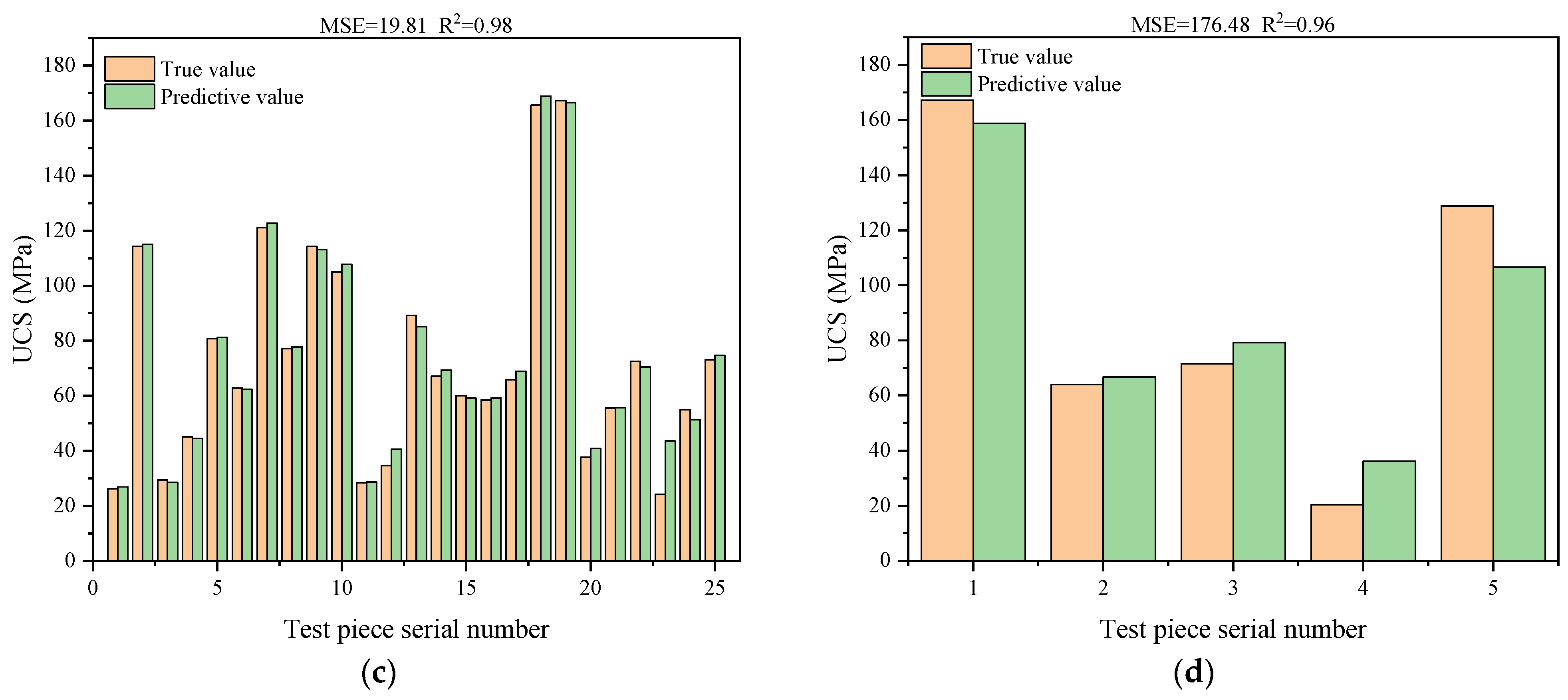
  • The proposed SVR model can accurately predict the UCS through the PLS. The predicted value is basically the same as the true value, and the maximum error rate is below 15%. The SVM model prediction result is more accurate compared with the traditional fitting methods and it also proves that the SVM algorithm can be better applied to the rock strength prediction scenarios under the condition of small samples.
  • For the first time, the APLS and DPLS are both used as an entirety to predict the UCS, and the prediction model M1 was established. By comparing the three models, it is found that in the R2 performance: the correlation coefficient of model M2 is the largest and the correlation coefficient of M3 is the smallest. In the MSE performance, the MSE of model M1 is the smallest and the M3 model is the largest. Combining the R2 and MSE judgment indexes, model M1 has the best overall performance, which indicates that the accuracy of predicting UCS by using APLS together with DPLS is the highest.
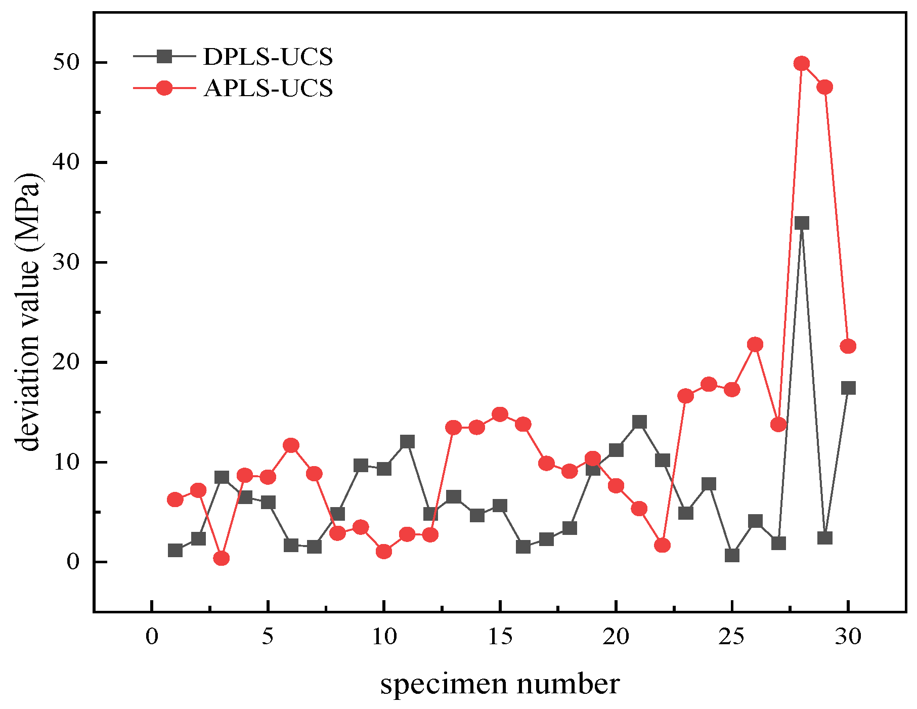
  • Through comparison, it is found that model M2 has better prediction performance than model M3, which indicates from the side that the prediction of UCS by using DPLS is more accurate than using APLS. If DPLS and APLS cannot be obtained simultaneously at the engineering site, the point load test method of diametral loading can be preferred.

Supplementary Materials

The following are available online at https://www.mdpi.com/article/10.3390/min11121387/s1, Table S1: Record of data indexes for uniaxial compression strength test, Table S2: Record of data indexes for diametral point load strength, Table S3: Record of data indexes for axial point load strength.

Author Contributions

S.L. and Y.W. provided experimental ideas and carried out the experiment; X.X. directed and assisted the experiment; S.L. wrote the paper. All authors have read and agreed to the published version of the manuscript.

Funding

This research received no external funding.

Data Availability Statement

The source data can be obtained in the article.

Conflicts of Interest

The authors declare no conflict of interest.

References

  1. Wu, A.Q.; Wang, B. Engineering rock mass classification method based on rock mass quality index BQ for rock slope. Chin. J. Rock Mech. Eng. 2014, 33, 699–706. [Google Scholar] [CrossRef]
  2. Sha, P.; Zhang, Q.T.; Lin, J.; Wu, F.Y. In-situ estimation of uniaxial compression strength of igneous rock based on point load strength. Rock Soil Mech. 2020, 1–10. [Google Scholar] [CrossRef]
  3. Broch, E.; Franklin, J.A. The point-load strength test. Int. J. Rock Mech. Min. Sci. Geomech. Abstr. 1972, 9, 669–697. [Google Scholar] [CrossRef]
  4. Kohno, M.; Maeda, H. Relationship between point load strength index and uniaxial compressive strength of hydrothermally altered soft rocks. Int. J. Rock Mech. Min. Sci. 2012, 50, 147–157. [Google Scholar] [CrossRef]
  5. Kong, F.; Shang, J. A Validation Study for the Estimation of Uniaxial Compressive Strength Based on Index Tests. Rock Mech. Rock Eng. 2018, 51, 2289–2297. [Google Scholar] [CrossRef]
  6. Bieniawski, Z.T. Estimating the strength of rock materials. J. South. Afr. Inst. Min. Metall. 1974, 74, 312–320. [Google Scholar] [CrossRef]
  7. ISRM. Suggested method for determining point load strength. Int. J. Rock Mech. Min. Sci. Geomech. Abstr. 1985, 22, 51–60. [Google Scholar] [CrossRef]
  8. ASTM. Standard Test Method for Determination of the Point Load Strength Index of Rock and Application to Rock Strength Classification. Test Designation D5731−95 Annual Book of ASTM Standards; American Society for Testing and Materials: West Conshohocken, PA, USA, 1995; p. 2. [Google Scholar]
  9. Tsiambaos, G.; Sabatakakis, N. Considerations on strength of intact sedimentary rocks. Eng. Geol. 2004, 72, 261–273. [Google Scholar] [CrossRef]
  10. Basu, A.; Kamran, M. Point load test on schistose rocks and its applicability in predicting uniaxial compressive strength. Int. J. Rock Mech. Min. Sci. 2010, 47, 823–828. [Google Scholar] [CrossRef]
  11. Wong, R.H.; Chau, K.; Yin, J.-H.; Lai, D.T.; Zhao, G.-S. Uniaxial compressive strength and point load index of volcanic irregular lumps. Int. J. Rock Mech. Min. Sci. 2017, 93, 307–315. [Google Scholar] [CrossRef]
  12. Vallejo, L.E.; Welsh, R.A.; Robinson, M.K. Correlation between unconfined compression and point load strengths for Appalachian rocks. In The 30th US Symposium on Rock Mechanics (USRMS); Rock Mechanics Association: Alexandria, VA, USA, 1989; pp. 461–468. [Google Scholar]
  13. Quane, S.L.; Russell, K. Rock strength as a metric of welding intensity in pyroclastic deposits. Eur. J. Miner. 2003, 15, 855–864. [Google Scholar] [CrossRef]
  14. Kılıç, A.; Teymen, A. Determination of mechanical properties of rocks using simple methods. Bull. Int. Assoc. Eng. Geol. 2008, 67, 237–244. [Google Scholar] [CrossRef]
  15. Sabatakakis, N.; Koukis, G.; Tsiambaos, G.; Papanakli, S. Index properties and strength variation controlled by microstructure for sedimentary rocks. Eng. Geol. 2008, 97, 80–90. [Google Scholar] [CrossRef]
  16. Yilmaz, I.; Yuksek, G. Prediction of the strength and elasticity modulus of gypsum using multiple regression, ANN, and ANFIS models. Int. J. Rock Mech. Min. Sci. 2009, 46, 803–810. [Google Scholar] [CrossRef]
  17. Diamantis, K.; Gartzos, E.; Migiros, G. Study on uniaxial compressive strength, point load strength index, dynamic and physical properties of serpentinites from Central Greece: Test results and empirical relations. Eng. Geol. 2009, 108, 199–207. [Google Scholar] [CrossRef]
  18. Li, D.; Wong, L.N.Y. Point Load Test on Meta-Sedimentary Rocks and Correlation to UCS and BTS. Rock Mech. Rock Eng. 2012, 46, 889–896. [Google Scholar] [CrossRef]
  19. Mishra, D.; Basu, A. Estimation of uniaxial compressive strength of rock materials by index tests using regression analysis and fuzzy inference system. Eng. Geol. 2013, 160, 54–68. [Google Scholar] [CrossRef]
  20. Fu, Z.L.; Wang, L. Comparative experimental research on point load strength, uniaxial compression strength and tensile strength for rocks in roof and floor of coal seam. Chin. J. Rock Mechan. Eng. 2013, 32, 88–96. [Google Scholar]
  21. Kahraman, S. The determination of uniaxial compressive strength from point load strength for pyroclastic rocks. Eng. Geol. 2014, 170, 33–42. [Google Scholar] [CrossRef]
  22. Anping, L.; Yangshu, L.; Ming, Z. Study on relationship between poit load strength and uniaxial compressive strength of rock. Non-Ferrous Metals 2014, 66, 53–58. [Google Scholar]
  23. Zhang, J.M.; Tang, Z.C.; Liu, Q.S. Relation between point load index and uniaxial compression strength for igneous rock. Rock Soil Mech. 2015, 36, 595–602. [Google Scholar] [CrossRef]
  24. Yin, J.-H.; Wong, R.H.; Chau, K.; Lai, D.T.; Zhao, G.-S. Point load strength index of granitic irregular lumps: Size correction and correlation with uniaxial compressive strength. Tunn. Undergr. Space Technol. 2017, 70, 388–399. [Google Scholar] [CrossRef]
  25. Lin, J.; Sha, P.; Wu, F. Correlation Between Point Loading Index and Uniaxial Compression Strength of Rock-like Material Based on Size Effect. J. Yangtze River Sci. Res. Inst. 2018, 35, 34–44. [Google Scholar]
  26. Chen, J.Q.; Wei, Z.A. Comparison of rock strength from different point load tests and the uniaxial compression strength. Chin. J. Geol. Hazard Control 2018, 29, 72–77. [Google Scholar] [CrossRef]
  27. Li, H.P.; Wu, Y.Y.; Ge, C. The relation between point load strength and compression and tensile strength of marble. Sci. Technol. Eng. 2019, 19, 294–299. [Google Scholar]
  28. Zhang, C.L.; Zhang, C.P.; Xu, J. Comparison Test of Rock Point Load Strength and Uniaxial Compres-sion Strength. Chin. J. Undergr. Space Eng. 2015, 11, 447–451. [Google Scholar]
  29. Fan, J.; Guo, Z.; Tao, Z.; Wang, F. Method of equivalent core diameter of actual fracture section for the determination of point load strength index of rocks. Bull. Int. Assoc. Eng. Geol. 2021, 80, 4575–4585. [Google Scholar] [CrossRef]
  30. Mozumder, R.A.; Laskar, A.I. Prediction of unconfined compressive strength of geopolymer stabilized clayey soil using Artificial Neural Network. Comput. Geotech. 2015, 69, 291–300. [Google Scholar] [CrossRef]
  31. Heidari, M.; Khanlari, G.R.; Kaveh, M.T.; Kargarian, S. Predicting the Uniaxial Compressive and Tensile Strengths of Gypsum Rock by Point Load Testing. Rock Mech. Rock Eng. 2012, 45, 265–273. [Google Scholar] [CrossRef]
  32. Shao, Y.; Yan, C.H.; Ma, Q.H. Correlation Analysis of Dayangshan Rock Strength in Suzhou. J. Yangtze River Sci. Res. Inst. 2015, 32, 107–110. [Google Scholar]
  33. Zhang, Y.Y.; Li, K.G. The Correlation Between the Point Load Strength and Uniaxial Compression Strength of Several Kinds of Rocks. Metal Mine 2017, 19–23. [Google Scholar]
  34. Zhang, Y.; Zhao, G.F.; Wei, X.; Li, H. A multifrequency ultrasonic approach to extracting static modulus and damage characteristics of rock. Int. J. Rock Mech. Min. Sci. 2021, 148, 104925. [Google Scholar] [CrossRef]
  35. Lei, S.; Kang, H.P.; Gao, F.Q.; Zhang, X. Point load strength test of fragile coal samples and predictive analysis of uniaxial compression strength. Coal Sci. Technol. 2019, 47, 107–113. [Google Scholar] [CrossRef]
  36. Liu, Q.S.; Zhao, Y.F.; Zhang, X.P.; Kong, X.X. Study and discussion on point load test for evaluating rock strength of TBM tunnel constructed in Limestone. Rock Soil Mech. 2018, 39, 977–984. [Google Scholar] [CrossRef]
  37. Ministry of Housing and Urban Rural Development of the People’s Republic of China. GB/T 50218-2014 Standard for Engineering Classification of Rock Mass; China Planning Press: Beijing, China, 2014.
  38. Ministry of Housing and Urban Rural Development of the People’s Republic of China. GB/T 50266-2013 Standard for Test Methods of Engineering Rock Mass; China Planning Press: Beijing, China, 2013.
  39. Gupta, D.; Natarajan, N. Prediction of uniaxial compressive strength of rock samples using density weighted least squares twin support vector regression. Neural Comput. Appl. 2021, 33, 15843–15850. [Google Scholar] [CrossRef]
  40. Sain, S.R.; Vapnik, V.N. The Nature of Statistical Learning Theory. Technometrics 1996, 38, 409. [Google Scholar] [CrossRef]
  41. Kang, F.; Xu, Q.; Li, J. Slope reliability analysis using surrogate models via new support vector machines with swarm intelligence. Appl. Math. Model. 2016, 40, 6105–6120. [Google Scholar] [CrossRef]
  42. Zhou, J.; Huang, S.; Wang, M.; Qiu, Y. Performance evaluation of hybrid GA–SVM and GWO–SVM models to predict earthquake-induced liquefaction potential of soil: A multi-dataset investigation. Eng. Comput. 2021, 1–19. [Google Scholar] [CrossRef]
  43. Li, E.; Zhou, J.; Shi, X.; Armaghani, D.J.; Yu, Z.; Chen, X.; Huang, P. Developing a hybrid model of salp swarm algorithm-based support vector machine to predict the strength of fiber-reinforced cemented paste backfill. Eng. Comput. 2020, 37, 3519–3540. [Google Scholar] [CrossRef]
  44. Syah, R.; Ahmadian, N.; Elveny, M.; Alizadeh, S.M.; Hosseini, M.; Khan, A. Implementation of artificial intelligence and support vector machine learning to estimate the drilling fluid density in high-pressure high-temperature wells. Energy Rep. 2021, 7, 4106–4113. [Google Scholar] [CrossRef]
  45. Joana, C.; Petra, T.; Maisa, N.; Timo, J.; Vahid, F. Machine-learning models for activity class prediction: A comparative study of feature selection and classification algorithms. Gait Posture 2021, 89, 45–53. [Google Scholar]
  46. Wang, Y.; Qiao, C.S.; Sun, C.H.; Liu, K.Y. Forecasting model of safe thickness for roof of karst cave tunnel based on support vector machines. Rock Soil Mech. 2006, 1000–1004. [Google Scholar] [CrossRef]
  47. Huang, W.Y.; Tong, M.M.; Ren, Z.H. Nonlinear combination forecast of gas emission amount based on SVM. J. China Univ. Min. Technol. 2009, 38, 234–239. [Google Scholar]
  48. Hsu, C.W.; Lin, C.J. A comparison of methods for multiclass support vector machines. IEEE Trans. Neural Netw. 2002, 13, 415–425. [Google Scholar]
  49. Wang, Q.; Sun, H.B.; Jiang, B. A method for predicting uniaxial compressive strength of rock mass based on digital drilling test technology and support vector machine. Rock Soil Mech. 2019, 40, 1221–1228. [Google Scholar] [CrossRef]
  50. Teymen, A.; Mengüç, E.C. Comparative evaluation of different statistical tools for the prediction of uniaxial compressive strength of rocks. Int. J. Min. Sci. Technol. 2020, 30, 785–797. [Google Scholar] [CrossRef]
Figure 1. The main test process, in which (a) is the diametral point load test specimen, (b) is the uniaxial compression test specimen, and (c) is the axial point load test specimen. (The test equipment mainly adopts HCT-206A rock true triaxial compression tester produced by Shenzhen Wance Test Equipment Co., Ltd., Shenzhen, China and STDZ-3 digital display point load tester produced by Zhejiang Geotechnical Instrument Manufacturing Co., Ltd., Zhejiang, China).
Minerals 11 01387 g001
Figure 2. Q-Q diagram for normality test of test data, (a) UCS, (b) DPLS, (c) APLS.
Minerals 11 01387 g002
Figure 3. Fitting curve between UCS and PLS for (a) is DPLS, (b) is APLS.
Minerals 11 01387 g003
Figure 4. The error comparison chart between the UCS predicted value and experimental value generated by the exponential function formula.
Minerals 11 01387 g004
Figure 5. Schematic diagram of SVM model for predicting UCS using DPLS and APLS.
Minerals 11 01387 g005
Figure 6. Comparison between the real and predicted values of model M1, (a) M1 training set and (b) M1 prediction set.
Minerals 11 01387 g006
Figure 7. Comparison of the real value and predicted value of model M2 and model M3, (a) M2 training set, (b) M2 prediction set, (c) M3 training set and (d) M3 prediction set.
Minerals 11 01387 g007aMinerals 11 01387 g007b
Table 1. Statistical table of correlation between PLS and UCS (arranged by year).
NO.YearAuthorsRock TypeEquationsR2
11985ISRM [7]granite, marble et al.R = (20~25) Is(50)-
21989Vallejo et al. [12]graniteR = 12.6 Is(50)R = 17.4 Is(50)-
32003Quane, S.L., Russell, J.K. [13]welded ignimbriteR = 3.86 (Is(50))2 + 5.65 Is(50)-
42004Tsiambaos et al. [9]limestoneR = 7.3 (Is(50))1.710.90
52008KiliÇ, A., Teymen, A. [14]limestone, tuff et al.R = 100 ln(Is(50)) + 13.90.99
62008Sabatakakis, N. et al. [15]limestone, sandstoneR = 28 Is(50)0.73
72009Yilmaz, Yuksek [16]sandstone, conglomerateR = 12.4 Is(50) − 9.080.85
82009Diamantis, K, et al. [17]serpentinitesR = 16.45 e0.39Is(50)0.89
92010Basu, A. et al. [10]apatiteR = 11.103 Is(50) + 37.660.86
102012Kohno, M., Maeda, H. [4]volcaniclastic, tuffR = 16.4 Is(50)0.90
112013LI.D, Wong, L. [18]metasandstoneR = 21.27 Is(50)-
122013Mishra, D.A., Basu, A. [19]granite, schist, sandstoneR = 14.63 Is(50)0.94
132013FUZhiliang, et al. [20]sandstone, mudstoneR = 7.201 Is(50) + 14.074 (Axial)
R = 13.938 Is(50) + 17.529 (Diametral)
0.99
0.97
142014Kahraman, S. [21]ignimbriteR = 7.73 (Is(50))1.250.91
152014LI anping et al. [22]sandstone, mudstoneR = 14.933 ln(Is(50)) + 89.0120.79
162015ZHANG Jianming et al. [23]granite, andesiteR = −0.66 (Is(50))2 + 21.15 Is(50)0.94
172017Jian-Hua Yin et al. [24]graniteR = 21.605 Is(50)0.74
182017Robina H.C. Wong et al. [11]granite, tuffR = 18.897 Is(50)0.87
192018LIN jun et al. [25]cement blockR = 29.87 Is(50) − 2.2420.99
202018CHEN Jiaqi, WEI Zuoan [26]limestone, sandstoneR = 22.72 (Is(50))0.82 (Irregular)
R = 26.24 (Is(50))0.72 (Regular)
0.86
212019LI Hongpeng et al. [27]marbleR = 21.28 Is(50)-
222020SHA Peng et al. [2]igneousR = 0.14 (Is(50))2 + 13.25 Is(50)0.93
Table 2. Two main parameters used in the SVM model.
Model NamePenalty Factor CSensitive Parameter γ
M1256.751.13
M2226.271.41
M3362.042.38
Publisher’s Note: MDPI stays neutral with regard to jurisdictional claims in published maps and institutional affiliations.

