Abstract
Hyperspectral technology has been used to identify pigments that adhere to the surfaces of polychrome artifacts. However, the colors are often produced by the mixing of pigments, which requires that the spectral characteristics of the pigment mixtures be considered before pigment unmixing is conducted. Therefore, we proposed an experimental approach to investigate the nonlinear degree of spectral reflectance, using several mixing models, and to evaluate their performances in the study of typical mineral pigments. First, five mineral pigments of azurite, malachite, cinnabar, orpiment, and calcite were selected to form five groups of samples, according to their different mass ratios. Second, a fully constrained least squares algorithm based on the linear model and three algorithms based on the nonlinear model were employed to calculate the proportion of each pigment in the mixtures. We evaluated the abundance accuracy as well as the similarity between the measured and reconstructed spectra produced by those mixing models. Third, we conducted pigment unmixing on a Chinese painting to verify the applicability of the nonlinear model. Fourth, continuum removal was also introduced to test the nonlinearity of mineral pigment mixing. Finally, the results indicated that the spectral mixing of different mineral pigments was more in line with the nonlinear mixing model. The spectral nonlinearity of mixed pigments was higher near to the wavelength corresponding to their colors. Meanwhile, the nonlinearity increased with the wavelength increases in the shortwave infrared bands.
1. Introduction
The use of pigment analysis to determine the type and proportion of pigments on the surface of artifacts has become a research focus. In ancient times, pigments were usually made of chromatic materials existing in nature. Mineral pigments were commonly used in polychrome cultural relics with relatively stable properties [1]. Some mineral pigments, such as malachite and azurite, exhibit unique absorption specificities that can be used to identify them [2]. The different colors on the surface of polychrome artifacts are created by pigments being mixed together or layered on top of one another. The shape and absorption position of the spectrum are related to the spectra and proportions of its components. It is hard to recognize the types of pigment using only the human eye. Thus, the identification of the pigments used on the surfaces of artifacts needs modern techniques.
In recent decades, many non-invasive techniques have been employed on polychrome artifacts to provide information about the types and the distributions of pigments on the entire surfaces of artifacts [3,4,5]. Many of these techniques, such as X-ray fluorescence (XRF) and Raman spectroscopy, focus on elemental and molecular analysis for the recognition of the pigments in the mixture. For instance, Delaney et al. [6] combined reflectance, molecular fluorescence imaging spectroscopy, and macroscale X-ray fluorescence scanning on Johannes Vermeer’s Girl with a Pearl Earring (c. 1665, Mauritshuis) to obtain a comprehensive understanding of the distribution of pigments and how the coloration of the painting was achieved. Additionally, pigment analysis with spectrophotometry and Fiber optics reflectance spectroscopy (FORS) can provide the optical material characteristics for the study of spectral reflectance [7,8]. They have been increasingly employed for the identification of pigments in mixtures, due to their portability and ability to perform noninvasive investigation. For instance, Fonseca et al. [9] employed reflectance spectroscopy to noninvasively identify madder and cochineal pigments on oil works. The features in the first derivative transformation of the FORS spectra were used for pigment identification. Among them, hyperspectral technology has been applied to the pigment identification field, with the advantages of its noninvasive qualities, no need for sampling, high spectral resolution, and full surface coverage [10]. They can be divided into two categories: single pigment identification and pigment unmixing. The first directly compares the measured spectrum with spectral databases to obtain the type of possible pigment; the second can provide more than one possible pure pigment, as well as the proportion of each pigment in the mixture.
Single pigment identification calculates the similarity between an unknown spectrum and standard spectra in a spectral library based on different spectral matching methods, such as spectral angle mapping (SAM), spectral feature fitting (SFF), or binary encoding (BE). The pigment with the most similar spectrum will be considered the pigment type at that point. Many studies have applied this type of method to identify the pigments on the surfaces of artifacts. Wang et al. [11] acquired hyperspectral images that covered 400–1000 nm and their spectral information from the wall paintings at Jokhang Monastery in Lhasa, Tibet, China. The methods of SFF, SAM and BE were used together to identify the pigments of azurite, malachite, red lead and cinnabar by comparing their reflectance spectral curves, characteristic reflectance peaks, first derivative peaks, and spectral similarity with standard pigments. Wu et al. [12] used a shortwave infrared imaging spectrometer that covered 1000–2500 nm to analyze cultural relics. An ancient painting that was created to celebrate the 80th birthday of the Empress Dowager Chongqing in the Qianlong period served as a sample. They highlighted the absorption features on the spectral curve by continuum removal and then used SAM to identify azurite pigment in the clothes of the characters. Li et al. [13] proposed an automatic identification method for the extraction of painting boundaries and the identification of pigment composition based on the visible spectral images of colored relics. They applied superpixel segmentation to extract the painting boundary and compare the proximity between the geometric profiles of the unknown spectrum from each superpixel and the known spectrum from a deliberately prepared database. This method assumes that the color on one point, observed by the naked eyes or by instruments, is formed by a single pigment. This assumption is difficult to satisfy, often the patterns on the surface of artifacts are a combination of more than one pigment in different proportions.
Based on the assumption that pigments are often mixed in painting, the second category is pigment unmixing, which can provide several possible types of pigment and their proportions for each pixel in the hyperspectral data at the same time. A single pixel in the hyperspectral image may be described as a mixture of the reflectance spectra of the pure pigments present in this pixel. The pure pigment spectra are regarded as endmember spectra and the proportion of the pure pigment is regarded as its abundance. The process of obtaining the type and proportions of pigment endmembers in a mixed spectrum is similar to the unmixing of mixed pixels in the hyperspectral image. Early works mainly focused on the linear mixing model (LMM), due to its simplicity and definite physical meaning [14]. This can be subdivided into three ways of performing linear unmixing for a pigment mixture. The first extracts the endmember spectra and obtains their corresponding abundances step by step. Endmember extraction and abundance inversion are relatively independent algorithms, which can be developed separately. For instance, Deborah et al. [15] employed fully constrained least squares (FCLS) for the pigment mapping of The Scream (1893) painting, under the assumption that the endmembers were known. This approach can recognize the mixture of some percentage of different pigments. Bai et al. [16] used the Gram Matrix and Max-D techniques to estimate the dimensionality in HSI data as well as extract the endmember spectra. After extracting endmembers, the nonnegative linear least squares algorithm and the K-means algorithm were used to estimate the pigment classification maps. They provided a novel pigment mapping approach to study the material diversity of cultural heritage artifacts by using a hyperspectral image. Zhao et al. [17] performed the ratio spectra derivative spectrophotometry algorithm using some bands with a high degree of linear mixing to estimate the abundance of components in a mixture. The accuracy of the abundance inversion was much higher than that obtained using the FCLS method. The second kind of method can extract endmembers and calculate abundance simultaneously, such as independent component analysis (ICA). Under the assumption that the mixed spectrum is a linear combination of multisource signals, these algorithms were applied to the quantitative analysis of pigment mixture [18]. For instance, Wang et al. [19] first used ICA to obtain the pure pigment spectra from mixtures, and then estimated the Kubelka-Munk (K-M) theory to obtain the proportions of pure pigments. This method is suitable for the analysis of mixed pigments and has the potential for application to color material restoration in the cultural heritage conservation field. The third kind applies sparse modeling by building a pigment spectral library. They use a complete dictionary to decompose the measured spectrum of a pigment into a sparse coefficient vector that directly corresponds to the abundances of pure pigment in the mixture. For instance, Rohani et al. [20] utilized sparse unmixing via variable splitting and augmented Lagrangian to detect hematite and indigo pigments on the surface of a Roman–Egyptian portrait. However, the linearity assumption in the pigment spectral mixing is not satisfied. The accuracy of pigment unmixing based on the LMM will be limited if LMM cannot describe the pigment spectral mixing well.
In recent years, some nonlinear mixing models (NLMM) have also been introduced into pigment identification. The K-M model [21] can predict the reflectance spectra for pigment mixtures in semitransparent or opaque paint layers from a weighted sum of the ratios between the absorption and scattering coefficients of each pigment. Taufique et al. [22] utilized the single-constant K-M theory for the classification of green pigments in the Selden Map, China, created in the early 17th century. They first transformed the spectra extracted into the ratio of absorption and scattering and then performed linear unmixing using the non-negative least square technique to obtain the abundance of pigments. This method provided a tool to estimate pigment diversity and spatial distribution within historical artifacts where prior information is unknown. Rohani et al. [23] associated the two-constant K-M model with a deep neural network classifier to realize pigment recognition and quantitative estimation of concentration on hyperspectral data. In addition, with the development of deep learning, some scholars have used neural network models to unmix pigments. For instance, Bai [24] proposed a new neural network and applied it to two historical maps, the Gough Map of Britain and the Selden Map of China. The method makes full use of the spatial and spectral characteristics to achieve pigment mapping. Kleynhans et al. [25] created a one-dimensional convolutional neural network that was trained by the surface pigment dataset of four ancient paintings. This was then used to test a 14th century painted manuscript.
The studies mentioned above applied different linear or nonlinear models to improve the performances of abundance inversion on pigment mixtures. The accuracy abundance of pigment mixtures is hindered by the complexities of the spectral mixing characteristics. However, it is more important to quantitatively investigate the nonlinear degree of spectra mixed by different pigments before conducting pigment unmixing. Therefore, we developed an experimental approach to investigate the spectral mixing characteristics of typical pigments to help select the most suitable method and achieve higher accuracy in pigment identification.
In this study, each group of samples was made by mixing two pigments in different mass ratios, which were selected from the mineral pigments that were commonly used in Chinese painting. The samples were a mixture of azurite and malachite, azurite and orpiment, cinnabar and orpiment, cinnabar and calcite, and orpiment and calcite. Four mixing models were selected to evaluate the nonlinear mixing characteristics through an approach composed of three steps. The first step was to evaluate the accuracy of the abundances generated by different algorithms based on the ground truth of concentrations and endmembers in the pigment samples. In the second step, the reconstructed spectra were obtained by the abundances inversed by different models. The similarity between the measured and reconstructed spectra were compared to evaluate the nonlinear mixing degree in the whole and each spectral band. In the third step, the best model was applied to a Chinese painting, aiming to evaluate the ability of this model to estimate the pigment concentrations.
This paper is organized as follows: In Section 1, we start with an overall introduction of the study and a brief review of related works. Section 2 provides a detailed description of sample preparation, including the pigment selection, mockup making and data acquisition process. Section 3 introduces the overall scheme as well as the investigated models including linear and nonlinear models, while Section 4 shows the experiments results. In Section 5, other methods are performed in the study of mineral pigments and the obtained results are discussed. In Section 6, the conclusion is briefly summarized and future work is outlined.
2. Materials
2.1. Sample Preparation
2.1.1. Pigment Selection
Through repeated practice over a long time, the usage of pigments has gradually developed certain rules and painting skills. After careful investigation and comparison, we selected azurite, malachite, cinnabar, orpiment, and calcite as the study objects, which are the mineral pigments most commonly used in traditional Chinese paintings. They are the representative pigments in cyan, green, red, yellow and white colors, respectively. For example, in Chinese landscape painting, azurite is often used to spot dark areas of mountains and rocks to enhance the contrast between brightness and darkness. Malachite is often used to draw green leaves and bright areas of mountains and rocks. Cinnabar is often used to draw red autumn leaves, flowers, pavilions, etc. Orpiment is often used to draw autumn scenes with leaves and moss, while calcite is often used as a white pigment, which can be mixed with other pigments to dilute the color to obtain a multilayer effect.
To ensure the pigments’ quality, pigments in powder form produced by Jiang Sixutang, a famous traditional pigment brand established 300 years ago, were selected to produce mixed pigment samples to study the mixing characteristics of different mineral pigments.
2.1.2. Binder Selection
Since mineral pigment powder cannot be directly drawn on the surface of the substrate, some binder materials are used to enhance adhesion in traditional painting, including animal protein, polysaccharides or lipids [26]. In this experiment, the gelatin produced by Jiang Sixutang was used as the binder, which is a kind of binding material that is similar to the traditional animal protein, used in ancient times [27].
2.1.3. Making the Mockups
Raw rice paper, without aluminum on the surface, produced by a famous brand called Rongbaozhai, was selected as the substrate. In this study, we designed five single pigment samples: azurite, malachite, cinnabar, orpiment and calcite. The five series of pigment mixtures were a mixture of azurite and malachite, a mixture of azurite and orpiment, a mixture of cinnabar and orpiment, a mixture of cinnabar and calcite and a mixture of orpiment and calcite. Each sample block was designed to be 4 × 4 cm, which provides a large enough area to acquire spectral data. The mixtures can be made through the following steps. First, the powder pigments were weighed by using an electronic balance with 0.001 g precision in the different mass ratios. Each group mixture included seven mixed-pigment samples, in which the total mass of a mixture, by weight in the laboratory, was 1 g. Second, the same amount of gelatin was added, about 2 mL. Third, they were stirred and mixed so that the gelatin and pigments were fully integrated. Fourth, the mixtures were painted once on the raw rice paper with a brush. In this way, we obtained five pure pigment samples, as shown in Figure 1, as well as five groups of mixture samples, as shown in Figure 2.
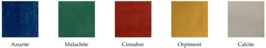
Figure 1.
The sample blocks of pure pigments.
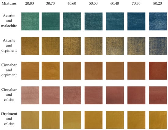
Figure 2.
The five groups of sample blocks with mixed pigments.
A Chinese painting was utilized to further study the combination of pigment mixtures in different types and proportions. It was drawn with several commonly used pigments, based on traditional Chinese painting skills, as shown in Figure 3. We selected the raw rice paper as the substrate and the gelatin as the binding material. The pigments used during painting were recorded as reference data. In this painting, first, the shape of the leaves were outlined with black ink. Second, the green leaves were filled with the pigment malachite, and the blue leaves were filled with the pigment azurite. Third, the veins were delineated with ink again. Finally, each leaf was rendered with light ink. The red petals were drawn by mixing cinnabar and clam meal. They were painted using the side edge of the brush, with clam meal in its middle position and cinnabar in its tip position, causing a variation in color from dense to light. The center of the red flower was drawn with the red pigment eosin. The stamens were drawn with the yellow pigment orpiment. The branches were drawn by mixing malachite and ocher.
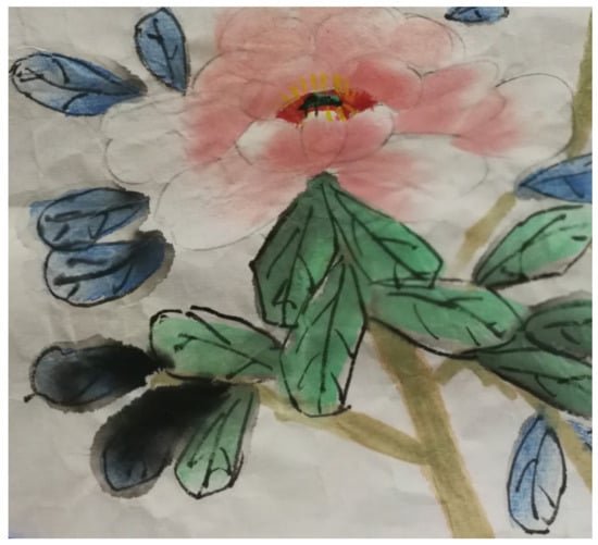
Figure 3.
A Chinese painting in true color, which was drawn with several pigments.
2.2. Data Acquisition and Preprocessing
In this study, the instrument used to acquire the spectral data was an Analytical Spectral Devices (ASD) FieldSpec 4 portable spectroradiometer (Analytical Spectral Devices Inc., Boulder, CO, USA). The main specifications of this instrument are shown in Table 1. The reflectance spectra of the samples were measured using a well-sealed probe with an internal halogen light source for illumination under a dark room. The spectral reflectance was normalized with a white standard reflectance measured on a Spectralon plate (Labsphere, Inc., North Sutton, NH, USA). Each sample was measured 15 times to prevent ambient light and reduce operational error. The measured reflectance spectra were averaged with ViewSpecPro software (ViewSpecPro 6.2).

Table 1.
Specifications of ASD FieldSpec 4 portable spectroradiometer.
The instrument used to capture the hyperspectral image of the Chinese painting was a Themis Vision Systems VNIR400H (Themis Vision Systems Inc., Long Beach, MS, USA), a pushbroom scanning hyperspectral imaging system. The main specifications of this instrument are shown in Table 2. This system uses two halogen lamps close to the solar spectrum for illumination. During data acquisition, the lights were fixed on the left and right sides of the camera. The camera and lights were placed vertically with respect to the painting. The collected hyperspectral image was resized to 1004 × 953 pixels to include the whole picture.
Table 2.
Specifications of hyperspectral imaging spectroradiometer parameters.
The original hyperspectral data are always influenced by the change in environmental parameters and dark current noises. Therefore, it is necessary to reduce the noise using Equation (1)
where is the calibrated data, is the collected original hyperspectral data, is the standard white board data, and is the dark current noise data. Due to the noise being presented more seriously at both ends of the wavelength, the first 50 and last 50 spectral bands were omitted from the data. Thus, we obtained a hyperspectral image with 51–990 bands (405.79–1000.79 nm). The minimum noise fraction (MNF) was performed using ENVI software (ENVI 5.3, Research System Inc., Boulder, CO, USA). The former 10 components with more than 95% cumulative information content were selected to perform inverse MNF transformation to restore hyperspectral data dimension and achieve data denoising.
3. Methods
The overall process of studying the nonlinear mixing characteristics of the reflectance spectra of typical mineral pigments is given in Figure 4.
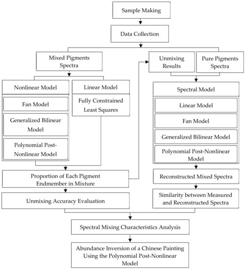
Figure 4.
The overall process of the study.
The experiment can be carried out as follows:
- (1)
- Pigment sample preparation and data acquisition. Samples of mixed pigment in different mass ratios and a Chinese painting were produced as study objects. Moreover, the progress of data acquisition of those objects is given in detail in Section 2.2.
- (2)
- Accuracy analysis of abundances estimated by linear and nonlinear algorithms. For each mixture sample, the measured spectrum was decomposed to obtain the abundance of each pigment endmember, under the assumption that the pigment endmembers are known. The FCLS based on the linear mixing model and the Fan model (FM), the generalized bilinear model (GBM) and polynomial post-nonlinear model (PPNM) algorithms based on the nonlinear mixing model, were selected and adapted to estimate the abundance of each pigment in the mixed samples. Then, the abundance accuracies of linear and nonlinear algorithms were compared to explore the spectral nonlinearity of the mixed pigment.
- (3)
- The similarity analysis between measured and reconstructed mixed spectra. Based on the measured spectra of pure pigments and their corresponding abundance in a mixture calculated by different algorithms, the reconstructed spectra can be obtained by the LMM, the FM, GBM and PPNM, respectively. Moreover, by comparing the similarities between the reconstructed spectra and the measured spectra of the corresponding mixed pigments, the spectral characteristics of pigment mixing were analyzed.
- (4)
- Spectral mixing characteristics analysis. According to the above spectral unmixing analysis and reconstructed mixed spectra analysis, the spectral nonlinearity of the mixed pigments was discussed for the five typical mineral pigments.
- (5)
- Experiment with a Chinese painting. The PPNM algorithm was selected to study a Chinese painting to evaluate the nonlinear model’s ability to correctly estimate the pigments and their relative concentrations.
3.1. Spectral Characteristics
The spectra of pure pigment and mixed pigment samples are shown in Figure 5.
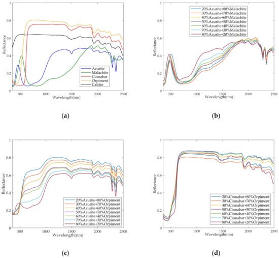
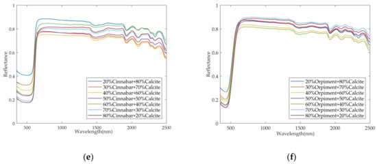
Figure 5.
Spectra of pure pigments and mixed pigments in different mass ratios: (a) pure pigment spectra; (b) azurite and malachite mixed spectra; (c) azurite and orpiment mixed spectra; (d) cinnabar and orpiment mixed spectra; (e) cinnabar and calcite mixed spectra; (f) orpiment and calcite mixed spectra.
Figure 5a illustrates the unique spectral characteristics for the five mineral pigments, which cover the visible and shortwave infrared range of the spectrum (350–2500 nm). Azurite is composed of subcarbonate with the formula 2CuCO3·Cu (OH)2, whose spectrum shows a relatively sharp band at about 460 nm and a broad strong absorption band centered at about 800 nm. Different absorption bands at about 1500 nm, 1930 nm, 2050 nm, 2285 nm, and 2355 nm are characteristic of the functional groups CO32− and OH−. Malachite is composed of subcarbonate with the formula CuCO3·Cu (OH)2, whose spectrum shows a relatively sharp band at about 526 nm. The typical strong absorption band is centered at about 800 nm, which is the characteristic of the main cation Cu2+. A series of absorption bands are seen at about 1930 nm, 2050 nm, 2270 nm, and 2350 nm. Cinnabar is composed of mercuric sulfide with the formula HgS, presenting a steep sigmoid-shaped spectrum with an inflection point at about 600 nm. Orpiment is composed of arsenic trisulfide with the formula As2S3, presenting a simple sigmoid shape with an inflection point at about 480 nm. Calcite is composed of calcium carbonate with the formula CaCO3, whose spectrum gradually increases from visible near-infrared bands and has absorption features of CO32− at about 1900 nm, 2350 nm, and 2500 nm.
3.2. Absorption/Scattering Characteristics
According to the Kubelka-Munk theory [28], the relationship between the reflectance spectra of a substance and its absorption and scattering coefficients can be expressed as in Equation (2)
where is the pigment spectrum measured, is the absorption coefficient, and is the scattering coefficient. The ratio between absorption and scattering coefficients can be calculated using Equation (3)
In this way, the values of the five mineral pigments were computed. Figure 6 shows the ratio between the absorption and scattering coefficients of the different mineral pigments for five groups of mixed samples.
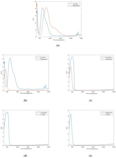
Figure 6.
The ratio between the absorption and scattering coefficients of different mineral pigments: (a) azurite and malachite pigments; (b) azurite and orpiment pigments; (c) cinnabar and orpiment pigments; (d) cinnabar and calcite pigments; (e) orpiment and calcite pigments.
In these five groups of mixed samples, the correlation between the absorption and scattering characteristics of the component pigments is clear. As can be seen from Figure 6a,b, for azurite and malachite pigments as well as azurite and orpiment pigments, there is less overlap between the curves. There is basically no overlap at the peak position between the curves. Their curves are obviously different. In addition, for the other mineral pigments, as shown in Figure 6c–e, there are many overlaps between the curves of the component pigments. One curve almost completely contains the other curve, with fewer intersections. Therefore, these five groups of samples are not only a common mixture in painting, but also representative of the property. We hope to investigate the nonlinear degree of pigment mixing in different component pigments characterized by the different curves.
3.3. Linear Mixing Model
LMM is a simplified spectral mixing model that works under the assumption that each incident photon interacts with only one component on the surface and that the reflectance spectrum does not mix before entering the sensor [29]. In that case, the spectrum of a mixed pixel can be described as a linear combination of the endmembers’ spectra, which can be expressed in Equation (4)
where is the mixed pigment spectrum measured, is the number of spectral bands, and is the matrix whose columns are the endmember , , and is the number of endmembers in this mixture, is the abundance vector, where is the abundance of the endmember in this pigment mixture, and is the error term.
Moreover, the abundance of each endmember in the LMM must satisfy the following sum-to-one and non-negativity constraints, as shown in Equation (5).
FCLS is the most widely used abundance inversion algorithm based on the LMM [30]. Given the known mixed spectra and the endmembers’ spectra , we can determine the abundance matrix using the FCLS. Based on the constraints in Equation (5), we can perform it according to the following optimization problem, which is given by Equation (6).
3.4. Bilinear Spectral Mixing Model
The bilinear spectral mixing models are an improvement on the LMM, which additionally account for the presence of multiple photon interactions between endmembers by introducing the bilinear term [31]. Each term is represented by the cross-product of the two endmembers as well as the nonlinear coefficient. According to the different nonlinear coefficients and constraints, the bilinear spectral mixing models vary.
3.4.1. Fan Model
In 2009, Fan et al. [32] proposed a new nonlinear model for inferring the abundance of endmembers with hyperspectral images, which only considered the presence of the second-order scattering between endmembers and ignored the influence of higher-order multiple scattering. The FM extended the LMM with the cross-product term which describes spectral interactions between every two endmembers. Moreover, the bilinear terms in the FM are scaled with the respective abundances, reasoning that the probability that each incident photon interacts with two endmembers should be proportional to their corresponding abundances in the mixed pixel [33]. In this case, the FM can be given by Equation (7)
where is the mixed pigment spectrum measured, is the number of spectral bands, is the ith endmember spectrum, is the total number of endmembers in a mixture, is the abundance of the ith endmember in this mixture, is the Hadamard or element-wise product of two endmembers vector, and is the error term. The constraints on the abundance are “sum to one” and “non-negativity”.
3.4.2. Generalized Bilinear Model
In 2011, Halimi et al. [34] proposed the GBM, which improved on the FM by introducing additional parameters to each bilinear term. The parameter indicates the interaction degree between the endmember and , and is constrained in [0,1]. The parameter has an upper bound of 1, reflecting the fact that the interaction term is always smaller than the product of the individual abundances. Moreover, it makes sense to assume to ensure that the measured vector is positive. The GBM model can be given by Equation (8)
when , the GBM reduces to the LMM, and when , the GBM reduces to the FM.
3.4.3. Polynomial Post-Nonlinear Model
In 2012, the PPNM was proposed by Altmann et al. [35], assuming that a second-order polynomial can be used to perform a transformation of the spectrum that is linearly mixed by its endmembers to describe nonlinearities. The PPNM uses parameter to scale the size of the quadratic term, and all bilinear terms in a pixel are multiplied by the same parameter. The PPNM can be given by Equation (9)
where is a parameter to adjust the degree of the nonlinear effect. When , the PPNM reduces to the LMM. It should be noted that both the Fan model and the GBM exclude self-interaction terms such as , while they are included in the PPNM because self-interactions can form an important contribution to the measured spectra [36].
4. Experimental Results
4.1. Abundance Accuracy by Different Methods
Pigment unmixing mainly involves endmember extraction and abundance inversion. The former step is used to determine the types of pigment endmember and their spectra from the spectrum of the mixed pigment, which has been discussed in [37]. The latter step is used to calculate the proportion of each pigment in the mixture. In this study, we assume that the types of pigment endmember and their corresponding spectra are known, and then we use different unmixing algorithms to perform abundance inversion.
The root mean square error (RMSE) was used to evaluate the abundance accuracy of different algorithms. It compares the difference abundances calculated by the four algorithms with those measured by a balance in the laboratory. For each group of mixture, the RMSE can be calculated as follows
where is the ith is abundance of one endmember calculated by the unmixing algorithm, is the ith abundance of the same endmember measured by a balance in the laboratory, and is the number of samples in each group of mixtures ( in this study). The smaller the RMSE, the smaller the error in the abundance inversion and the higher the unmixing accuracy.
By using the spectra of the pure pigments, FCLS based on the LMM as well as the FM, the GBM and PPNM based on the NLMM were carried out on the five groups of mixtures to obtain the abundance values. In practice, the parameter in the GBM is limited to [0, 1], and parameter in the PPNM is limited to [−100,100]. We obtained parameter and MATLAB (The Math Works Inc., Natick, MA, USA) based on the optimization problems mentioned in [34,35]. The abundance results of five groups of mixed pigment samples—azurite and malachite, azurite and orpiment, cinnabar and orpiment, cinnabar and calcite, and orpiment and calcite—are listed in Table 3, Table 4, Table 5, Table 6 and Table 7, respectively. Their RMSE values are also calculated and listed in these tables.
Table 3.
Abundance estimated by different approaches for mixed pigment samples of azurite and malachite.
Table 4.
Abundance estimated by different approaches for mixed pigment samples of azurite and orpiment.
Table 5.
Abundance estimated by different approaches for mixed pigment samples of cinnabar and orpiment.
Table 6.
Abundance estimated by different approaches for mixed pigment samples of cinnabar and calcite.
Table 7.
Abundance estimated by different approaches for mixed pigment samples of orpiment and calcite.
From the abundance inversion results in Table 3, Table 4, Table 5, Table 6 and Table 7, we can observe that the four algorithms performed differently on the different mixed pigments.
- (1)
- For the five groups of pigment mixture, the spectral mixing characteristics showed a certain degree of nonlinearity. The result was consistent with the previous research conclusions on powder pigment mixtures [38]. Furthermore, for the abundance RMSE obtained by the FCLS, the abundance accuracy of the mixture of azurite and malachite listed in Table 3 as well as the mixture of azurite and orpiment listed in Table 4 were much better than that of the other groups of mixtures. The spectral mixing characteristics of the two groups of mixtures were likely to be simpler and less nonlinear. For the other mixtures, the abundance accuracy obtained by the four algorithms was relatively low, especially that obtained by the FCLS. The nonlinearity of these mixtures was of high intensity.
- (2)
- For the four unmixing algorithms, the FCLS provided poor results while the NLMM was the best on the study of five groups of mixtures, particularly the PPNM. The abundance RMSE obtained by the PPNM was almost half of that obtained by the FCLS. The reason the PPNM achieved the best results may be that it took the interaction between the same pigment particles into account. Moreover, the FM and GBM might produce some of the same abundances depending on the parameter value. Their accuracy was also significantly improved compared with the FCLS. Although the abundances were improved by the NLMM, the error was still a little large, which indicated that a more effective NLMM should be developed to fit with the pigment mixing.
- (3)
- For the different component pigments used, the linearity of spectral mixing was better with the mineral pigments that are color pigments, whose curves are obviously different. The linear model may be used directly for these kinds of mixtures when the accuracy requirement is not very strict. On the other hand, when the pigment mixture is composed of mineral pigments with similar curves or white pigment is one of the components, the nonlinear mixing characteristic plays a key role in the measured spectra. In this case, it was necessary to select the nonlinear model to estimate the abundances of pigment endmembers in these mixtures.
4.2. Analysis of Reconstructed Mixed Spectra
After calculating the abundances of each pigment in mixtures, we can use the pure pigments spectra (considered as endmembers) and their abundances to construct a mixed spectrum by the models of LMM, FM, GBM and PPNM, respectively, which we call the reconstructed spectrum. For the LMM, the mixed spectrum can be reconstructed directly based on Equation (4). Likewise, for the other three models, we reconstruct the spectrum based on Equations (7)–(9). For the GBM and PPNM, the calculated parameters and would be used. The similarity between the reconstructed and measured spectra of the corresponding mixed pigments is evaluated by considering the reconstruction error (RE) and the spectral angle distance (SAD). For each group of mixtures, the RE and SAD can be given by Equations (11) and (12)
where is the measured mixed spectrum, is the reconstructed spectrum, and is the number of spectral bands, is the usual Euclidean norm (), and is the inverse cosine operator. The smaller the RE and the SAD, the higher the similarity between the two spectra, and the higher the unmixing accuracy.
The reconstructed spectra were obtained by the linear and nonlinear mixing models. The performance of different models was evaluated by the mean RE and the mean SAD, which were averaged over all samples for each group of mixtures. The results for the five groups of mixed pigment samples—azurite and malachite, azurite and orpiment, cinnabar and orpiment, cinnabar and calcite, and orpiment and calcite—are listed in Table 8.
Table 8.
The mean RE and mean SAD for mixed pigment samples of linear and nonlinear mixing models.
In Table 8, the results indicated that the similarity between the reconstructed and measured spectra obtained by the linear model was poorer than that obtained by the nonlinear models in terms of the mean RE and the mean SAD. Among the four models, the PPNM provided almost the best results, except for the mean SAD of azurite and malachite as well as cinnabar and calcite. The accuracy of the FM and GBM was similar, between the LMM and PPNM. Overall, the nonlinearities occurring in the mixed spectra of different mineral pigments can be better described by the various nonlinear models, especially the PPNM.
To investigate the difference in nonlinearity in the spectral bands, we used the mean reconstruction difference (RD) in the () band . It is given by Equation (13)
where is the reflectance data of the measured spectrum in the band, is the reflectance data of the reconstructed spectrum in the band, and is the number of spectral bands, n is the number of samples in each group of mixtures (n = 7 in this study).
Based on the spectral dimension, value was calculated and compared between the above four models for each group of mixtures. The results are given in Figure 7.
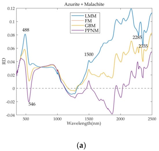
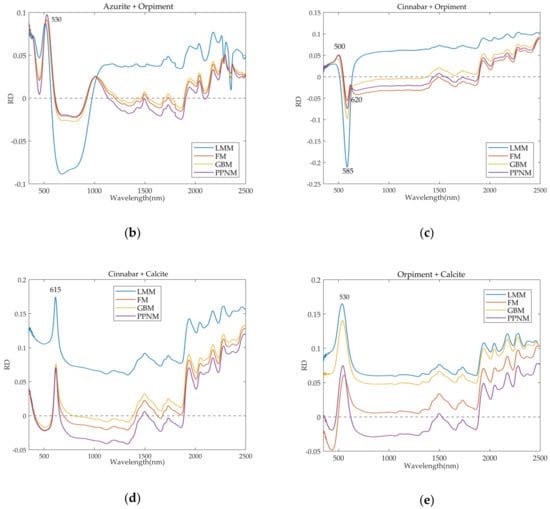
Figure 7.
The mean reconstruction difference at different spectral bands for the five groups of mixed pigments: (a) azurite and malachite; (b) azurite and orpiment; (c) cinnabar and orpiment; (d) cinnabar and calcite; (e) orpiment and calcite.
It can be seen from Figure 7 that the RD of the different pigment mixtures in different spectral bands is different, which reflects the different nonlinear degrees in the bands.
- (1)
- In Figure 7, the wavelengths of the peaks corresponding to the larger RD by the LMM in the five groups of mixed pigments are marked. The peaks indicated that the nonlinear effects were of high intensity around these bands. We also found that in the visible bands, the RD of the LMM had peaks corresponding to the spectral characteristics of the component pigments in a mixture. Moreover, after 1500 nm, the nonlinearity of pigment mixing increased as the wavelength increased.
- (2)
- For all mixed pigment samples, although the spectral characteristics of the nonlinear mixing in the spectral range 1500–2500 nm were intense, the absolute RD values in different spectral bands associated with the nonlinear models were relatively smaller than those by LMM. This indicates that the NLMM can fit the nonlinearities of a spectral mixture well. In addition, based on the different nonlinear degree of the entire spectral range, we can develop a suitable method to estimate the proportion of the pigment in the mixture depending on the wavelength bands.
- (3)
- Note that for the mixture of azurite and malachite, the RD curves of the FM and GBM in Figure 7a coincided because the abundances estimated by them were the same due to the parameter .
4.3. Nonlinear Unmixing on a Chinese Painting
We extracted the endmembers and calculated their corresponding abundances on the hyperspectral image of a Chinese painting created in the laboratory to test the applicability of the PPNM algorithm on the image with more complex pigment mixing.
In this study, we applied an automatic-target-generation process (ATGP) algorithm to extract the endmembers’ spectra. The ATGP algorithm extracts endmembers by finding the smallest volume simplex containing hyperspectral data, which performs well in inspection accuracy and computational complexity [39]. In this experiment, the number of endmembers was set as 15, which was greater than the number of endmembers in the painting, to ensure that all endmembers in the Chinese painting would be extracted. After eliminating the similar endmembers, we found nine endmember spectra. Figure 8 shows the spectral curves of endmembers.
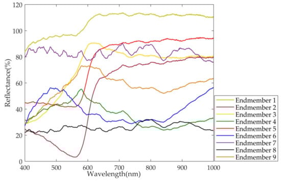
Figure 8.
Nine endmember spectral curves for the hyperspectral image of the Chinese painting.
Additionally, spectral matching was carried out between the endmember spectra and a pure pigment spectral library constructed by the laboratory. The spectral library contains more than 30 kinds of commonly used painting pigments of red, green, blue, yellow, black and white. The method of SFF, SAM and BE were combined to calculate the similarity between the unknown endmember spectral curves and standard pigment spectral curves. The fitting degree of the three methods was scored, and the final score was obtained with the weights of 0.5, 0.3 and 0.2, respectively. The higher the score, the higher the similarity between the two spectra. The top three spectral matching results and scores of each pigment are listed in Table 9.
Table 9.
The spectral matching and scores for nine endmembers.
Comparing the spectral matching results with the reference data, we found that the endmember of 1, 7, 9 could not be properly identified. It should be noted that the reflectance data of endmember 8 were low, while endmember 7 data were high. As the reflectance data of ink were relatively low, we think that endmember 8 was most likely to be the ink. The spectral matching results of endmember 2–6, 8 were consistent with the recorded pigments. The vermilion of endmember 5 was a synthetic pigment with the same composition as cinnabar. We used the highest similarity pigment as the type of endmembers. Therefore, we selected endmember 2–6, 8 to perform unmixing on the Chinese painting using the PPNM algorithm. The spatial abundance maps of each pigment are shown in Figure 9.
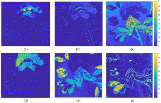
Figure 9.
Abundance maps of different pigment endmembers for the Chinese painting: (a) abundance map of eosin; (b) abundance map of orpiment; (c) abundance map of malachite; (d) abundance map of vermilion; (e) abundance map of azurite; (f) abundance map of ink.
As the painting was created based on traditional Chinese painting skills, it is hard to know the exact proportion of each pigment in each point of the hyperspectral image. However, the pigment maps in Figure 9 are basically consistent with the visual intensity of the image. Moreover, the abundance maps in Figure 9b–d,f displayed the spatial distribution of orpiment, malachite pigment, vermilion and ink. The PPNM could correctly unmix malachite from the mixture of ocher and malachite on part of the branches as shown in Figure 9c. However, for the abundance map of eosin shown in Figure 9a, it is hard to distinguish the pigments in the same color. There is an obvious abundance of eosin in the part of petals that was painted with the vermilion pigment. In the case of known endmember spectra, the PPNM could correctly be used to estimate the abundance of different pigments from the hyperspectral image of the Chinese painting.
5. Discussion
5.1. Unmixing Based on Continuum Removal Transformation of Reflectance Spectra
Continuum removal has already been utilized in nonlinear spectral unmixing due to its potential for eliminating nonlinear effects in spectral mixing [40]. The mixing of different mineral pigments tends to be more complicated, due to its component pigment of particle size, paint layer, etc. Therefore, we compared the accuracy abundance with and without continuum removal.
Continuum removal can highlight the absorption and reflectance characteristics of spectral curves, and normalize the reflectance between 0–1. It is modeled by Equation (14)
where is the normalized reflectance spectrum after continuum removal, is the measured reflectance spectrum, and is the spectral continuum, which is a convex hull fitted over the top of the spectrum.
In this study, we performed continuum removal on all measured spectra to study the nonlinearity of different pigment mixing and verify the effectiveness of continuum removal on the accuracy of abundance inversion. The reflectance spectra after continuum removal are shown in Figure 10.
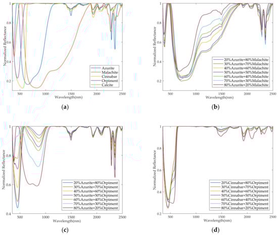
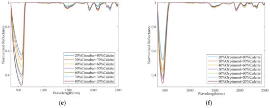
Figure 10.
Normalized reflectance spectra of pure pigments and mixed pigments with different mass ratios after continuum removal: (a) pure pigment normalized reflectance spectra; (b) the mixture of azurite and malachite normalized reflectance spectra; (c) the mixture of azurite and orpiment normalized reflectance spectra; (d) the mixture of cinnabar and orpiment normalized reflectance spectra; (e) the mixture of cinnabar and calcite normalized reflectance spectra; (f) the mixture of orpiment and calcite normalized reflectance spectra.
After performing continuum removal, the FCLS based on the linear mixing model as well as the FM, GBM, and PPNM based on the nonlinear mixing model, were carried out on the five groups of mixtures to obtain the abundances. For each mixture, the abundances of each pigment endmember and their RMSE values were calculated. To intuitively compare the abundance accuracy with and without continuum removal, the histograms of the RMSE values of the four algorithms are shown in Figure 11.
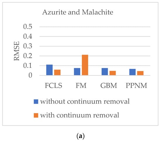
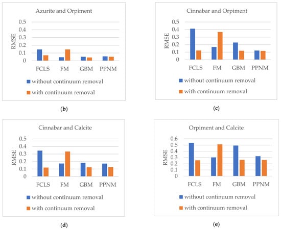
Figure 11.
The comparison of the RMSE values of four algorithms in different mixtures with and without continuum removal: (a) azurite and malachite; (b) azurite and orpiment; (c) cinnabar and orpiment; (d) cinnabar and calcite; (e) orpiment and calcite.
The following points can be seen from Figure 11. First, besides, the abundance accuracy of all the unmixing algorithms, except the FM, was improved on the five groups of samples. Second, the RMSE by the FCLS improved significantly with continuum removal. It was reduced to one-half or even one-third of the RMSE without continuum removal. Third, RMSE by the FCLS with continuum removal was close to that by the PPNM. For the mixture of cinnabar and calcite, shown in Figure 11d, the RMSE obtained by the FCLS with continuum removal was even better than that obtained by the PPNM. The reason for this may be that continuum removal is a kind of nonlinear transformation, so the nonlinear mixing effect of the reflectance spectrum for different pigments would be weakened to a certain extent after continuum removal. This again confirms the existence of the mixing nonlinearity and provides a way of combining it with the LMM to improve the unmixing accuracy through the NLMM in the pigment identification field.
5.2. Nonlinear Unmixing by the K-M Theory
The K-M theory has been successfully used to estimate the concentrations of the components in pigment mixtures. To compare the abundance accuracy obtained by the four above models with that obtained by the K-M theory, the single-constant K-M theory has been utilized for pigment unmixing.
In the case of pigment mixtures, according to the single-constant K-M theory, the of a mixture can be modeled as a linear combination of the of the component pigments. It can be given by Equation (15) [22]
where is the absorption coefficient, is the scattering coefficient and is the number of component pigments in a mixture ( in this study). and are the absorption and scattering coefficients of each component pigment, respectively. are their respective proportions. and are the absorption and scattering coefficients of the substrate.
In this study, we used raw rice paper as the substrate. Firstly, the reflectance spectra of pigment mixtures, pure pigment, and the rice paper were transformed into the . Secondly, we performed linear unmixing by the FCLS to estimate the abundances based on Equation (15). The abundances of the five groups of mixed pigment samples—azurite and malachite, azurite and orpiment, cinnabar and orpiment, cinnabar and calcite, orpiment and calcite—are listed in Table 10. Their RMSE values are also calculated.
Table 10.
Abundance estimated by the K-M theory for five groups of mixed pigment samples.
It can be seen in Table 10 that the abundances estimated by using and the FCLS after K-M transformation were not good, even worse than those estimated by using reflectance and the FCLS directly. Therefore, it is necessary to study the differences between pigments and seek a more suitable nonlinear unmixing method to identify the pigments on the surface of cultural relics.
6. Conclusions
An experimental approach was developed to investigate the nonlinear degree of reflectance spectra for the mixture samples formed from five commonly used mineral pigments, including azurite, malachite, cinnabar, orpiment, and calcite. The reflectance spectra of these samples were measured and unmixed by different algorithms based on the LMM and NLMM, respectively. The abundance accuracy of each pigment in the mixed samples by each algorithm was calculated by each algorithm. The similarity between the spectra measured by the instrument and that reconstructed by the unmixing results was also calculated. The accuracy and the similarity were employed together to evaluate the spectral nonlinearity of the pigment mixing. The following points can be concluded from the experimental results.
First, the abundance accuracies produced by the algorithms based on the NLMM were higher than those given by the algorithm based on the LMM for all samples, which indicates that the spectral mixing of mineral pigments is more in line with the nonlinear mixing model. On the other hand, the nonlinear degree of different pigments is different. The nonlinear mixing characteristics of the specific pigment should be considered when selecting an appropriate unmixing algorithm.
Second, the nonlinear mixing degree of the reflectance spectrum is related to the absorption/scattering coefficients and color of the component pigments in a mixture. For the five mineral pigments, the mixing spectral characteristics of the two pigments in a mixture were more linear, when the curves between them were significantly different. Otherwise, the mixing spectral characteristics of the two pigments in a mixture were more nonlinear, when the curves of them were similar or one of the pigments was white pigment. It is necessary to consider the nonlinear effect in these mixtures.
Third, the nonlinearity of pigment mixing is also related to the wavelength, which means that the degree of nonlinearity is different in different bands. The spectral nonlinearity of the mixed pigment was relatively high near the wavelength, corresponding to their colors. Meanwhile, the nonlinearity increased as the wavelength increased in the shortwave infrared bands, whose wavelength was greater than 1500 nm.
Fourth, as a kind of nonlinear transformation, continuum removal improved the accuracy of most discussed algorithms, especially the linear unmixing algorithm, because it could reduce the nonlinear degree of pigment mixing. However, it should be noted that the accuracy may be reduced for some nonlinear unmixing algorithms after continuum removal.
Finally, it should be noted that the results and conclusions are based on four unmixing algorithms, and the samples are each composed of two kinds of pigment. The experiments were conducted on the pigment mixtures with a single paint layer. The pigments mixing in multilayers is not discussed. We only carried out the pigment unmixing on a Chinese painting on raw rice paper. These topics are worthy of further study. However, the developed approach can provide useful ideas for exploring the spectral nonlinear characteristics of pigment mixtures.
Author Contributions
Conceptualization, S.L., D.M., and M.H.; methodology, S.L., and D.M.; validation, S.L., D.M., S.T., C.H., and J.M.; formal analysis, S.L., D.M., S.T., and C.H.; writing—original draft preparation and writing—review, all authors. All authors have read and agreed to the published version of the manuscript.
Funding
This research was funded by the National K&D Program of China (No. 2017YFB1402105), the Great Wall Scholars Training Program Project of Beijing Municipality Universities (No. CIT&TCD20180322), and an Independent Project of the Chinese Academy of Cultural Heritage (No. 2018JBKY13).
Conflicts of Interest
The authors declare no conflict of interest.
References
- Zhang, X. Chinese traditional pigment minerals. China Non-Met. Miner. Ind. Guide 2020, 4, 10–14. (In Chinese) [Google Scholar]
- Siddall, R. Mineral Pigments in Archaeology: Their Analysis and the Range of Available Materials. Minerals 2018, 8, 201. [Google Scholar] [CrossRef]
- Herens, E.; Defeyt, C.; Walter, P.; Strivay, D. Discovery of a woman portrait behind La Violoniste by Kees van Dongen through hyperspectral imaging. Herit. Sci. 2017, 5, 14. [Google Scholar] [CrossRef]
- Ma, C.; Liu, Z.; Cheng, L. Raman Spectra, XRF and SEM analysis of the pigments from the color paintings of Longmen Grottos. J. Light Scatt. 2018, 30, 357–361. (In Chinese) [Google Scholar]
- Howe, E.; Kaplan, E.; Newman, R.; Frantz, J.H.; Pearlstein, E.; Levinson, J.; Madden, O. The occurrence of a titanium dioxide/silica white pigment on wooden Andean qeros: A cultural and chronological marker. Herit. Sci. 2018, 6, 41. [Google Scholar] [CrossRef]
- Delaney, J.K.; Dooley, K.A.; van Loon, A.; Vandivere, A. Mapping the pigment distribution of Vermeer’s Girl with a Pearl Earring. Herit. Sci. 2020, 8, 4. [Google Scholar] [CrossRef]
- Gueli, A.; Gallo, S.; Pasquale, S. Optical and colorimetric characterization on binary mixtures prepared with coloured and white historical pigments. Dye. Pigment. 2018, 157, 342–350. [Google Scholar] [CrossRef]
- Shen, J.; Li, Y.; He, J. On the Kubelka-Munk absorption coefficient. Dye. Pigment. 2016, 127, 187–188. [Google Scholar] [CrossRef]
- Fonseca, B.; Patterson, C.S.; Ganio, M.; MacLennan, D.; Trentelman, K. Seeing red: Towards an improved protocol for the identification of madder-and cochineal-based pigments by fiber optics reflectance spectroscopy (FORS). Herit. Sci. 2019, 7, 92. [Google Scholar] [CrossRef]
- Grabowski, B.; Masarczyk, W.; Głomb, P.; Mendys, A. Automatic pigment identification from hyperspectral data. J. Cult. Herit. 2018, 31, 1–12. [Google Scholar] [CrossRef]
- Wang, L.; Li, Z.; Ma, Q.; Mei, J. Non-destructive and in-situ identification of pigments in wall paintings using hyperspectral technology. Dunhuang Res. 2015, 3, 122–128. (In Chinese) [Google Scholar]
- Wu, T.; Li, G.; Yang, Z.; Zhang, H.; Lei, Y.; Wang, N.; Zhang, L. Shortwave infrared imaging spectroscopy for analysis of ancient paintings. Appl. Spectrosc. 2016, 71, 977–987. [Google Scholar] [CrossRef]
- Li, J.; Wan, X. Superpixel segmentation and pigment identification of colored relics based on visible spectral image. Spectrochim. Acta Part A Mol. Biomol. Spectrosc. 2017, 189, 275–281. [Google Scholar] [CrossRef]
- Chen, J.; Richard, C.; Honeine, P. Nonlinear unmixing of hyperspectral data based on a linear-mixture/nonlinear-fluctuation model. IEEE Trans. Signal. Process. 2013, 61, 480–492. [Google Scholar] [CrossRef]
- Deborah, H.; George, S.; Hardeberg, J.Y. Pigment mapping of the scream (1893) based on hyperspectral imaging. In Proceedings of International Conference on Image and Signal Processing; Springer: Berlin/Heidelberg, Germany, 2014; Volume 8509, pp. 247–256. [Google Scholar]
- Bai, D.; Messinger, D.W.; Howell, D. A hyperspectral imaging spectral unmixing and classification approach to pigment mapping in the Gough & Selden Maps. J. Am. Inst. Conserv. 2019, 58, 69–89. [Google Scholar]
- Zhao, H.; Zhang, L.; Wu, T.; Huang, C. Research on the model of spectral unmixing for minerals based on derivative of ratio spectroscopy. Spectrosc. Spectr. Anal. 2013, 33, 172–176. (In Chinese) [Google Scholar]
- Lyu, S.; Liu, Y.; Hou, M.; Yin, Q.; Wu, W.; Yan, X. Quantitative analysis of mixed pigments for Chinese paintings using the improved method of ratio spectra derivative spectrophotometry based on mode. Herit. Sci. 2020, 8, 31. [Google Scholar] [CrossRef]
- Wang, G.; Liu, Z. Mixed pigment composition analysis method based on spectral representation and independent component analysis. Spectrosc. Spectr. Anal. 2015, 35, 1682–1689. (In Chinese) [Google Scholar]
- Rohani, N.; Salvant, J.; Bahaadini, S.; Cossairt, O.; Walton, M.; Katsaggelos, A. Automatic pigment identification on Roman Egyptian paintings by using sparse modeling of hyperspectral images. In Proceedings of 2016 24th European Signal Processing Conference (EUSIPCO), Budapest, Hungary, 29 August–2 September 2016; IEEE: Budapest, Hungary, 2016; pp. 2111–2115. [Google Scholar]
- Kubelka, P.; Munk, F. An article on optics of paint layers. Z. Tech. Phys. 1931, 12, 259–274. [Google Scholar]
- Taufique, A.M.N.; Messinger, D.W. Hyperspectral pigment analysis of cultural heritage artifacts using the opaque form of Kubelka-Munk theory. In Proceedings of Algorithms, Technologies, and Applications for Multispectral and Hyperspectral Imagery XXV; SPIE Defense + Commercial Sensing: Baltimore, MD, USA, 2019; p. 1098611. [Google Scholar]
- Rohani, N.; Pouyet, E.; Walton, M.; Cossairt, O.; Katsaggelos, A.K. Nonlinear unmixing of hyperspectral datasets for the study of painted works of art. Angew. Chem. 2018, 130, 11076–11080. [Google Scholar] [CrossRef]
- Bai, D. A Hyperspectral Image Classification Approach to Pigment Mapping of Historical Artifacts Using Deep Learning Methods; Rochester Institute of Technology: Rochester, NY, USA, 2019. [Google Scholar]
- Kleynhans, T.; Schmidt Patterson, C.M.; Dooley, K.A.; Messinger, D.W.; Delaney, J.K. An alternative approach to mapping pigments in paintings with hyperspectral reflectance image cubes using artificial intelligence. Herit. Sci. 2020, 8, 84. [Google Scholar] [CrossRef]
- Zhang, S.; Fu, Q.; Yang, L.; Ma, Y.; Wang, W.; Zhang, W.; Zhang, J.; Fang, X. Research on polychrome and binding media of acrobat figures in pit K9901 of Qinling. Sci. Conserv. Archaeol. 2020, 4, 82–88. (In Chinese) [Google Scholar]
- Li, Y.; Zhao, L.; Fang, X.; Wang, L. Characterization and properties of gelatin as a kind of conservation material for painted cultural relics. J. Northwest. Norm. Univ. Nat. Sci. 2021, 1, 70–76+83. (In Chinese) [Google Scholar]
- Zhao, Y.; Berns, R.S.; Taplin, L.A.; Coddington, J. An investigation of multispectral imaging for the mapping of pigments in paintings. In Proceedings of Computer Image Analysis in the Study of Art; SPIE: New York, NY, USA, 2008; Volume 6810, p. 681007. [Google Scholar]
- Bioucas-Dias, J.M.; Plaza, A.; Dobigeon, N.; Parente, M.; Du, Q.; Gader, P.; Chanussot, J. Hyperspectral unmixing overview: Geometrical, statistical, and sparse regression-based approaches. IEEE J. Sel. Top. Appl. Earth Obs. Remote Sens. 2012, 5, 354–379. [Google Scholar] [CrossRef]
- Heinz, D.C.; Chang, C.I. Fully constrained least squares linear spectral mixture analysis method for material quantification in hyperspectral imagery. IEEE Trans. Geosci. Remote Sens. 2001, 39, 529–545. [Google Scholar] [CrossRef]
- Altmann, Y.; Dobigeon, N.; Tourneret, J.-Y. Bilinear models for nonlinear unmixing of hyperspectral images. In Proceedings of 2011 3rd Workshop on Hyperspectral Image and Signal Processing: Evolution in Remote Sensing (WHISPERS); IEEE: Lisbon, Portugal, 2011; pp. 1–4. [Google Scholar]
- Fan, W.; Hu, B.; Miller, J.; Li, M. Comparative study between a new nonlinear model and common linear model for analyzing laboratory simulated-forest hyperspectral data. Int. J. Remote Sens. 2009, 30, 2951–2962. [Google Scholar] [CrossRef]
- Heylen, B.; Scheunders, P. A Multilinear mixing model for nonlinear spectral unmixing. IEEE Trans. Geosci. Remote Sens. 2015, 54, 1–12. [Google Scholar] [CrossRef]
- Halimi, A.; Altmann, Y.; Dobigeon, N.; Tourneret, J.-Y. Unmixing hyperspectral images using the generalized bilinear model. In Proceedings of 2011 IEEE International Geoscience and Remote Sensing Symposium; IEEE: Vancouver, BC, Canada, 2011; pp. 1886–1889. [Google Scholar]
- Altmann, Y.; Halimi, A.; Dobigeon, N.; Tourneret, J.-Y. Supervised nonlinear spectral unmixing using a postnonlinear mixing model for hyperspectral imagery. IEEE Trans. Image Process. 2012, 21, 3017–3025. [Google Scholar] [CrossRef]
- Dobigeon, N.; Tits, L.; Somers, B.; Altmann, Y.; Coppin, P. A comparison of nonlinear mixing models for vegetated areas using simulated and real hyperspectral data. IEEE J. Sel. Top. Appl. Earth Obs. Remote Sens. 2014, 7, 1869–1878. [Google Scholar] [CrossRef]
- Meng, D.; Lv, S.; Hou, M.; Gao, Z. On geometry-simplex endmember extraction algorithms for the mixed pixel of typical mineral pigment mixture. Geomat. World 2020, 27, 1–6. (In Chinese) [Google Scholar]
- Zhao, H.; Zhao, X.; Liu, X. Spectral mixing model of mineral pigments on Chinese paintings-taking cinnabar and orpiment for example. Sci. Technol. Eng. 2018, 18, 6–11. (In Chinese) [Google Scholar]
- Ren, H.; Chang, C.I. Automatic spectral target recognition in hyperspectral imagery. IEEE Trans. Aerosp. Electron. Syst. 2003, 39, 1232–1249. [Google Scholar]
- Zhao, H.; Zhao, X. Nonlinear unmixing of minerals based on the log and continuum removal model. Eur. J. Remote Sens. 2019, 52, 277–293. [Google Scholar] [CrossRef]


Publisher’s Note: MDPI stays neutral with regard to jurisdictional claims in published maps and institutional affiliations. |
© 2021 by the authors. Licensee MDPI, Basel, Switzerland. This article is an open access article distributed under the terms and conditions of the Creative Commons Attribution (CC BY) license (https://creativecommons.org/licenses/by/4.0/).