
Modelling Large Heaped Fill Stockpiles Using FMS Data


Department of Mining Engineering, University of Utah, Salt Lake City, UT 84112, USA
*
Author to whom correspondence should be addressed.
Minerals 2021, 11(6), 636; https://doi.org/10.3390/min11060636
Submission received: 21 April 2021
/
Revised: 5 June 2021
/
Accepted: 8 June 2021
/
Published: 15 June 2021
(This article belongs to the Special Issue Advances in Computational Intelligence Applications in the Mining Industry)
Abstract
:The frequent best practice for managing large low-grade run-of-mine (ROM) stockpiles is to average the entire stockpile to only one grade. Modern ore control and mineral processing procedures need better precision. Low-precision models hinder the ability to create a digital mine-to-mill model and optimize the holistic mining process. Prior to processing, poorly characterized stockpiles are often drilled and sampled, despite there being no geological reason for relationships between samples to exist. Stockpile management is also influenced by reserve accounting and lacks a common operational workflow. This paper provides a review of base and precious metal run-of-mine (ROM) pre-crusher stockpiles in the mining industry, and demonstrates how to build a spatial model of a large long-term stockpile using fleet management system (FMS) data and geostatistical code in Python and R Studio. We demonstrate a framework for modelling a stockpile believed to be readily workable for most modern mines through use of established geostatistical modelling techniques applied to the type of data generated in a FMS. In the method presented, each bench of the stockpile is modeled as its own geological domain. Size of dump loads is assumed to contain the same volume of material and grade values that match those of the grade data tracked in the FMS. Despite the limitations of these inputs, existing interpolation techniques can lead to increased understanding of the grade distribution within stockpiles. Using the framework demonstrated in this paper, engineers and stockpile managers will be able to leverage operational data into valuable insight for empowered decision making and smoother operations.
1. Introduction
1.1. Objective
As mines are depleted and average global ore grades decline, the desire for an improved working model for stockpile management is likely to grow [1]. Fortunately, digitization efforts have increased throughout the mining industry in recent years, and there is already pressure for mining companies to make use of their new data [2]. Stockpiles are composed of not just valuable material, but also valuable and often misunderstood data, which makes them prime targets for the benefits of digital innovation [3]. This paper provides a review of base and precious metal run-of-mine (ROM) pre-crusher stockpiles in the mining industry, and demonstrates how to build a spatial model of a large long-term stockpile using fleet management system (FMS) data and geostatistical code in Python and R Studio.
1.2. Background
Early base and precious metal mining endeavored to extract the richest ores available. In this scenario, miners would send rich ore directly to milling facilities. With the advent of industrial mining during the 19th century, partly due to Watt and the steam engine [4], mines scaled up into large tonnage operations capable of processing large tonnages of ore. For the first time, low-grade ores could be mined profitably [5]. As a result of these larger mines, the need for stockpiling gradually grew until they were justified to be economically advantageous over the course of a mine life [6,7,8].
According to Yi [7], the initial work around cut-off grades began in the 1960s and incorporated stockpiles in the 1980s [9]. These works determined that a stockpile will be required for any case in which a mine plans to change cut-off grade over the course of its life. Presently, the stockpiling of ore has become an integral part of mine planning [10,11]. Effective mine planning requires a detailed understanding of the ore deposit. This understanding is then leveraged into a production strategy that considers both the current mining environment as well as predictions of future demand, commodity prices, and other conditions.
Much work has been carried out to determine when base and precious metal mines should stockpile (cut-off grades, net present value (NPV) calculations, rehandle costs, milling costs, production contracts, mine planning, etc.) [1,11,12,13,14,15,16,17]. The discipline of managing stockpiles throughout mining operations to maximize the profit gained from their eventual processing is still emerging [18]. Often stockpiles are created as an afterthought or side effect to increased production. Occasionally, they are inherited from previous operators upon the purchase of a mine [19]. In some operations, stockpiles are required to fit into a space confined to a permit area they were not originally intended for.
The use of stockpiles has become paramount to the economic viability of production strategies for several reasons, which include the following:
1.3. Classification of Stockpiles
As is the case with many processes, blending or mixing is a necessary step to ensure optimal product quality. Typically, these blending processes are performed after the primary crusher step. Within mining, pre-crusher stockpiling is often used for its operational simplicity, but it typically lowers the confidence of the ore grade and reduces certainty in feed quality [15]. Pre-crusher stockpiling takes on five forms which are illustrated in Figure 1 [15,16,17]:
Just as there are operational differences between iron, coal and base and precious metal mining, there are also differences in how these operations stockpile. For example, iron ore is often shipped directly from the mine to the customer. Since the tonnages involved are immense, extensive work has already been carried out to model the way that iron ore should be stockpiled for re-handle [16,17,24,25]. Likewise, due to hazards around coal (loss of energy through oxidation, spontaneous combustion, etc.) and since it is typically directly shipped, there has been much work dedicated to understanding how it behaves during stockpiling [26].
For large-scale base and precious metal mine stockpiles, however, little scientific literature exists to document how to spatially model multivariate distribution of characteristics such as grade, hardness, rock type, and other geochemical properties. Kasmaee et al. [27] demonstrated a method using sampling from the base of stockpiles in conjunction with monthly surveying to create a kriging of an iron ore stockpile in Iran. Morley and Arvidson [28] mention that stockpile modelling typically involves arithmetic weighted averages of grade and tonnage values determined from blast hole samples and survey volume records. They also state that spatial modelling of stockpiles is performed manually using engineering software tools. The disadvantage of these manual models is that they require constant engineering resources which could be spent elsewhere. They are also subject to human error, risk of employee turnover and inconsistencies in their design method. Furthermore, base and precious metal stockpiles are classified as temporary storage [29] and their contents shift over time. Dozers and other heavy equipment frequently displace stockpiled material from its original dump location, making it hard to know where material is located within the stockpile.
Another way of classifying stockpiles is by their construction design. Figure 2 shows the different types of stockpile constructions which are common in mining operations.
According to Carter, solutions for stockpile management are built into roughly a dozen comprehensive mine scheduling software platforms [18]. These software systems integrate with short-term and small-scale stockpiles, but they do not serve well for large, long-term, truck-dumped stockpiles. Generally, the stockpile modelling software that exists is tailored to conveyor systems for intermediate stockpiles [24,25], but it may be possible to apply some of their concepts to larger stockpiles. Discrete element modelling (DEM) [30] has demonstrated the ability to model material flow of intermediate stockpiles, but remains unproven for large stockpiles where particles are exceedingly numerous and variable.
In addition to modelling, documented technical methods for tracking ROM ore from haul trucks into large stockpiles and onward through downstream processes are perfunctory. Surface base and precious metal mines typically use global positioning systems (GPS) to track haul truck movement and fleet management systems (FMS) to optimize productivity. Afrapoli and Askari-Nasab [31] provide a detailed and current review of FMS technology. FMS systems perform best for tracking material directly dumped from pit to crusher, but lack the capability to track ore once it has been dumped into a stockpile.
Material tracking technology exists, but is rarely used in large stockpiles due to the long duration of time from the placement of the ore to processing. Jansen et al. [32] demonstrated proof of concept case studies involving SmartTag™ radio-frequency identification (RFID) tracer technology for both source-to-product as well as process hold-up ore tracking for the Northparkes mines in Australia. Jurdziak et al. [33] discuss the challenges, propose a workflow and estimate savings of 2.5 million euros for implementing RFID ore tracking at the KGHM Lubin mine in Poland. In addition to RFID, unmanned aerial vehicle (UAV) technology, while promising for its ability to determine stockpile volumes [34,35], is still incipient for the purposes of predicting grade distribution within the stockpile or tracking material movement.
Failing to adequately track and model ore stockpiles results in a loss of data already gained from geological exploration and mine production as illustrated in Figure 3. Such a failure represents not only data and money wasted, but also an opportunity lost in saving additional money during the processing of the stockpiled materials. This is a double lost opportunity for the operator who is probably already operating on relatively thin margins.
Figure 3 illustrates a conceptual loss of data associated with stockpiled material that was previously available from exploration models and operational logs. Moreover, the figure illustrates how information is added about the material at each processing step, including production drill sample analyses, ore control modelling and fleet management system information, until the time of stockpiling. Data from each of these operational steps potentially add value to the material if appropriately used, but it is also wasted if the material is not tracked into the stockpile.
If a modern mine can be considered as a digital system of production, stockpiles may be thought of as digital bottlenecks, since they output less information into downstream processes than was input into them [36]. According to Kahraman et al. [37], identifying, tracking, and managing bottlenecks will enable significant improvement in mining operations. However, data gaps, such as stockpiles, short circuit the bottleneck tracking capabilities of sites not to mention, automation, mine-to-mill, and other operational improvement initiatives. While missing data can be thrown out to little detriment for estimation purposes (grade, tonnage, amount of explosive needed, etc.), they need to be included for predictive purposes (capital asset performance, maintenance, throughput, mine-to-mill, etc.) [38].
1.4. Reconciliation and Metallurgical Accounting
Despite little documentation on technical modelling methods, literature contains robust discussion on stockpiles as they pertain to reconciliation and metal accounting [32]. After the Sarbanes-Oxley Act of 2002 [39], the requirement for real-time disclosure of financial conditions to stakeholders in the mining business has inspired more systematic approaches to reconciliation and therefore more scrutiny of stockpiles. Macfarlane [40] contends that a full understanding of metal flow is necessary in order for there to be a systematic approach to reconciliation. Random stockpiling without a clearly defined process map can make accounting for tonnage discrepancies futile. Misunderstanding of stockpile characteristics reduces conversion of mineral resource inventory into saleable product. Motivations for stockpile misunderstandings, underappreciation and neglect are numerous, but generally include issues from the following categories [40,41]:
- Sampling accuracy,
- Data recording and material tracking,
- Geological modelling and estimation errors,
- Short-term and intermediary stockpile accounting,
- Mine design and mine planning,
- Grade control,
- Dispatch,
- Survey inconsistencies,
- Interdepartmental communication,
- Mine operations,
- Management,
- Training and turnover of employees, and
- Dilution, natural leaching and other factors.
Ghorbani and Nwalia [41] affirm that mass flow measurement, stream sampling, mass balancing, and data handling and reporting are the four components of metallurgical accounting. Large, long-term stockpiles pose challenges to each of these components. Stockpiles are difficult to measure and sample [28]. They also risk being manipulated for the purposes of balancing the overall deposit metal value, may become orphaned by multiple operational departments and offer low incentives to be accurately recorded or reported on a frequent basis [41,42]. Improvements in technical capacity to model and manage stockpiles will therefore benefit reconciliation and metallurgical accounting. However, these technical improvements must be incorporated into mining workflows for such benefits to be reaped. Fortunately, existing reserve and operational models provide a foundation for the incorporation of a stockpile working model.
1.5. Reserve and Operational Models
The primary method currently used to model stockpile characteristics in mining is averaging the materials stockpiled and reconciling the values against reserve and operational models. Figure 4 illustrates key aspects of reserve and operational models. A reserve model accounts for the entire life of mining operations and is based primarily on exploration drill holes that are widely spaced apart compared to production drilling. This model is updated biannually and contains more risk and uncertainty than the other models. Short term operational models are a type of hybrid between ore control models and the reserve model and are used for the purposes of planning on a one-to-three-year time horizon. Ore control models are made from additional data obtained by production drilling and contain only the information pertinent to areas of immediate mining within the next week to month for operational purposes. While some details vary in the drillhole spacing and the amount of hybridization between the short-term model, the reserve model and the ore control model, most mining operations follow some version of this established working model.
Unlike the reserve and operational models described previously, to the knowledge of the authors, there is no documented working model for large long-term stockpile characteristic distribution, which poses some issues. First, since stockpiles are not income-generating assets, without a working model that is easily implemented, they typically suffer neglect. Moreover, since many short-term discrepancies in ore reserve accounting can be written-off over time under the guise of environmental degradation [42] of stockpiles at the end of the mine life, the absence of a working model may be a disincentive to dedicate engineering resources to their concurrent management. Ultimately, these practices reduce confidence in the characteristics of stockpiled material and lead to a wasteful duplication of time and energy in drilling, and sampling, when the stockpile is finally set to be processed. Many stockpile working models have been developed manually by mining engineers to meet industry needs. However, there is a knowledge gap between the practical methods developed within industry and scientific documentation.
1.6. Sampling
Many sampling issues have been identified to exist for both stockpiles as well as ore control operational models. In the case of ore control, blast hole sampling from drill collars has undergone intense scrutiny from the sampling community. Engström [43] provides a recent literature review on this scrutiny and states that blast hole sampling problems include loss of fines (or inaccurate particle size distribution representation), upward/downward contamination, influx of sub-drill material, pile segregation, pile shape irregularities, operator-dependent sampling, too small sample size, frozen (or weathered) blast hole cones and non-equiprobabilistic sampling equipment. Further complications to ore control understanding exist due to material movement after blasting. Thornton [44] states that material moves more than 4 m on average and movements of 10 m are common. Depending on the drill pattern, this movement could equate to a displacement from the initial sample location to up to three sample locations away.
The probability of a misclassification of ore to waste or waste to ore from sampling errors alone is commonly between 5% and 20% for base and precious metal mines [45,46]. In addition, ore loss of 9% to 19% due to blast movement and dilution can be expected [44]. The negative impacts of these issues may become more critical when handling precious metals and FMS data do not typically contain adjustments for them. However, the problem of data accuracy is separate from that of data utilization. If FMS data are used more frequently for modelling, then improvements in data accuracy will be encouraged through data feedback loops. Improvements in sensor technology could lead to increased sampling of mining operations and eventually better account for blast movement, dilution and sampling errors. It is probable that incorporating these more accurate measuring methods may help to improve the precision of the entire approach.
1.7. Current Practice and Scope
Industry sources have revealed that current practice is to take a running average of the material characteristics that are fed into the stockpile over time. These running averages are based on the reconciled survey volumes and grade values of materials and are updated concurrent with reserve and operating models. This process is designed to fulfill legal reporting requirements. Despite there being a large amount of data that are tracked in the FMS, the resulting stockpile block model currently in place is merely one large, homogenized block value containing the rolling average grade.
At this time, it is the understanding of the authors that no documented methodology exists in academic literature for determining the grade distribution of large, low-grade, randomly truck-dumped, pre-crusher stockpiles via FMS data. In such cases, drilling and grab sampling of the stockpile are often performed in order to determine the grade distribution and model the stockpile. These techniques have proven to be erroneous and biased [28]. We therefore present and explore an initial approach believed to be readily workable for most modern mines through use of established geostatistical modelling techniques applied to the type of data generated by FMS. This method is part of an ongoing study into developing an engineering methodology for greater understanding of large ROM truck-dumped stockpiles.
The working model for stockpile management conceived in this paper can attenuate the negative impacts of the present stockpiling scenario. It requires minimal engineering resources, is easy to setup and maintain over a long period of time, makes use of readily available data already existing in most modern mines and yields a high amount of detail. Our method could be used as a stand-alone model, or it could be used to enhance or verify other models. This method is software agnostic and can be integrated with mining software packages, as we will demonstrate.
2. Materials and Methods
2.1. Approach
A data-driven approach was used to develop a working model of the characteristics of the stockpile. This approach combined the knowledge of the mine planners with that of the researchers in a process similar to the one demonstrated by Subramaniyan et al. [47]. For the purposes of this paper, as it is an example of the modelling technique, the exact data presented are not real data but exemplify real data seen by researchers and demonstrate a hypothetical stockpile created to show the design method. Figure 5 outlines the methodology used.
As demonstrated in Figure 5, the inputs of the mine planners were used during each step of model development. In Step 1 mine planners shared relevant data with researchers, helped clarify questions about the data itself along with explaining any outliers and also defined the project boundary while researchers explored and cleaned the data. During Step 2 researchers presented some early visualizations of the raw data and prepared the modelling concepts. Mine planners provided feedback and context for the data visualization. Step 3 involved preparing and refining the model in accordance with mine planner requirements. Step 4 consisted of a final analysis and review. Each step provides the opportunity for feedback to prior and subsequent steps in the process for the purposes of tuning the final model.
2.2. Data
For the actual case study, a variety of survey, FMS, geological look-up tables, design files, and drone photogrammetry data were made available to the research team. These data have been kept proprietary and this paper contains only a hypothetical stockpile created in likeness of the real data. The flow of data used for creating the model for the actual case study is shown in Figure 6.
FMS data came from the mines dispatching system, which contained information about trucks, grade IDs (ore control patterns), dumping locations, dump tonnage, and dumping coordinates. Assay table data contained grade values along with other details about the material such as hardness, rock type, concentration of deleterious elements, etc. Assay table data were matched to corresponding grade IDs in the FMS data. These values were interpolated into a block model by the same method demonstrated subsequently in this paper. Survey data consisted of .dxf files from survey pickups. Survey data were used to create the topographical extents of the block model and ensure that blocks were sequenced correctly. Historical surveys were used to verify that interpolated block values existed matched the real time frame.
A hypothetical dataset was made to illustrate the design method in this paper without revealing the proprietary data of the site. Table 1 and Table 2 describe this hypothetical dataset, which represents the results of the combined FMS and assay table data shown in Figure 6. These data are statistically similar to the data used at the case study location and are similar to operational data available to most modern mines. The hypothetical example is that of an open pit gold mine, but the methodology could easily be applied to any other base or precious metal mine.
As this model is a hypothetical example, survey volumes were designed in Maptek Vulcan for the creation of the stockpile survey data. Maptek Vulcan was chosen only because it was familiar and accessible to both the research team and the mine involved in the study. The model is software agnostic and compatible with any engineering software which uses .dxf file format. Other file formats may also prove compatible with the model in the future. The dimensions of the hypothetical heaped fill stockpile are 150 m × 150 m × 5 m. Figure 7 shows a screenshot of the designed hypothetical stockpile.
Since the accuracy of each elevation value was limited to the value of the bench level, each bench was modeled as a two-dimensional plane. In the actual case study, each bench was aggregated to create the final block model. For the example shown in this paper, only one bench is demonstrated. While there is some difference in the tonnage values of each truck load in the data, for the purposes of this model, all dump locations were assumed to contain the same amount of material. Only one bench is demonstrated in this paper, but by this method multiple benches can be modelled as independent domains and combined into a block model for an entire stockpile.
2.3. Model
The block model was computed using R scripts running on a Python Jupyter Notebook Kernel. This notebook was developed using concepts from Pyrcz [48]. First, the combined values given by the FMS and assay data were imported into a dataframe. Then, the bench height given by the dump location was converted into an elevation or Z value for each of the dump coordinates. A dataframe consisting of the centroid locations for each block in the desired block model extents was then created. Finally, values for the block centroids were interpolated from the initial dataframe and assigned based on the inverse distance weighting (IDW) function from the gstats package in the R programming language to the centroids of the dataframe representing the block model. These centroids were then imported into Maptek Vulcan to demonstrate the capability of the model to be made useable by an engineering team.
The gstats package, developed by Edzer Pebesma [49], in the R programming language performs a number of common geostatistical functions. Pebesma outlines the modelling approach which should be used with gstats which is shown as Figure 8.
Inverse distance weighting (IDW) was selected as the modelling method in accordance with Figure 8, in that prediction locations were specified while variograms and base functions were not. Within gstats, the IDW function works the same way as the ordinary kriging function only without a model being passed and instead the inverse distance weighting power is directly specified by the user (β = 2) (see Equation (1)). A global search neighborhood (default parameter) was used for the model, meaning that all data points were used for estimating the value at each location.
IDW is a form of interpolation. Interpolation means to predict an attribute value ẑ from sampled locations xi at unsampled sites (x0) of a given neighborhood [50]. In this case, each of the dump locations along with corresponding grade values (ẑ) were considered as the “sampled locations” (xi) and the unsampled sites (x0) were an array of block model centroid values (x and y coordinates within the model space at 15 m × 15 m spacings). While the general IDW equation varies slightly [51], for the purposes of the model shown in this paper, the equation used for interpolation is
where Zx,y is the centroid point to be estimated, n is the number of samples, zi represents the value of the ith sample, dx,y,i is the distance between Zx,y and zi, and β is the user specified weight value.
This paper does not address which geostatistical method is best suited for modelling stockpiles. It is meant to demonstrate that FMS data are capable of being used along with geostatistical methods for greater operational understanding of stockpile characteristics. IDW was selected to show that FMS data are amicable to such methods of interpolation commonly employed in geostatistics. It was also chosen because it runs quickly without requiring additional model parameters as an input, whereas variogram modelling is more time consuming and does not create a block model as a final product. The discussion section of this paper includes more information on how to further refine the initial model.
3. Results
In a heaped fill stockpiling scenario, dumping occurs in two phases. The first phase is a series of paddock dumps to form the base layer of the stockpile. The second phase involves building an upper layer above an area of the paddock dumps from which a campaign of edge dumps occurs until the bench is completed. Our results are broken down into the scenarios described, being first paddock dumping, second edge dumping and third a look at both in combination.
3.1. Data Visualization
Figure 9 shows an initial visualization of the hypothetical dataset. In Figure 9 each dot represents a single dump of similar volume. The positions of the dots represent the FMS tracked dumping position of the truck at the time of dumping. The dot colors represent the interval of their grade values in accordance with the legend shown.
Visualizing FMS data in this manner allows for the identification of some areas of homogeneity within the stockpile. One area would be the bottom left part of the figure, where many black dots are near each other. It also reveals that most of the stockpile contains areas of mixed values and it is not easily visually interpreted into a workable model.
The data from Figure 9 can be broken down into two types of data for greater understanding and better modelling. Each of the data types refer directly to the dumping process used to create the data. The first type of data is termed base layer or paddock dumping data and refers to instances in the data where the material was dumped as a heap on a roughly flat surface. The second type of data is called upper layer or edge dumping data and refers to situations where material was dumped down an existing stockpile face. Each of these data types were also explored and modeled.
3.2. Base Layer/Paddock Dumping Model
Via preliminary data analysis, FMS data which corresponds to paddock dumps and forms the base layer of a stockpile in a hypothetical scenario are shown in Figure 10. In Figure 10 each dot represents a single dump of similar volume. The positions of the dots represent the FMS tracked dumping position of the truck at the time of dumping. The dot colors represent the interval of their grade values in accordance with the legend shown.
As is the case with paddock dumping for the base layer of a stockpile, the rows space evenly and maintain homogeneity along their respective row or column as the material originated from various low-grade areas in the pit of different grade amounts. This scenario occurs at the beginning of each bench of the stockpile or from paddock dumping areas where no upper layer is added. Material dumped this way is only handled by dozers or other heavy equipment in areas around the perimeter of the stockpile. Areas where dumps occurred too close to one another tend to settle into more vacant areas over time.
In the paddock dumping scenario, the area of influence of each truck load is closely related to the dimensions of the haul truck used. Figure 11 illustrates how truck dimensions influence the size and shape of the dumped material.
From Figure 11, the resulting heap of material takes on geometric form similar to that of an elliptical frustum. The height, length and width (H, W, L in Figure 11) of the heap are dependent on the respective height, width and length of the haul truck used. These dimensions may be extended in horizontal directions if the haul truck moves excessively during the dumping of its material, which will also coincide with a reduction in the height of the corresponding heap. The width may also expand beyond the original width of the truck if the truck does not move forward. A movement of less than two meters during dumping is a common occurrence and this movement typically only affects the length of the heap, not the width. Movements occur most frequently when a truck has backed up too close to the neighboring heap before beginning its dumping phase, which acts to smooth out the overall average area of influence of multiple paddock dumps for a given area. At the time of dumping, heaps maintain an approximate 2:1 slope, consistent with that of heaped loaded material. Over time the slope decreases to that of the natural angle of repose of the material.
Figure 10 alone is sufficient to create a working model for a paddock-dumped stockpile without the need of additional modelling. If operators have an approximate understanding of where heaps of given ore values are located, they can easily match those locations to the corresponding heaps during operation. Blending the example shown in Figure 10 can be intuitively performed by processing the stockpile in parallel vertical approaches as needed.
3.3. Upper Layer/Edge Dumping Model
Figure 12 shows hypothetical FMS data for the second phase of heaped fill stockpile construction. Like Figure 10, each dot in Figure 12 represents a single dump of similar volume. The positions of the dots represent their FMS tracked position. The dot colors represent the interval of their grade values in accordance with the legend shown. During this phase, material is dumped on top of the material of the base layer. However, data from the previous layer have been removed to facilitate visualization.
Figure 12 demonstrates that many dumping locations are clustered together in the initial area where the upper layer of the stockpile is first made (top left of Figure 12). Afterwards, the stockpile is built by edge dumping material from the initial dumping area until it fills the designed volume for the given bench. Dozers and other heavy equipment help to ensure that material is cascaded without clumping, ensure compaction and maintain safety berms during operation. These actions mix the material from its initial dumping location in intractable ways.
While the FMS data in the previous phase could be defined by orderly row and column behavior, within this upper layer, the dumping process is defined by radial progression from an initial cluster point. Variation in the grade distribution is therefore defined by the tendency of the material to be added in sweeping radial movements which correlate with low-grade patterns of various grades in the pit.
Generally, its assumed that the volume of influence for of the haul truck in the upper layer/edge dump case is that of dimensions in width equal to the width of the haul truck, length equal to the horizontal component of the bench slope and variable height which is influenced by width, length and material characteristics. This volume runs perpendicular to the tangent of the dump location and is illustrated in Figure 13.
While the total volume of material is influenced by the capacity of the haul truck, during this phase the shape of the material dumped is mostly influenced by bench height and material characteristics. When edge dumping occurs normally, that is without rehandling from dozers or other equipment, the resulting shape is a streak of material cascaded along the entire face of the stockpile. This cascade of material typically aggregates more at the bottom of the dumping area under normal conditions and less near the top crest of the dump. Depending on the face of the stockpile larger amounts of material may clump at various places along the face. Round and large material may also roll beyond the floor of the bench, especially at higher bench heights. The authors recognize that these are initial assumptions and more discussion on improvement of the model may be found in the discussion section of this paper.
It should be noted that paddock dumping still occurs on top of the dump area during the edge dumping phase. These dumps are usually to patch and level the floor of the dump area, create safety berms or protect light stations. Occasionally, paddock dumping occurs near the edge before subsequentially being pushed over by a dozer. Operator error may cause trucks to misalign with the edge of the dump creating a more turbulent cascade. Such dumping scenarios are extremely difficult to identify from the data alone.
While it does not offer an operational model on its own, Figure 12 still serves as a starting point. Most homogeneity occurs in radial/diagonal left-to-right directions and at the corners. As with Figure 10, optimizing stockpile processing can intuitively follow the observable pattern of homogeneity (bottom left to top right or vice versa). Unlike Figure 10, operators will have a harder time identifying which area corresponds to which heap shown in the data. This scenario also contains more natural mixing of material due to settling and dozer handling than does the previous scenario.
3.4. Interpolation Model
Unlike Figure 10 and Figure 12, Figure 9 offers no visual foundation for an operational model. The approach considered for such a situation is that of interpolation. Figure 14 shows an example of an interpolated model for the hypothetical stockpile using the inverse distance weighting method described in the method section. In this scenario, the area of influence of each truck load is difficult to determine since material that was dumped first affects the form that material dumped later takes.
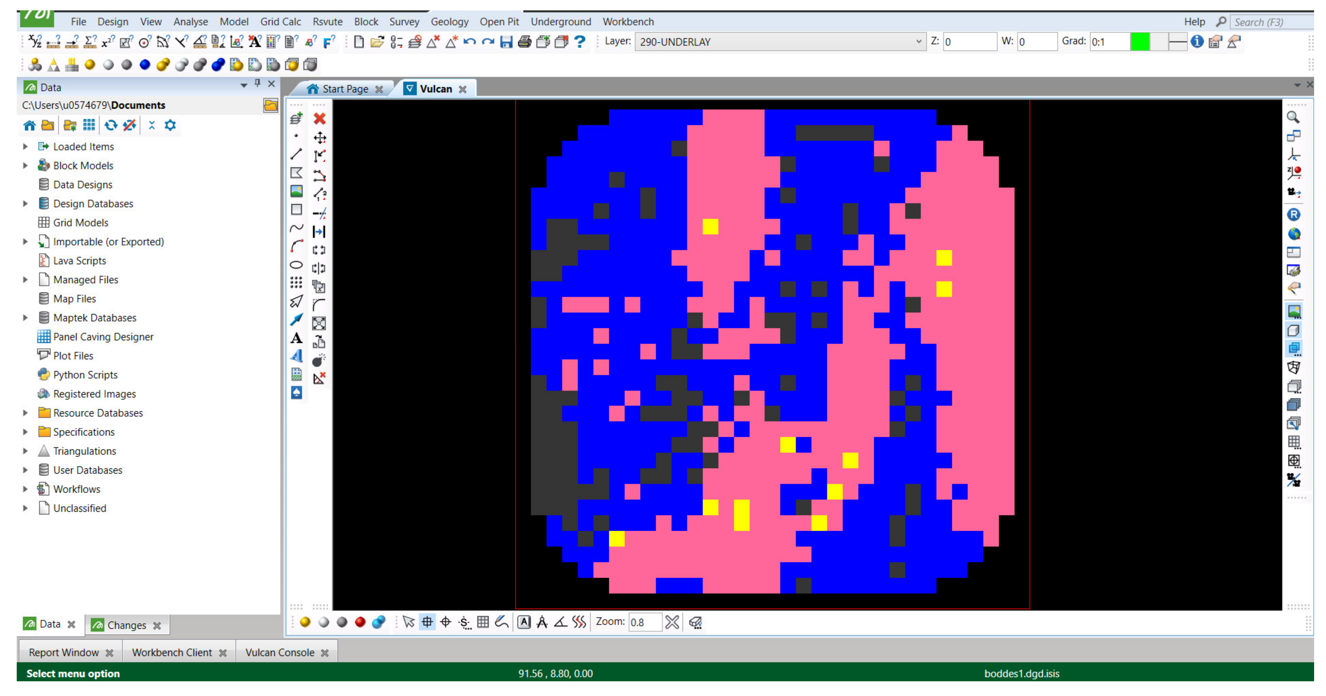
From the map shown in Figure 14, a block model may be created, since each coordinate is located on the same elevation, the block centroid Z-value is given by the elevation level midway through the bench. The block model shown in Figure 15 is the resulting block model from the interpolation shown in Figure 15 in Maptek Vulcan and bounded by the dimensions of the stockpile shown in Figure 7. To be clear, this block model contains only one block level. In the event that a stockpile contains multiple benches or levels, this same modelling process may be repeated for each level. Because the model was an interpolation, it populated values for every position within the sample space, including the corners where no data were shown. This interpolation is trimmed by the survey volume to create the block model shown in Figure 15.
Figure 15 shows grade values for each 5 m × 5 m × 5 m block in the example stockpile volume. Grade values are colored in accordance with the legend shown in the top left of the black viewing window of the screenshot. The red box represents the model extent area.
3.5. Analysis
To showcase the variance of the model by region and see how it compares with the data, confidence intervals on the mean values were used on each quadrant of the model area. A summary of the confidence intervals is shown in Table 3. Confidence intervals measure the degree of uncertainty in a dataset. They can take any number of probability limits, but Table 3 shows only 90%, 95% and 99% confidence levels. The greater the confidence interval value, the farther the mean value is from the remainder of the data.
Table 3 shows that for each quadrant and confidence level, the model has a smaller confidence interval value than that of the example data. Confidence interval values for the entire data area are only lower than two of the confidence intervals for the IDW model. These areas are in the bottom left and bottom right areas of the model and only when compared between a 90% confidence level with the data to a 99% confidence level with the model. Overall, these lower values demonstrate that the model has less variance than the dataset. The top half of the model also has less variance than the bottom half.
4. Discussion
4.1. Workflow
The controversy in using a method which incorporates FMS data is that it frequently disagrees with the reconciled grade values which are required for financial reporting. FMS data also contain errors and need to be cleaned before modelling can occur smoothly. However, FMS data can be integrated into an automatic modelling process which frees up engineering resources. Using a data-driven approach also acts as a step towards digitization, which will improve after each iteration.
Figure 15 demonstrates that this modelling method may be passed into conventional engineering software and used by mine operations to optimize the processing of the stockpile. Effectively, this makes stockpile processing similar to mining of a large muck pile and subject to the same methods of ore control and mine planning previously established. Engineering software can create an optimized sequence for processing the stockpile which reduces the variability of the feed entering the mill. Block information can be uploaded into modern shovels with tracking technology so that operators can more tightly control processing along expected grade boundaries.
Having knowledge of zones within the stockpile that are trending to higher or lower values could potentially lead the operation to plan the dumping locations of each blast pattern more thoroughly. The added cost of organizing the stockpile in a real-time optimization would need to be weighed against the expected savings in rehandle cost at the time of the processing of the stockpile years in the future. This cost analysis would be tricky to perform since there are many variables to consider and most mines do not know the exact values and tonnages of their low-grade ore to be mined over the course of the entire mine life.
4.2. Data
Some dump coordinates exist outside of survey areas. This may be due to errors in the FMS tracking capability, or some material may be initially dumped outside of the boundary and later moved into it via dozers or other heavy equipment. Since FMS data alone makes it hard to determine the extents of the topography, survey data will always need to be used to create a final trim. There are also issues in variability in the physical location of the GPS coordinate of the haul truck and how that exact position best relates to the centroid of the corresponding dump location. This difference makes an even greater impact in the upper layer or edge dumping case, where the area of influence of the truck is more one-dimensional.
Future data inputs from real-time surveying of stockpiles via UAVs can improve the z values substantially. Drone data can also be used to model the dumping by truck and the movement of material by dozers. Furthermore, drones and additional sensors, along with improved modeling of the spreading behavior can improve the basic assumptions of the model, thus improving understanding the relationships between the data and the model.
Despite including drone data, the ability to track material flow over the entirety of its life in a heap fill stockpile and through processing will likely remain out of reach. However, a generalized model of key components of truck-dumped stockpile material behavior (material flow during dumping and movement by dozers for example) will improve the ability to estimate characteristic distribution within stockpiles. This modelling could further reduce processing downtime and increase throughput during the eventual processing of the stockpile.
4.3. Modelling
Sampling can be used to verify or calibrate the model. If each truck is sampled individually, the average sampling density for the stockpile modelled would be equal to the haulage capacity of the truck used (100–400 t), which is an improvement in sampling density orders of magnitude above conventional sampling campaigns for heaped filled stockpiles and leach pads (175,000 tons in the use case of Winterton) [52]. While modelling will never replace sampling, both problems can be worked interdependently.
In the event that the grade and tonnage values differ substantially from official values given for financial reporting, the block model may be adjusted to represent the grade distribution of the stockpile as weighted by each block in comparison to all others and not strictly on block values given by interpolation of the FMS data. This adjustment to the model could also be completed in an autonomous manner and would involve data which are readily available at the mine.
The demonstration of FMS data incorporated into a stockpile block model in this paper opens the door to additional discussion around optimal stockpile modelling from FMS data. While the characteristic distribution of the material may not follow the inverse distance weighting method presented in this paper, it may be adequately modelled via other geostatistical methods, such as triangulation or nearest neighbors. Variograms, ordinary least squares (OLS) prediction methods, as well as kriging may also prove useful for stockpile modelling. These methods follow the modelling flowchart created by Pebesma [49] and shown as Figure 8.
Further studies and sampling could fine tune the model, such as using discrete element modeling for tracking flow of material for various settling scenarios. Once a model is deemed precise, which accurately accounts for the stockpile characteristics “as is”, more advanced models may account for metal degradation over time, natural leaching, and other environmental factors. These models may apply directly to heap leach operations by indicating target areas for hydrological work that could increase leaching capacity.
4.4. Other Factors
While the stockpile used in this study acts as a strategic form of storage, many of the stockpiles used in mining act as a buffer to ensure continuity of the processing stage. Stockpiles dedicated to maintaining a steady flow of material into the plant are generally beneficial. However, bottlenecks and data loss may affect the intention of keeping control of the flow of material from mine to plant. The short timeframe between stockpiling and processing these types of stockpiles means a different approach for modelling them should be used when compared with long-term stockpiles.
Exposure of stockpiles to dilution, weathering and other elements causes significant changes to their characteristics. These changes amount to degradation, which is more prevalent in long-term stockpiles. Rezakhah and Newman [42] quantify degradation to be between 5 and 10% annually and recognize that literature on the problem of degradation is often seen as isolated from stockpiling or mine planning problems. More robust models of stockpiles from historical FMS data could provide a more granular look into the distribution and rate of degradation which occurs within stockpiles over time.
Base and precious metal stockpiles have much in common, especially if they are made using haul trucks and dozers of the same size. Where base and precious metal stockpiles differ is due to geochemical characteristics of the ore as well as grade distribution differences (nugget effect). Base metals also oxidize quickly, which can affect the geotechnical stability of their stockpiles. These differences should be considered when developing a modelling approach for each of these types of stockpiled materials.
The model demonstrated in this paper takes a simplistic approach to the material in each truck load. In reality each truck load will likely have undergone some degree of pre-crusher blending. Shovels and loaders constantly mix the material and blast movement and dilution cause it to not reflect what is in the FMS data. Stockpiles that act as process buffers may also undergo additional blending both before and after crushing. In either type of stockpile, the effects of blending must be considered when modelling.
5. Conclusions
In conclusion, the type of working method demonstrated in this paper shows how leveraging FMS data and existing interpolation techniques can lead to increased understanding of the grade distribution within stockpiles. Figure 14 and Figure 15 indicate interpolated grade values at each location within the stockpile in a way which is directly incorporable into mining operations. Knowledge of the types of zones illustrated by Figure 14 and Figure 15 could enable miners to optimize the processing of their stockpiles. While this method is merely illustrative, it shows that through a systematic process of validation and modelling improvements, a given mine can use this method to come to a better understanding of the grade distribution within its long-term, low-grade stockpile. The implications of better modelling ROM stockpiles will enhance the overall mine optimization such as mine-to-mill and other continuous improvement initiatives at mines.
Author Contributions
Conceptualization, A.Y.; Data curation, A.Y.; Formal analysis, A.Y.; Funding acquisition, W.P.R.; Investigation, A.Y.; Methodology, A.Y.; Project administration, W.P.R.; Resources, W.P.R.; Software, A.Y.; Supervision, W.P.R. All authors have read and agreed to the published version of the manuscript.
Funding
This research received no external funding.
Data Availability Statement
The dataset used was made by the authors and is available upon request.
Acknowledgments
The authors would like to thank Newmont Mining Corporation for the collaboration and support of this project.
Conflicts of Interest
The authors declare no conflict of interest.
References
- Hustrulid, W.A. Open Pit Mine Planning & Design, 3rd ed.; Kuchta, M., Martin, R.K., Eds.; CRC Press: Boca Raton, FL, USA; Taylor & Francis Distributor: London, UK, 2013. [Google Scholar]
- Rogers, W.P.; Kahraman, M.M.; Dessureault, S. Exploring the value of using data: A case study of continuous improve-ment through data warehousing. Int. J. Min. Reclam. Environ. 2019, 33, 286–296. [Google Scholar] [CrossRef]
- Young, A.; Rogers, P. A Review of Digital Transformation in Mining. Min. Met. Explor. 2019, 36, 683–699. [Google Scholar] [CrossRef]
- Kanefsky, J.; Robey, J. Steam Engines in 18th-Century Britain: A Quantitative Assessment. Technol. Cult. 1980, 21, 161. [Google Scholar] [CrossRef]
- Mudd, G.M. Gold mining in Australia: Linking historical trends and environmental and resource sustainability. Environ. Sci. Policy 2007, 10, 629–644. [Google Scholar] [CrossRef]
- Zhang, K.; Kleit, A.N. Mining rate optimization considering the stockpiling: A theoretical economics and real option model. Resour. Policy 2016, 47, 87–94. [Google Scholar] [CrossRef]
- Optimum Determination of Sub-Grade Stockpiles in Open Pit Mines; The Australasian Institute of Mining and Metallurgy: Carlton, Australia, 1988.
- Brennan, M.J.; Schwartz, E.S. Evaluating Natural Resource Investments. J. Bus. 1985, 58, 135. [Google Scholar] [CrossRef] [Green Version]
- Lane, K.F. The Economic Definition of Ore: Cut-Off Grades in Theory and Practice; Mining Journal Books: London, UK, 1988. [Google Scholar]
- Menabde, M. Mining Schedule Optimisation for Conditionally Simulated Orebodies. In Advances in Applied Strategic Mine Planning; Dimitrakopoulos, R., Ed.; Springer International Publishing: Cham, Switzerland, 2018; pp. 91–100. [Google Scholar]
- Asad, M.W.A. Cutoff grade optimization algorithm with stockpiling option for open pit mining operations of two economic minerals. Int. J. Surf. Min. Reclam. Environ. 2005, 19, 176–187. [Google Scholar] [CrossRef]
- Asad, M.W.A.; Dimitrakopoulos, R. Optimal production scale of open pit mining operations with uncertain metal supply and long-term stockpiles. Resour. Policy 2012, 37, 81–89. [Google Scholar] [CrossRef]
- Chanda, E.; Dagdelen, K. Optimal blending of mine production using goal programming and interactive graphics systems. Int. J. Surf. Min. Reclam. Environ. 1995, 9, 203–208. [Google Scholar] [CrossRef]
- Gu, Q.; Lu, C.; Guo, J.; Jing, S. Dynamic management system of ore blending in an open pit mine based on GIS/GPS/GPRS. Min. Sci. Technol. (China) 2010, 20, 132–137. [Google Scholar] [CrossRef]
- Jupp, K.; Howard, T.J.; Everett, J.E. Role of pre-crusher stockpiling for grade control in iron ore mining. Appl. Earth Sci. 2013, 122, 242–255. [Google Scholar] [CrossRef]
- Everett, J. Simulation Modeling of an Iron Ore Operation to Enable Informed Planning. Interdiscip. J. Inf. Knowl. Manag. 2010, 5, 101–114. [Google Scholar] [CrossRef] [Green Version]
- Everett, J.E.; Howard, T.J.; Jupp, K. Simulation modelling of grade variability for iron ore mining, crushing, stockpiling and ship loading operations. Min. Technol. 2010, 119, 22–30. [Google Scholar] [CrossRef]
- Carter, R.A. Staying on Top of Stockpile Management. Eng. Min. J. 2018, 219, 58. [Google Scholar]
- Vangold Resources Completes Acquisition of Historic El Pinguico Mine, Guanajuato, Mexico. Accesswire, Junior Mining Network. 2017. Available online: https://www.juniorminingnetwork.com/junior-miner-news/press-releases/1961-tsx-venture/gsvr/31757-vangold-resourcescompletes-acquisition-of-historic-el-pinguico-mine-guanajuato-mexico.html (accessed on 10 June 2021).
- Preece, H. Gencor is Building up Stockpile of Gold Ore, in American Metal Market. 1986. Gale General OneFile. Available online: www.gale.com/apps/doc/A4256121/ITOF?u=marriottlibrary&sid=bookmark-ITOF&xid=edcc5334 (accessed on 10 June 2021).
- Bulbeck, C. The Iron Ore Stockpile and Dispute Activity in the Pilbara. J. Ind. Relat. 1983, 25, 431–444. [Google Scholar] [CrossRef]
- Ozols, V. Anvil Range to Shutter Mine: Company Will Process Ore from Existing Stockpile, in American Metal Market. 1996. Gale General OneFile. Available online: www.gale.com/apps/doc/A18883408/ITOF?u=marriottlibrary&sid=bookmark-ITOF&xid=c27bb2d5 (accessed on 10 June 2021).
- Koushavand, B.; Askari-Nasab, H.; Deutsch, C.V. A linear programming model for long-term mine planning in the presence of grade uncertainty and a stockpile. Int. J. Min. Sci. Technol. 2014, 24, 451–459. [Google Scholar] [CrossRef]
- Zhao, S.; Lu, T.-F.; Koch, B.; Hurdsman, A. 3D stockpile modelling and quality calculation for continuous stockpile management. Int. J. Min. Process. 2015, 140, 32–42. [Google Scholar] [CrossRef]
- Zhao, S.; Lu, T.-F.; Koch, B.; Hurdsman, A. Stockpile Modelling Using Mobile Laser Scanner for Quality Grade Control in Stockpile Management. In Proceedings of the 2012 12th International Conference on Control Automation Robotics & Vision (ICARCV), Guangzhou, China, 5–7 December 2012; pp. 811–816. [Google Scholar]
- Sensogut, C.; Ozdeniz, A.H. Statistical modelling of stockpile behaviour under different atmospheric condi-tions—Western Lignite Corporation (WLC) case. Fuel 2005, 84, 1858–1863. [Google Scholar] [CrossRef]
- Kasmaee, S. Reserve estimation of the high phosphorous stockpile at the Choghart iron mine of Iran using geostatisti-cal modeling. Min. Sci. Technol. (China) 2010, 20, 855–860. [Google Scholar] [CrossRef]
- Morley, C.; Arvidson, H. Mine value chain reconciliation-demonstrating value through best practice. In Proceedings of the Tenth International Mining Geology Conference, Hobart, Tasmania, 20–22 September 2017; pp. 20–22. [Google Scholar]
- Hawley, M.; Cunning, J. Guidelines for Mine Waste Dump and Stockpile Design; CSIRO Publishing: Clayton, Australia, 2017. [Google Scholar]
- Parker, B.M. The Simulation and Analysis of Particle Flow Through an Aggregate Stockpile. Ph.D. Thesis, Virginia Tech, Blacksburg, VA, USA, 2009. [Google Scholar]
- Afrapoli, A.M.; Askari-Nasab, H. Mining fleet management systems: A review of models and algorithms. Int. J. Min. Reclam. Environ. 2017, 33, 42–60. [Google Scholar] [CrossRef]
- Jansen, W. Tracer-based mine-mill ore tracking via process hold-ups at Northparkes mine. In Proceedings of the Tenth Mill Operators’ Conference, Adelaide, Australia, 12 October 2009; pp. 12–14. [Google Scholar]
- Jurdziak, L.; Kawalec, W.; Król, R. Study on Tracking the Mined Ore Compound with the Use of Process Analytic Tech-nology Tags. In Intelligent Systems in Production Engineering and Maintenance—ISPEM 2017; Springer International Publishing: Cham, Switzerland, 2018. [Google Scholar]
- Ge, L.; Li, X.; Ng, A.H.-M. UAV for mining applications: A case study at an open-cut mine and a longwall mine in New South Wales, Australia. In Proceedings of the 2016 IEEE International Geoscience and Remote Sensing Symposium (IGARSS), Beijing, China, 10–15 July 2016; pp. 5422–5425. [Google Scholar] [CrossRef]
- Rathore, I.; Kumar, N.P. Unlocking the potentiality of uavs in mining industry and its implications. International Journal of Innovative Research in Science. Eng. Technol. 2015, 4, 852–855. [Google Scholar]
- Goldratt, E.M.; Cox, J. The Goal: A Process of Ongoing Improvement; North River Press: Great Barrington, MA, USA, 2012. [Google Scholar]
- Kahraman, M.M.; Rogers, W.P.; Dessureault, S. Bottleneck identification and ranking model for mine operations. Prod. Plan. Control 2020, 31, 1178–1194. [Google Scholar] [CrossRef]
- Sarle, W.S. Prediction with missing inputs. Jcis 98 Proc. 1998, 2, 399–402. [Google Scholar]
- Sarbanes, P. Sarbanes-Oxley act of 2002. In The Public Company Accounting Reform and Investor Protection Act; US Congress: Washington, DC, USA, 20 July 2002. [Google Scholar]
- Macfarlane, A. Reconciliation along the mining value chain. J. S. Afr. Inst. Min. Met. 2015, 115, 679–685. [Google Scholar] [CrossRef]
- Ghorbani, Y.; Nwaila, G.T.; Chirisa, M. Systematic Framework toward a Highly Reliable Approach in Metal Accounting. Min. Process. Extr. Met. Rev. 2020, 1–15. [Google Scholar] [CrossRef]
- Rezakhah, M.; Newman, A. Open pit mine planning with degradation due to stockpiling. Comput. Oper. Res. 2020, 115, 104589. [Google Scholar] [CrossRef]
- Engström, K. A comprehensive literature review reflecting fifteen years of debate regarding the representativity of reverse circulation vs blast hole drill sampling. TOS Forum 2013, 2013, 36. [Google Scholar] [CrossRef]
- Thornton, D. The implications of blast-induced movement to grade control. In Proceedings of the Seventh International Mining Geology Conference, Perth, Australia, 17 August 2009; pp. 287–300. [Google Scholar]
- Abzalov, M.Z.; Menzel, B.; Wlasenko, M.; Phillips, J. Optimisation of the grade control procedures at the Yandi iron-ore mine, Western Australia: Geostatistical approach. Appl. Earth Sci. 2010, 119, 132–142. [Google Scholar] [CrossRef]
- Ortiz, M.J.; Magri, E.J. Designing an advanced RC drilling grid for short-term planning in open pit mines: Three case studies. J. S. Afr. Inst. Min. Met. 2014, 114, 631–639. [Google Scholar]
- Subramaniyan, M.; Skoogh, A.; Muhammad, A.S.; Bokrantz, J.; Johansson, B.; Roser, C. A data-driven approach to diagnosing throughput bottlenecks from a maintenance perspective. Comput. Ind. Eng. 2020, 150, 106851. [Google Scholar] [CrossRef]
- Pyrcz, M.J.; Deutsch, C.V. Geostatistical Reservoir Modeling; Oxford University Press: Hong Kong, China, 2014. [Google Scholar]
- Pebesma, E.; Wesseling, C.G. Gstat: A program for geostatistical modelling, prediction and simulation. Comput. Geosci. 1998, 24, 17–31. [Google Scholar] [CrossRef]
- Burrough, P. Principles of geographical information systems for land resources assessment. Geocarto Int. 1986, 1, 54. [Google Scholar] [CrossRef]
- Bartier, P.M.; Keller, C. Multivariate interpolation to incorporate thematic surface data using inverse distance weighting (IDW). Comput. Geosci. 1996, 22, 795–799. [Google Scholar] [CrossRef]
- Winterton, J. Estimating the Residual Inventory of A Large Gold Heap Leach Pad; Society for Mining, Metallurgy & Exploration: Englewood, CO, USA, 2013. [Google Scholar]

Figure 2.
Types of Stockpile Fill (adapted from [29]).
Figure 2.
Types of Stockpile Fill (adapted from [29]).

Figure 3.
Digital Gaps in Different Phases of Mining Operation.

Figure 4.
Reserve and Operational Models.

Figure 5.
Research Approach Following a Data-Driven [47] Technique.
Figure 5.
Research Approach Following a Data-Driven [47] Technique.

Figure 6.
Data Flow Overview Figure.

Figure 7.
Screenshot of Hypothetical Heaped Fill Stockpile Designed in Maptek Vulcan.
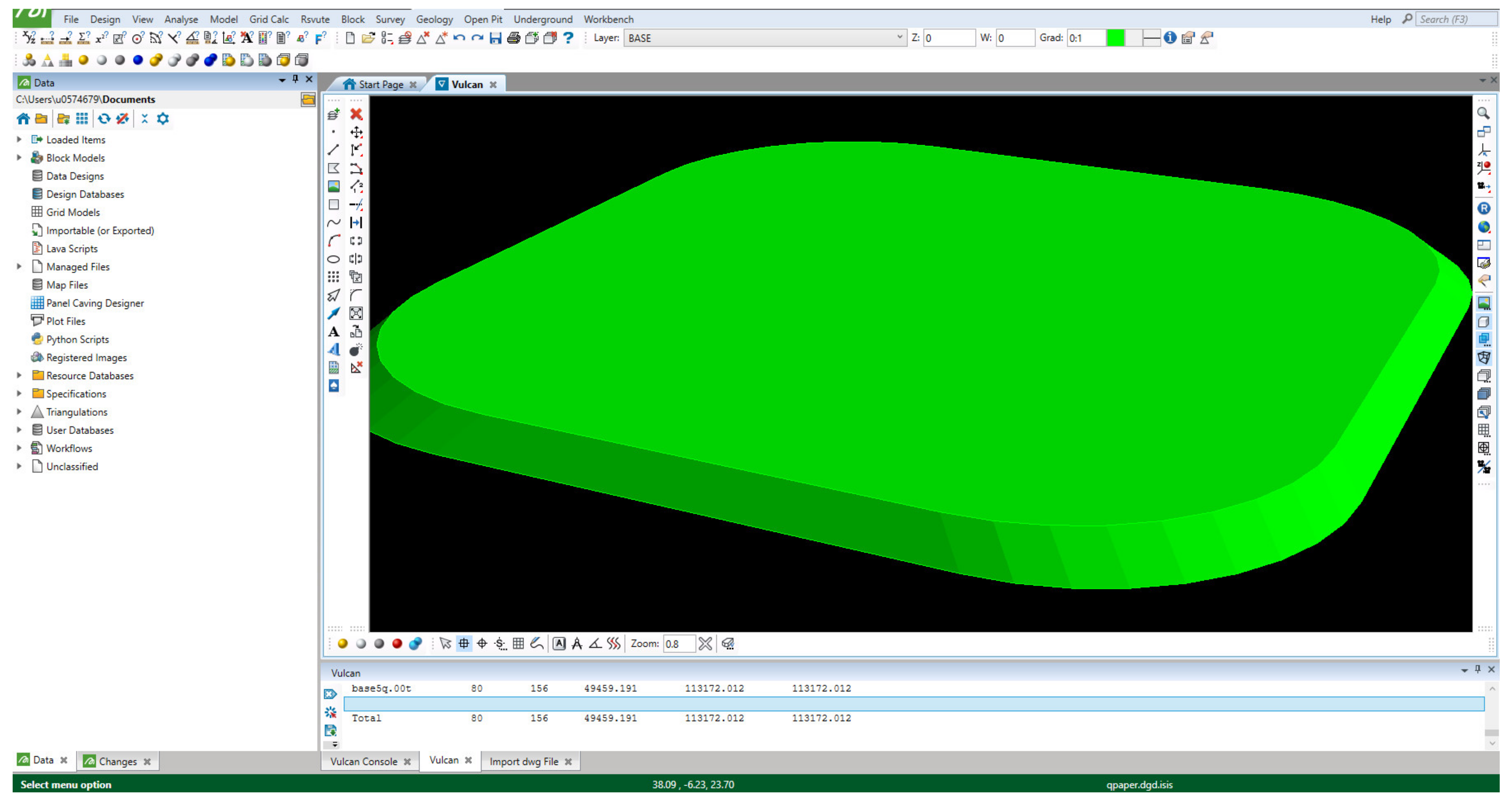
Figure 8.
Decision Tree for Default gstats Program Action (from Pebesma [49]).
Figure 8.
Decision Tree for Default gstats Program Action (from Pebesma [49]).

Figure 9.
Visualization of FMS Data.

Figure 10.
Base Layer Grade Dumps of Example Stockpile Colored by Grade.

Figure 11.
Volume of Influence of Haul Truck in Paddock Dumping Case.

Figure 12.
Upper Layer Dumps of an Example Stockpile Colored by Grade.

Figure 13.
Assumed Area of Influence of Haul Truck in Edge Dumping Scenarios.

Figure 14.
Grade Distribution Map of Combination of Layers.

Figure 15.
Screenshot in Maptek Vulcan of Resulting Block Model from FMS Data Interpolation.

Table 1.
Example FMS and Assay Data Categories.
| Timestamp | Grade ID | Au g/t | Actual Dumping Location | Dump Coordinate Easting | Dump Coordinate Northing | Dump Tonnage |
|---|---|---|---|---|---|---|
| Date and Time of Dump | Unique Grade Pattern of Material Dumped | Au Grade value in g/t | Name and bench height of dump location polygon | Easting coordinate of dump location | Northing coordinate of dump location | Tonnage of material dumped |
Table 2.
Statistical Characteristics of the Modelling Dataset.
| Spatial Data | |||||||
|---|---|---|---|---|---|---|---|
| Number of Points | 963 | ||||||
| X min (m) | X Max (m) | Y Min (m) | Y Max (m) | ||||
| 5 | 145 | 5 | 150 | ||||
| Grade Data | |||||||
| Grade Unit | Grams per ton (g/t) | ||||||
| Minimum | 1st Quartile | Mean | Median | 3rd Quartile | Maximum | ||
| 0.3 | 0.33 | 0.3952 | 0.37 | 0.47 | 0.57 | ||
Table 3.
Confidence Intervals of Data and Model Areas.
| Example Data | All Area | Bottom Left | Bottom Right | Top Left | Top Right |
|---|---|---|---|---|---|
| Confidence Level (90.0%) | 0.004606 | 0.005712376 | 0.005165079 | 0.005724806 | 0.005109 |
| Confidence Level (95.0%) | 0.00549 | 0.006809497 | 0.006156908 | 0.006824275 | 0.006090 |
| Confidence Level (99.0%) | 0.007221 | 0.008958197 | 0.008099109 | 0.008977509 | 0.008011 |
| IDW Model | All Area | Bottom Left | Bottom Right | Top Left | Top Right |
| Confidence Level (90.0%) | 0.001927 | 0.003029155 | 0.003031626 | 0.002473611 | 0.002453 |
| Confidence Level (95.0%) | 0.002297 | 0.003611474 | 0.003614413 | 0.002948945 | 0.002924 |
| Confidence Level (99.0%) | 0.003021 | 0.004752802 | 0.004756644 | 0.003880283 | 0.003847 |
Publisher’s Note: MDPI stays neutral with regard to jurisdictional claims in published maps and institutional affiliations. |
© 2021 by the authors. Licensee MDPI, Basel, Switzerland. This article is an open access article distributed under the terms and conditions of the Creative Commons Attribution (CC BY) license (https://creativecommons.org/licenses/by/4.0/).
Share and Cite
MDPI and ACS Style
Young, A.; Rogers, W.P. Modelling Large Heaped Fill Stockpiles Using FMS Data. Minerals 2021, 11, 636. https://doi.org/10.3390/min11060636
AMA Style
Young A, Rogers WP. Modelling Large Heaped Fill Stockpiles Using FMS Data. Minerals. 2021; 11(6):636. https://doi.org/10.3390/min11060636
Chicago/Turabian StyleYoung, Aaron, and William Pratt Rogers. 2021. "Modelling Large Heaped Fill Stockpiles Using FMS Data" Minerals 11, no. 6: 636. https://doi.org/10.3390/min11060636
Note that from the first issue of 2016, this journal uses article numbers instead of page numbers. See further details here.