The (U-Th)/He Chronology and Geochemistry of Ferruginous Nodules and Pisoliths Formed in the Paleochannel Environments at the Garden Well Gold Deposit, Yilgarn Craton of Western Australia: Implications for Landscape Evolution and Geochemical Exploration

Abstract

Ferruginous nodules and pisoliths that cap deeply weathered profiles and transported cover are characteristic of the Yilgarn Craton, Western Australia. Here we show how ferruginous nodules and pisoliths formed in the paleochannel sediments during Miocene can be used to locate buried Au mineralization. Three types of ferruginous nodules and pisoliths were identified in paleochannel sediments and saprolite, representing different parent materials and environments covering the Garden Well Au deposit: (i) ferruginous nodules formed in saprolite on the flanks of the paleochannel (NSP), (ii) ferruginous pisoliths formed in the Perkolilli Shale in the middle of the paleochannel (PPS) and (iii) ferruginous nodules formed in the Wollubar Sandstone at the bottom of the paleochannel (NWS). The appearance, mineralogy and geochemistry of ferruginous nodules and pisoliths vary according to their origin. The PPS and NWS are goethite-rich whereas NSP is a mixture of goethite and hematite which make them all suitable for (U–Th)/He dating. The average age of goethite in the NSP is 14.8 Ma, in the NWS is 11.2 Ma and in the PPS is 18.6 and 14 Ma. The goethite ages in ferruginous nodules and pisoliths are thought to be younger than the underlying saprolite (Paleocene-Eocene) and were formed in different environmental conditions than the underlying saprolite. Anomalous concentrations of Au, As, Cu, Sb, In, Se, Bi, and S in the cores and cortices of the NWS and the PPS reflect the underlying Au mineralization, and thus these nodules and pisoliths are useful sample media for geochemical exploration in this area. These elements originating in mineralized saprolite have migrated both upwards and laterally into the NWS and the PPS, to form spatially large targets for mineral exploration.

1. Introduction

In Australia, exploration is progressively moving to areas of deep transported cover (>20 m) as more easy areas become exhausted. Given the cost of deep drilling, high-density sampling of the weathered basement beneath the unconformity is no longer cost-effective. Conventional approaches (e.g., soil and lag sampling) may not be applicable in areas of transported cover, and various selective extraction methods and gases have had only limited success, so there is a need for new approaches. A variety of transported cover sediments, ranging from Quaternary to Permian, are common in the Yilgarn Craton of Western Australia [1]. These have been subjected to weathering, especially the Tertiary paleochannel sediments. Sampling these sediments presents challenges because of their exotic origin and variably weathered character, but their weathering products also present opportunities, as they may contain mechanical and/or hydromorphic characteristics from concealed mineralization. The most common post-depositional weathering product of the paleochannel sediments is ferruginous nodules and pisoliths. A first step towards grasping the complexities of the ferruginous nodules and pisoliths is to understand the effects that geochronology and past climates have had on their development and geochemistry.

Dating of weathering profiles and sediments provides useful information on paleoclimates and rates of landscape evolution. In mineralized areas, it may also provide insight into the timing and rates of dissolution of indicator elements, and their transport and reprecipitation. Of the variety of ferruginous materials in the regolith of the Yilgarn Craton [1], mainly two types have been dated using paleomagnetism and (U–Th)/He methods. These are hematite-rich mottles in saprolite and hematite-goethite-maghemite-rich ferruginous nodules and pisoliths [2,3]. Paleomagnetic dating of hematitic mottles in saprolite from several locations in the arid eastern Yilgarn Craton yields Paleocene to Eocene and Miocene ages with some evidence of earlier weathering [4]. This provides the minimum age of saprolite formation but there are no dating studies of the corresponding widespread ferruginous nodules and pisoliths overlying saprolite on the arid eastern Yilgarn Craton. However, two studies were conducted in the western Yilgarn Craton which has a Mediterranean climate. An initial study by [2] and later by [3] demonstrated that (U–Th)/He dating could be used on hematite-goethite-maghemite-rich ferruginous nodules and pisoliths developed in a deeply weathered bauxitic profile in the western Yilgarn Craton. (U–Th)/He dating yielded dates of 1.3 to 10 Ma for ferruginous nodules and pisoliths. Since goethite and hematite formation is the main process generating the ferruginous nodules and pisoliths, dating authigenic Fe oxyhydroxide constrains minimum limits on their age of formation [3,5].

We have carried out dating and metal dispersion investigations for ferruginous nodules and pisoliths in the eastern Yilgarn using samples from the Garden Well Au deposit. The Garden Well Au deposit area is an example of regolith situations i and iii (see below Section 2) and is used here to document and better understand the characteristics, timing of formation, and geochemical and mineralogical signatures of the Au deposit in ferruginous nodules and pisoliths buried beneath paleochannels. Here, we also show that ferruginous nodules and pisoliths occurring at the unconformity and formed higher in paleochannel sediments can retain geochemical signatures resulting from hydromorphic and clastic dispersion of the underlying Au mineralization.

2. Ferruginous Nodules and Pisoliths in Context of Landscape of the Yilgarn Craton

The landscape of the Yilgarn Craton is a gently undulating surface surrounded by dissected hills. Paleochannels have long been recognized in the regolith of the Yilgarn Craton [1,6,7,8,9]. The landscape has experienced several episodes of erosion and deposition punctuated by periods of relative stability during which weathering profiles and their ferruginous materials formed. Thus, ferruginous nodules and pisoliths have formed in a variety of weathering and sedimentary environments [1]. They have not only formed from weathering of bedrock but are also common in transported cover.

Ferruginous pisoliths are spherical, and nodules are generally irregular, but smooth in shape [10]. Ferruginous pisoliths have a variety of nuclei surrounded by an outer skin or cortex. The cortex may be composed of a number of layers termed laminae similar to an onion. Ferruginous nodules may or may not have a cortex. Ferruginous nodules and pisoliths occur in three environments in the Yilgarn Craton [1]. These include:

I. Where there has been minimal or a lack of erosion of upland weathered bedrock has occurred, ferruginous nodules and pisoliths (NSP) are found typically downslope from subdued weathered bedrock hills and proximal to paleochannels with less than 15 m of deep transported cover (Figure 1). Here, a prominent breakaway scarp is not developed because saprolite on low hills is generally ferruginized or silicified which is resistance to erosion best exemplified on greenstone terrain.

II. Where upland weathered bedrock is attacked by erosion, resistant duricrust occupies topographically higher areas as prominent breakaway scarps (erosional escarpment) typical of granitic terrain (Figure 1). Deeply weathered granites and gneisses erode relatively easily because of weak ferruginization. Immediately below the breakaways, the low hills and pediments are dominated by a thinner mantle of saprolite, saprock, and fresh bedrock. Backslopes behind the breakaways continue to host ferruginous nodules and pisoliths formed in saprolite and local colluvium (NSP) under the varying thickness of transported cover [1].

III. Ferruginization of paleochannel sediments leads to ferruginous nodules and pisoliths that occur at the base of the paleochannel sequence (NWS) and are also commonly randomly distributed higher in the sequence (PPS; Figure 1).

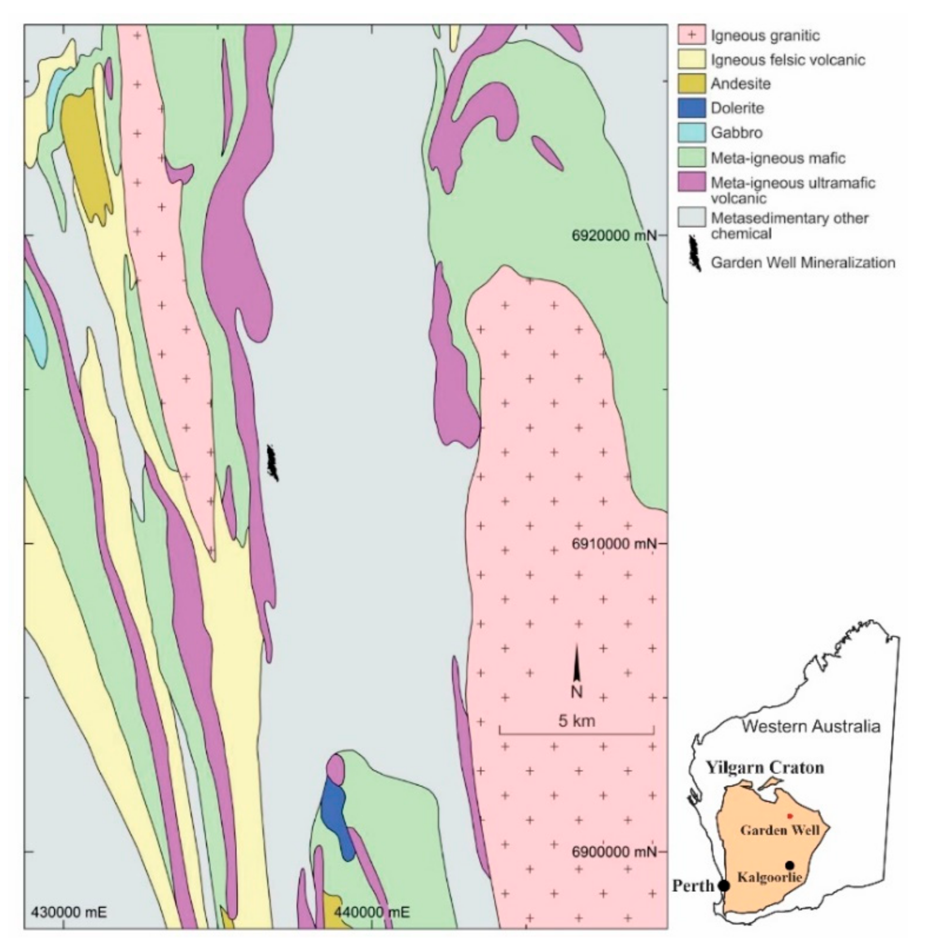
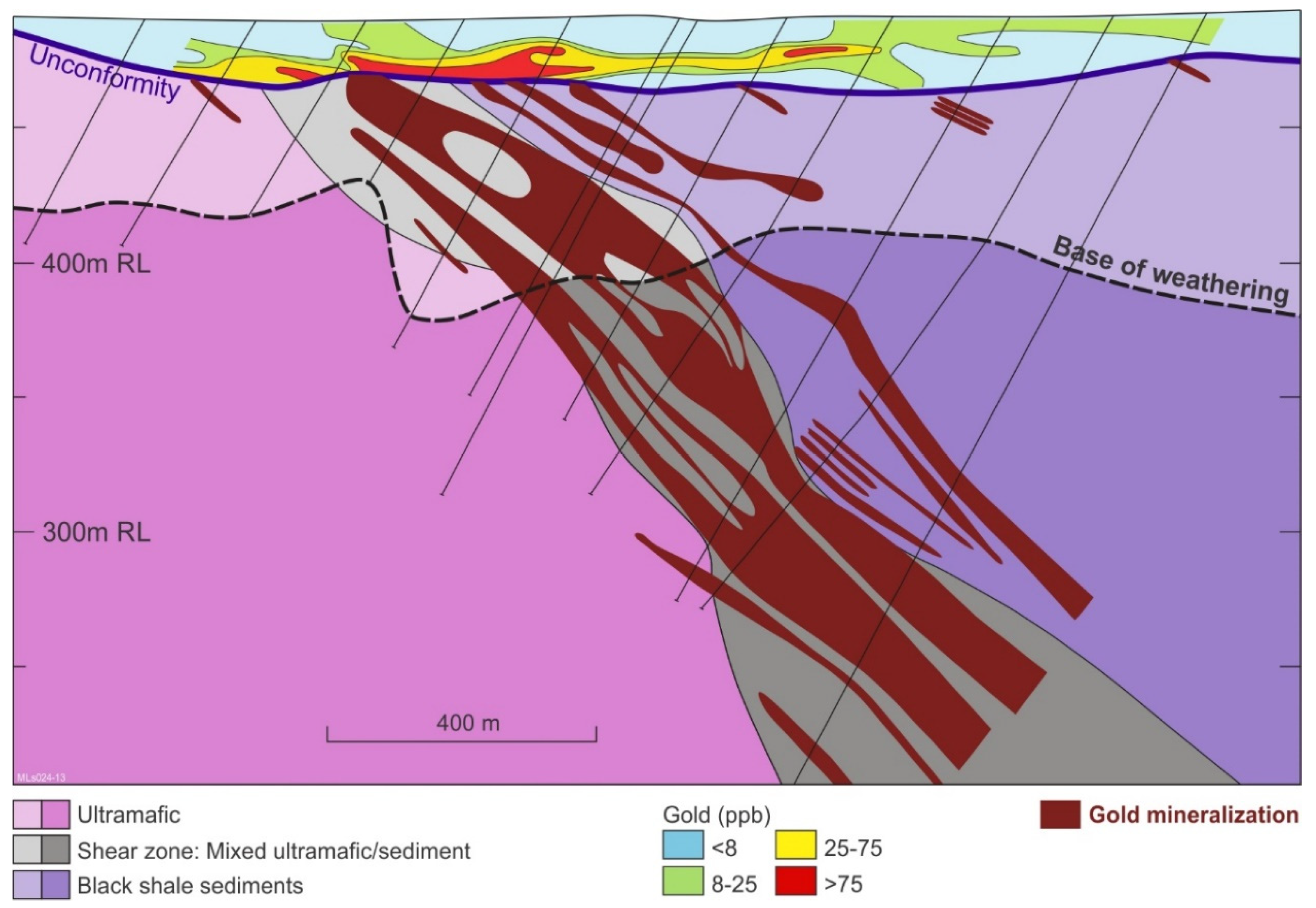
3. Geology and Mineralization

The Garden Well Au deposit is located approximately 1000 km north-northeast of Perth in Western Australia (Figure 2). It lies within the Duketon greenstone belt in the northern part of the Eastern Goldfields Province of the Archean Yilgarn Craton. The Eastern Goldfields Province is a typical Archaean granite–greenstone terrain, characterized by large areas of granitoid and gneiss adjacent to linear to arcuate, north-northwesterly trending greenstone belts. At its widest point, the Duketon greenstone belt is approximately 30 km across and comprises a deeply weathered sequence of deformed and metamorphosed ultramafic, mafic, and felsic volcanic rocks, with associated volcaniclastic sedimentary rocks (Figure 2; [11]). Thin units of banded chert and banded Fe formation also occur. Late-stage, high-level, felsic to intermediate sills, dykes, and small plutons intrude the sequence [11].

The Garden Well Au deposit is the largest and most recent Au discovery in the Duketon greenstone belt with an indicated resource of 2.47 Moz and a reserve of 1.1 Moz [13]. It is located on the eastern limb of the Erlistoun Syncline in a narrow, regional N-S trending structure defined by intense shearing and faulting [13]. Here deep weathering and a shallow paleochannel have developed, hindering exploration [13]. The Garden Well Au deposit is concealed by Eocene paleochannel sediments up to 35 m thick (Figure 3). There are no historical gold workings or previous drilling associated with the deposit, and there has been no response to conventional geochemical and geophysical exploration methods [13]. However, surficial Au concentrations on flanking rises adjacent to the deposit reach 8–75 ppb Au in ferruginous lag.

The Archean stratigraphy under the paleochannel consists of a 1.5 km thick N-S moderately east-dipping high to moderate MgO (20–35%) komatiite flows that form the footwall to the Au mineralization. The ultramafic rocks have undergone greenschist metamorphism to serpentine and carbonate and now have talc-dolomite-chlorite-tremolite-serpentine mineralogy [13]. The ultramafic sequence is overlain by 1400 m of black carbonaceous shales, cherts, and thin BIFs, which dip to the east. The shear zone hosting Au mineralization at Garden Well is located on the footwall of the sedimentary package overlain by the ultramafic unit. The shear zone is several hundred meters wide, dips 60° east, and is subparallel to the sedimentary contact. Intense shearing along the sedimentary contact is contained within a mixed ultramafic-sedimentary package that hosts the Au mineralization [13].

Gold mineralization (1–2 g/t Au) occurs as oxide ore down to 70 m below the base of the paleochannel, and the hypogene ore (1.0 g/t Au) extends to 400 m (Figure 3). Lead, Zn, and Cu sulfides occur within the ore. Oxide mineralization consists of a 70 to 100 m wide, moderately east-dipping Au-bearing zone in clay-rich saprolite with some sub-horizontal supergene Au developed in the upper part of the saprolite profile. Anomalous Au occurs in the bottom 15 m of the paleochannel. The shear zone continues as primary hypogene mineralization below the top of fresh rock and is characterized by a 50–70 m wide, strongly altered quartz–dolomite–fuchsite–chlorite–pyrite zone in ultramafic rocks.

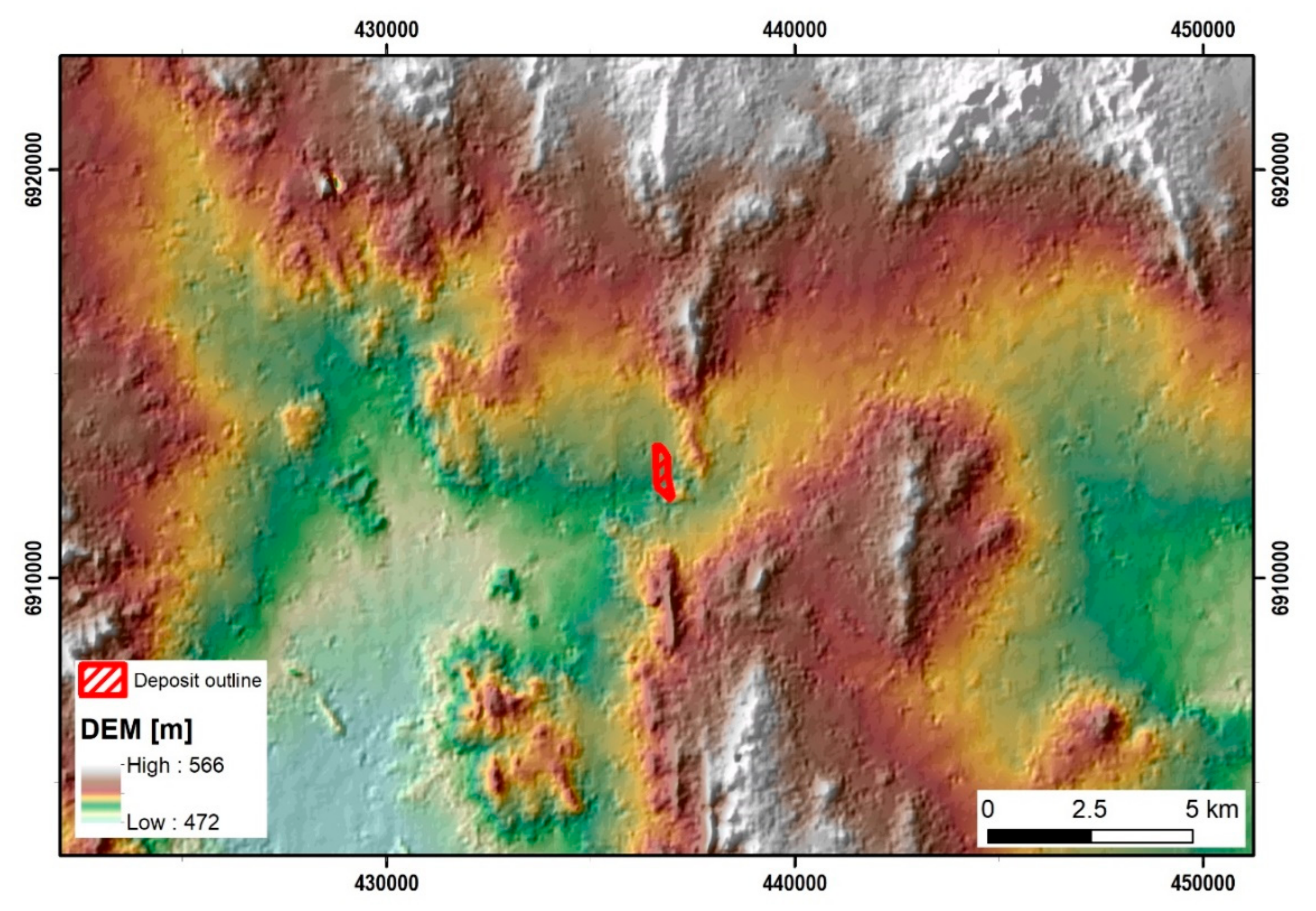
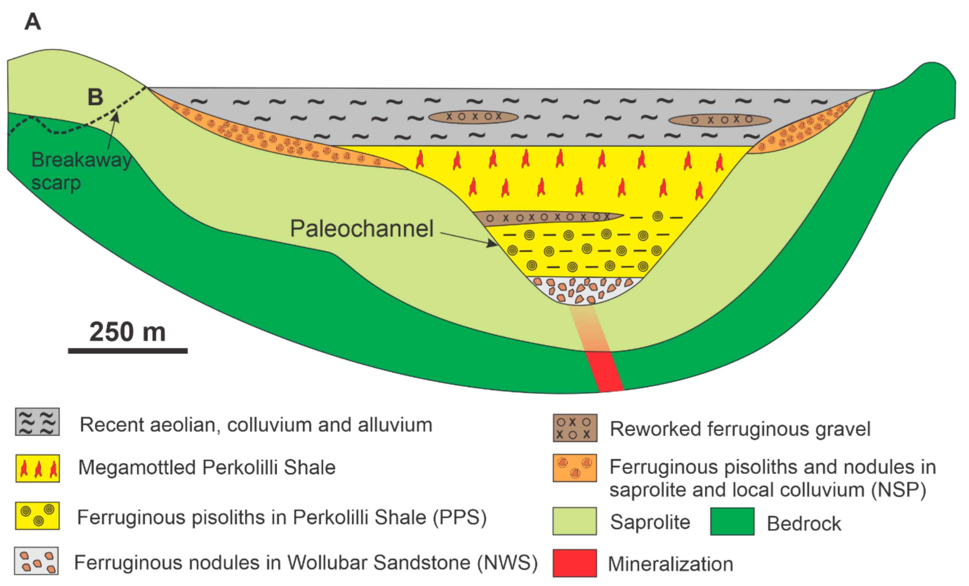
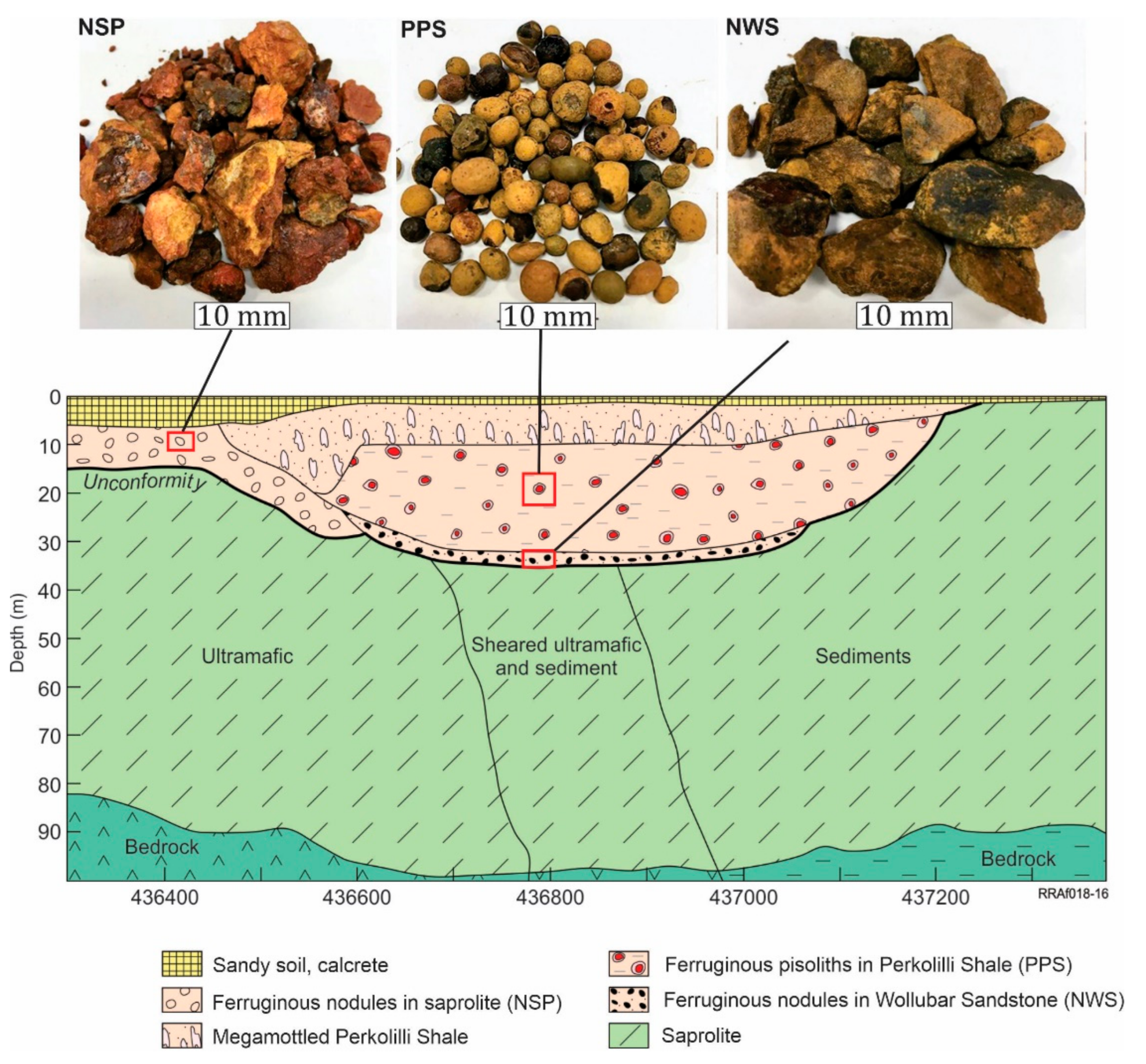
4. Geomorphology and Ferruginous Nodules and Pisoliths in the Garden Well Deposit and its Nearby Environments

The landforms in the Garden Well area were largely formed by erosion, dissection, and in-fill of a deeply weathered land surface. There are two distinct groups of landforms related to the underlying geology. Areas underlain by greenstone are characterized by subdued strike ridges and low, rounded hills of ferruginous saprolite and ferruginous debris. In contrast, areas underlain by granite are characterized by extensive sand sheets and scattered exposures of weathered rock with well-developed breakaways.

The Garden Well area is generally flat to undulating, ranging in altitude from an average of 560 m in the north to 480 m in the south. The main physiographic features are the broad valley of Borodale Creek, which trends southeast through the center of the area, with subdued topographic highs along each side of the valley. The Garden Well deposit lies in the ephemeral north-south drainage of Mistake Creek (Figure 4) in a paleo valley that runs into Borodale Creek and then into the Lake Carey saline lake system about 50 km to the southwest [14]. The physiography surrounding the Garden Well deposit (490 m) is of relatively low relief (70 m). The valley is surrounded by subdued saprock hills and a ridge of BIF in the eastern part of the area. Topographic lows hosting the ephemeral drainage system reach 470 m above mean sea level at a similar distance to the southwest. Standing bodies of water are rare, but there is one close to the deposit on Mistake Creek. Sandy areas rapidly absorb light rain but heavier falls result in sheet flooding run-off.

At the Garden Well deposit, within the valley, there is a paleochannel up to 35 m deep and ~600 m wide that runs north-south to the west of the saprock hill and dominates the central part of the study area (Figure 5). The paleochannel is steeply incised into saprolite, which is up to 80 m thick. The paleochannel is symmetric and U-shaped with a moderately broad valley floor with gently inclined straight side-slopes (Figure 5). The side slopes are mantled by 5–10 m of NSP. Ferruginous nodules overlie saprolite, which, in turn, are overlain by 2–5 m of recent colluvium and alluvium.

The stratigraphy of paleochannels at Garden Well is broadly similar to other locations where pisoliths have been developed [1,6,8,9,15]. At Garden Well, the paleochannel is composed of two Formations that are overlain by sandy soil and calcrete. The basal fluviatile formation, termed the Wollubar Sandstone [6], rests unconformably on the saprolite. It is unconformably overlain by the Perkolilli Shale [1,6]. In some parts of the section, dolomite cuts across lithological contacts, extending down into the Wollubar Sandstone and into the weathered basement. The Wollubar Sandstone (palynologically dated as Late Middle to Early Late Eocene) is composed of 1–4 m of fine to medium-grained sand cemented by Fe to form ferruginous nodules at the unconformity (NWS; Figure 5). A 20–30 m thick sequence of the Late Eocene Perkolilli Shale consists of red to grey kaolinitic clays with small amounts of smectite and fine-grained, sub-angular quartz grains. Most of the kaolinite within the clay unit is detrital and was probably derived from deeply weathered Archean basement rocks. The Perkolilli Shale has undergone post-depositional weathering, resulting in mobilization and redeposition of Fe as oxides and oxyhydroxides. By far the most conspicuous structures in the Perkolilli Shale are ferruginous pisoliths and mega mottles of Fe oxide accumulations. Ferruginous pisoliths are most abundant in the middle and base of the clay, where they form a conspicuous matrix- supported fabric. It is important to note that although the pisoliths are characteristic of the Perkolilli Shale, they occupy only 20–25% of the clay unit. Several workers [1,9,16,17]. have noted that ferruginous pisoliths are widespread and ubiquitous within the Perkolilli Shale and have been found in separate paleochannels over 300 km apart [1,9]. Above the pisolitic clays lie the hematitic mega mottled kaolinitic clays. Finally, the sequence is overlain by 1–2 m of calcareous to siliceous colluvium and alluvium and red-brown sandy soil and polymictic gravel. Drying of the climate led to the deposition of these sediments that buried and obscured the paleochannels.

Figure 4. DEM of the Garden Well area showing general physiography [18] and Regis Resources). The outline of the Garden Well deposit is shown.

Figure 4. DEM of the Garden Well area showing general physiography [18] and Regis Resources). The outline of the Garden Well deposit is shown.

The groundwater at Garden Well is very shallow (2–5 m depth) and is anomalous in Au (up to 610 ppt) and As (up to 7.9 ppb) [14]. Other elements of importance are Ni, Co, and Cr; these were elevated over the mineralization. This is most likely an indication that the underlying bedrock is ultramafic.

The area has a semi-arid climate, with long, hot, dry summers with a mean average maximum January temperature of 35.8 °C, declining to an average minimum July temperature of 5.2 °C. The mean annual rainfall is 225 mm which is received evenly throughout the year. Vegetation is predominantly open woodland, dominated by Acacia and Casuarina, with thickets associated with drainage channels where there is a greater thickness of sand and some outcrop. Understorey plants include spinifex, Senna, and Sclerolaena.

5. Materials and Methods

5.1. Sample Collection

Since there is no exposure of ferruginous nodules and pisoliths at or near the surface, drilling at the Garden Well deposit provided access to materials. This helped in determining the lateral and vertical stratigraphic changes of ferruginous nodules and pisoliths as well as regolith units in this paleochannel environment. Three types of ferruginous materials (N = 36) were targeted for sampling from 22 drill cuttings that occur over mineralization and background. These materials include (i) ferruginous pisoliths formed in the Perkolilli Shale (PPS), (ii) ferruginous nodules formed in the Wollubar Sandstone (NWS) at the unconformity between weathered basement and the paleochannel, and (iii) ferruginous nodules formed in the saprolite (NSP) interface along the flanks of the paleochannel (Figure 5).

Ferruginous pisoliths (PPS) occurred at a depth from 12 to 31 m in the Perkolilli Shale (Figure 5). Eighteen samples of PPS (30–100 g) were handpicked from drill spoils from the middle of the paleochannel. From these drill cuttings, 13 samples (50–250 g) of NWS were collected that occurred at the bottom of the paleochannel. Where possible, both the PPS and NWS were collected from the same drill cutting. Only 5 NSP were available. Many of the PPS and the NWS samples were from above the mineralization but NSP occurred away from mineralization (Figure 5). Samples of ferruginous pisoliths and nodules were stored in plastic bags, air dried, crushed and analyzed for their mineralogy and multi-element geochemistry. Selected samples of ferruginous nodules and pisoliths were dated by the (U–Th)/He method and analyzed by Laser Ablation ICPMS, Tornedo X-ray fluorescence (XRF), TESCAN Integrated Mineral Analyzer (TIMA), optical microscopy, and Scanning Electron Microscopy (SEM).

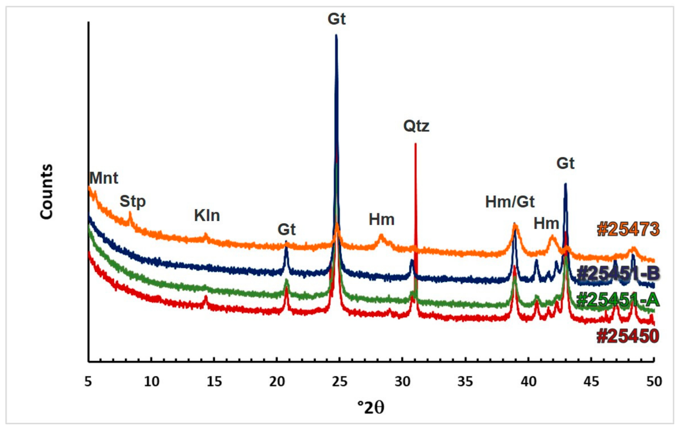
5.2. Whole Sample Mineral Identification

Mineral identification of whole-rock samples representing the three types of ferruginous materials was by X-ray Diffraction (XRD), optical microscopy, and Scanning Electron Microscopy (SEM). Powder-X-ray diffraction (XRD) data were collected using a Brucker D4 Endeavor AXS instrument operating with Co-Kα radiation. Data collection was from 5 to 90° 2θ. The XRD patterns were processed using Bruker DIFFRAC.EVA software.

As a check on the mineralogy of nodular and pisolitic material to ensure the suitability (i.e., presence of Fe oxide) of the material selected for (U–Th)/He-dating, shards of >300 μm-sized fragments from ferruginous nodules and pisoliths, amounting to 10–20 mg, were gently ground with 1–2 mL of ethanol in an agate mortar and pestle. The resulting slurry was pipetted onto a low-background, Si-holder and the ethanol allowed to evaporate, fixing the sample powder to the holder. Powder X-ray diffraction patterns were obtained on a Bruker D8 Discover diffractometer using Co Kα radiation (35 kV and 40 mA) and scanning from 5 to 80° 2θ in 0.015° 2θ steps, counting for 1.08 s/step for a total scan time of ≈90 min per scan. Displacement correction of diffraction patterns was made relative to quartz, acting as an internal standard, when detected.

Polished thin sections of ferruginous pisoliths and nodules were examined on a Zeiss Axiolmager petrographic polarizing microscope. Optical microscopy was followed by SEM-EDS analyses. Polished sections and the surfaces of freshly broken pisoliths and nodules were carbon/platinum coated and examined with a Zeiss Ultra–Plus field emission gun (FEG) SEM fitted with a semi-quantitative energy dispersive X-ray spectrometer (SEM-EDAX). An accelerating voltage of 20 kV with a beam current of 3 nA was used.

5.3. Whole Sample Chemical Analyses

Pulverized samples (N = 36) were digested in HF/multiacid aqua regia and heated to 180 °C in a closed Teflon crucible in a microwave (Anton Paar Multiwave PRO Microwave Reaction System) and were analyzed for the following elements by ICP-OES/MS (ppm detection limits in parentheses): Ag (0.01), Al (10), As (0.5), Ba (0.2), Be (0.2), Bi (0.1), Ca (10), Cd (0.05), Ce (0.05), Co (0.2), Cr (2), Cs (0.1), Cu (0.2), Dy (0.02), Er (0.05), Eu (0.02), Fe (100), Ga (0.05), Gd (0.05), Ge (0.05), Hf (0.02), Hg (0.05), Ho (0.02), In (0.01), K (10), La (0.05), Li (0.5), Lu (0.02), Mg (10), Mn (1), Mo (0.1), Na 910), Nb (0.5), Nd (0.02), Ni (2), P (5), Pb (0.2), Pr (0.05), Rb (0.1), Re (0.01), s (50), Sb (0.1), Sc (1), Se (0.05), Sm (0.02), Sn (0.2), Sr (0.1), Ta (0.01), Tb (0.02), Te (0.2), Th (0.02), Ti (10), Tl (0.1), Tm (0.05), U (0.02), V (2), W (0.1), Y (0.05), Yb (0.05), Zn (0.2) and Zr (1). Gold was analyzed by aqua regia digestion using 10–25 g of milled material and analyzed by ICP-OES/MS (Au 0.0001 ppm).

5.4. In Situ Chemical Analyses

In situ chemical analyses were performed on two polished thin sections by Tornedo (X-ray fluorescence) XRF (Bruker, Berlin, Germany) and Laser ablation ICP-MS (Teledyne CETAC (formally, PhotonMachines) - Omaha, NE, USA) to determine mineral element distributions and elemental associations in ferruginous nodules and pisoliths. The XRF maps were collected at the CSIRO laboratory in Perth using a Bruker M4 Tornado fitted with a Rh X-ray tube operating at 50 kV 500μA; data were collected at a pixel spacing of between 25 to 40 μm and a dwell time per pixel of 5 ms.

The trace elements were collected using a Photonmachines, ATLex 300si-x Excite 193 nm Excimer ArF laser connected to an Agilent 7700 ICP-MS (AGILENT TECHNOLOGIES inc, Santa Clara, CA, USA) located in the National Geosequestration Laboratory at CSIRO in Perth. The instrument was calibrated on NIST610 and NIST612 silicate glasses. The plasma conditions were optimized daily, to obtain the highest counts with oxide production (²⁴⁸ThO/²³²Th) remaining below 0.4%.

To create the maps, an 80 μm square beam was rastered from left to right across the sample at 60 μm/s [19] by the continuous movement of the stage under a fixed ablation site. At the start of each line, a 30-second analysis was collected with the laser off as a background. After 15 lines, a block of standard reference materials was analyzed. The following isotopes were measured in this study: Al²⁷, Si²⁹, S³⁴, Ti⁴⁷, V⁵¹, Cr⁵², Mn⁵⁵, Fe⁵⁷, Cu⁶³, As⁷⁵, In¹¹⁵, Sn¹¹⁸, Sb¹²¹, and Au¹⁹⁷ with a total combined sampling time of 0.141 s for all isotopes.

The certified reference material was NIST610 glass with UQAC FeS-1 used as a secondary standard as it has similar ablation characteristics as the sample. Data were reduced using Iolite software (software version 5.3, The University of Melbourne, Melbourne, Australia) [20] with the semi-quantitative method. Using this method, we achieved a precision of ~9% and accuracy within 10% for Si, Ti, V, Cr, Mn, and Fe.

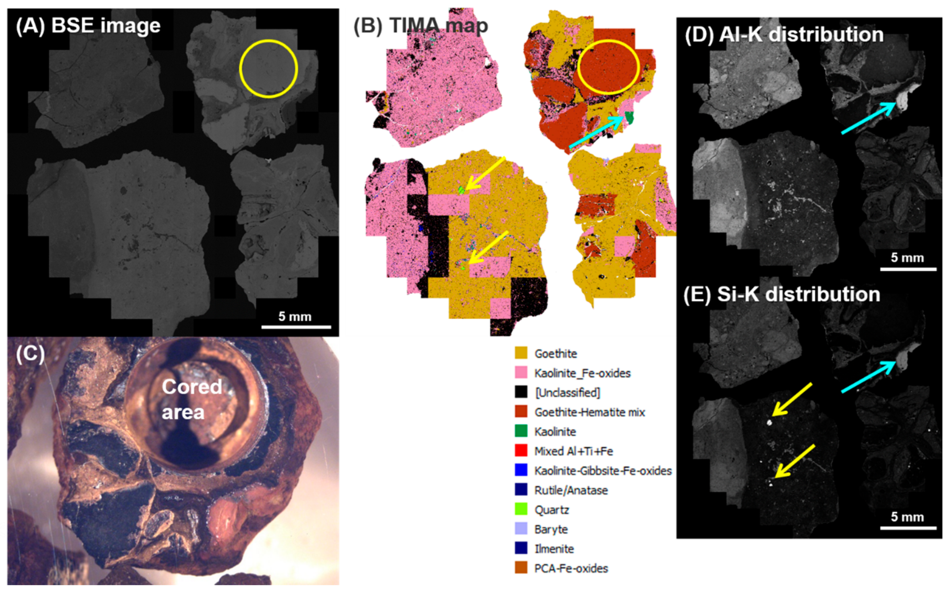
5.5. TIMA Mineral Mapping of Selected Samples for Dating

Bulk mineral characterization of samples representative of the three ferruginous nodules and pisolith types formed the basis of selecting samples for dating. Polished mounts (25 mm in diameter) of the basal zone of the Wollubar Sandstone (NWS, #25450, depth 31–32 m), the middle zone of the Perkolilli Shale (PPS, #25451, depth 16–18 m), and the flank of the paleochannel formed from weathered saprolite (NSP, #25473, depth 13–14 m) were prepared for in situ mineralogical characterizations by optical microscopy and SEM mineral mapping. Combined mineral and elemental mapping of three samples of ferruginous nodules and pisoliths was achieved with a TESCAN Integrated Mineral Analyzer (TIMA; Tescan Orsay Holding, Brno, Czech Republic) using the method of [21]. The TIMA is a scanning electron microscope (SEM) equipped with four silicon drift, energy dispersive X-ray spectrometers (EDS). Mineral analysis was conducted using the DOT mode of the TIMA [22], with operating conditions of 25 kV beam voltage, 85.0 nm spot size, 15 mm working distance, and an imaging field size of 1500 × 1500 μm. During scanning, a backscattered electron (BSE) image was collected at a 3 μm resolution and used to determine the boundaries between mineral grains. An EDS spectrum was acquired at a grid-spacing of 20 μm. Composite mineral distribution maps were then generated by comparing the measured mineral EDS signature to an in-house, standardized regolith EDS mineral library with mineralogy verified by Raman and XRD data (e.g., [3]). XRD mineralogy was used to validate the TIMA mineral-mapping library used to generate mineral distribution maps and to constrain the TIMA mineralogy identified, particularly where phases or mineral mixtures, such as Fe oxides and clays, may have a similar (EDS) composition.

5.6. (U–Th)/He Dating

Regions of interest (ROIs) within ferruginous nodules and pisoliths, identified as suitable (goethite-rich) for (U–Th)/He dating on the basis of the TIMA mineral mapping and following the sample selection criteria described by [3], were subsampled using a diamond drill to extract cores measuring 3 mm in diameter and 3–5 mm in length. Cores from each ferruginous nodule and pisolith were crushed and sieved to recover fragments of the 200–300 μm size fraction. Following ultrasonic cleaning in ethanol, five replicates of each sample were prepared by hand-picking, under an optical microscope, of texturally homogeneous fragments. These were loaded into Nb tubes prior to He extraction. The large size of the fragments, comprising aggregates of typically <1 μm sized Fe oxide crystals, eliminates the effect of alpha ejection and potential diffusive loss of ⁴He, which can be a source of error in applications of (U–Th)/He dating (e.g., [2]).

The (U–Th)/He analyses were conducted at the Low-Temperature Thermochronology Facility at the John de Laeter Centre (Curtin University, Perth) following the analytical procedures of [23], as summarized by [3]: Nb-tubes containing the Fe-rich fragments were loaded into an ultra-high vacuum extraction line and degassed in a single, 10-minute heating cycle at ~450 °C using a diode laser to circumvent possible changes in the composition of the parent isotopes, such as the potential loss of U that may occur at much higher (e.g., >1100 °C) extraction temperatures [23]. Initial test work prior to analysis confirmed that this degassing method resulted in the complete outgassing of the samples without the need to ‘re-extract’. Evolved gas was purified using a ‘cold finger’ cooled with liquid nitrogen and a hot (~350 °C) Ti–Zr getter, spiked with 99.9% pure ³He, and introduced into a Pfeiffer Prisma QMS-200 mass spectrometer, next to a cold Ti–Zr getter. The ⁴He/³He ratios, corrected for HD and 3H by monitoring mass 1, were measured by a Channeltron detector operated in static mode. Evolved ⁴He contents (measured in nano-cubic centimeters, ncc) were determined by isotope dilution using a ³He spike against calibrated ⁴He gas standards, with empty Nb-tubes heated using the same procedure for blank correction.

Following the ⁴He measurements, the Nb-tubes containing the samples were retrieved from the laser cell, spiked with ²³⁰Th and ²³⁵U, and dissolved in 200 μL of concentrated HCl in Parr bombs heated to 210 °C for 30 h. Each Parr bomb also contained blank and spiked standard solutions. All solutions were analyzed for U and Th on an Agilent 7500 ICP-MS at TSW Analytical Ltd. (University of Western Australia, Perth) using an Agilent 7500 ICP-MS. The total analytical uncertainty (TAU) values of 3.1–5.5% were calculated as the square root of the He analysis uncertainty and weighted uncertainties of the U and Th measurements [23]. Measured (U–Th)/He-dates were not corrected for alpha ejection or diffusive loss due to the polycrystalline nature and large size of the measured fragments (e.g., [2,23]).

6. Results

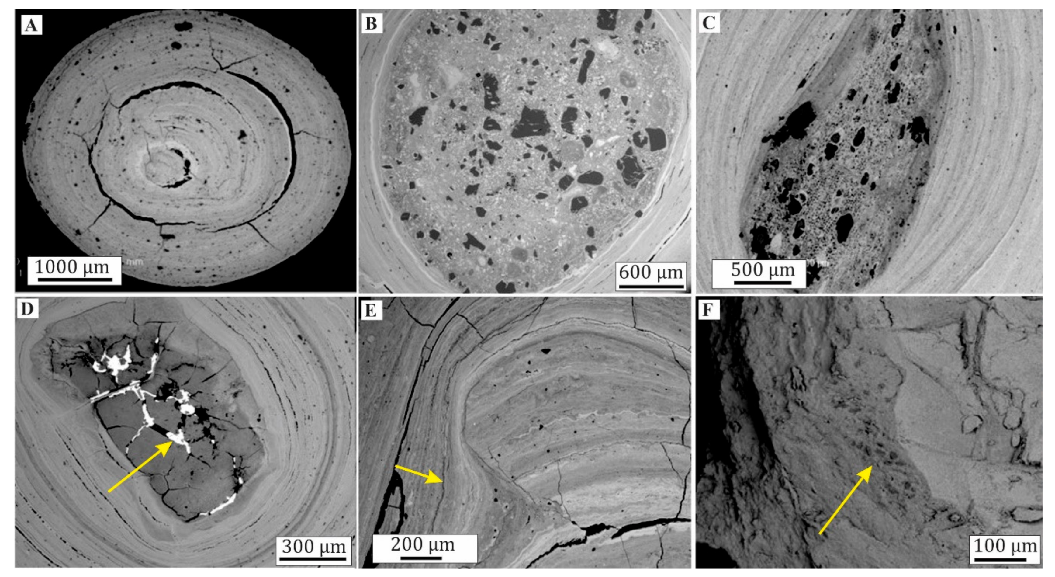
6.1. Ferruginous Pisoliths in the Perkolilli Shale (PPS)

Pisoliths randomly distributed in the Perkolilli Shale are yellow to brown, range in diameter from 2 to 15 mm with the majority being between 2 to 6 mm and have high sphericity with smooth outer surfaces (Figure 6A). Pisoliths typically have well-developed, goethite-rich, multiple laminae that extend to the center of the pisolith (Figure 6A) or encase a nucleus of quartz (Figure 6B), goethite-replaced wood fragments (Figure 6C), or ferruginous clay to sandy clay (Figure 6D). Some pisoliths seem to lack a nucleus, although this could be due to having not sectioned the pisoliths through its centre. Ferruginized clay is predominantly composed of kaolinite and goethite.

Pisoliths contain a variety of structures that show biological influence during pisolith formation. The most obvious is the ferruginized wood nucleus common to many pisoliths (Figure 6C). The nucleus in these samples was up to 2 mm across and was often preserved by goethite and display mimetic textures in which only the cell tissue is replaced, leaving the porosity defined by the xylem and phloem vessels (Figure 6C). SEM observation of the internal surfaces of the woody materials reveals ferruginized microfossils (Figure 7A,B) in a matrix of acicular and radial crystals of goethite (Figure 7B,C). The tubular ferruginized microfossils bear a marked resemblance to the fungi and bacteria preserved by Fe oxides within pisoliths, nodules, and concretions [9,24]. Such pisolith morphologies show similar morphology to pisoliths described in earlier work [1,9,17]. Similarly preserved wood fragments were reported in other Fe-rich environments, such as in the Pilbara Channel Iron Deposits (CID) (e.g., [25]) that formed either through the pedogenic alteration of wood/charcoal fragments later deposited in the accumulating CID and/or via in situ replacement of wood/charcoal fragments within the consolidating CID [26].

The number of goethite laminae in the cortices of pisoliths varies greatly, depending upon the grain size, but generally, there are 20 or more laminae forming the bulk of the pisolith (Figure 6). However, in larger pisoliths (>8 mm), cortical laminae of goethite are well developed but generally thin (<2 mm). In places, barite infills cracks (Figure 6D). SEM examination of the internal surface of cortices show oriented acicular crystals of goethite (Figure 7D). Only the first few cortices closely follow the small external irregularities of the nucleus; the cortices become more and more regular and circular outwards as irregularities are progressively infilled. Discordant boundaries or micro-unconformities occur between some sets of cortical laminae, as do thin laminae of silt-sized quartz (Figure 6E,F). Accretionary growth of these layers creates the banded structure characteristic of pisoliths of the paleochannel. The boundary between the nucleus and the surrounding cortex is generally sharp.

6.2. Ferruginous Nodules in the Wollubar Sandstone (NWS) and in Saprolite (NSP)

The nodules NWS and NSP, are much simpler in appearance and larger than the ferruginous pisoliths (Figure 5). They are homogeneous, yellowish to dark-reddish brown, irregular and up to 50 mm across, with the majority being between 10–20 mm. They may have a thin, <1 mm cortex of goethite (Figure 5). The nucleus-to-cortex ratio is much greater in nodules where the cortex comprises <5% of the nodules as a whole compared to the PPS, where the cortex may make up more than 90% of the pisolith. Manganese coatings are common on the surface of NWS (Figure 5). Quartz grains in NWS are subangular to subrounded, 20–100 μm in size, and are mainly cemented by platy and botryoidal goethite (Figure 8A,B). Needle-shaped crystals of chromite fill the cracks and voids (Figure 8A,B). In NSP, 2–5 μm tubular crystals of halloysite, platy (0.5–2 μm) crystals of kaolinite, and aggregates of spherical and platy crystals of goethite and hematite form the matrix of the core (Figure 8D).

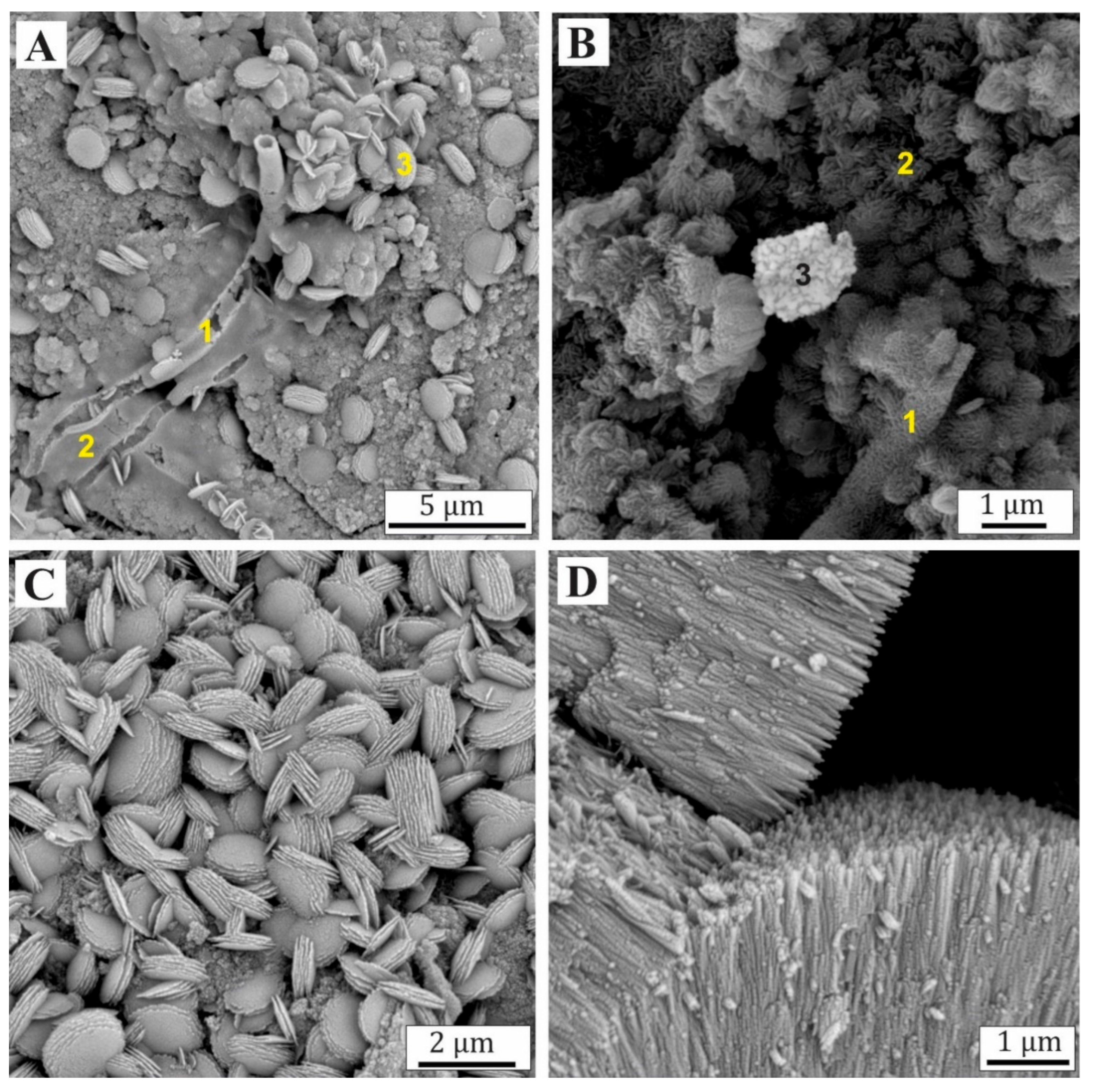
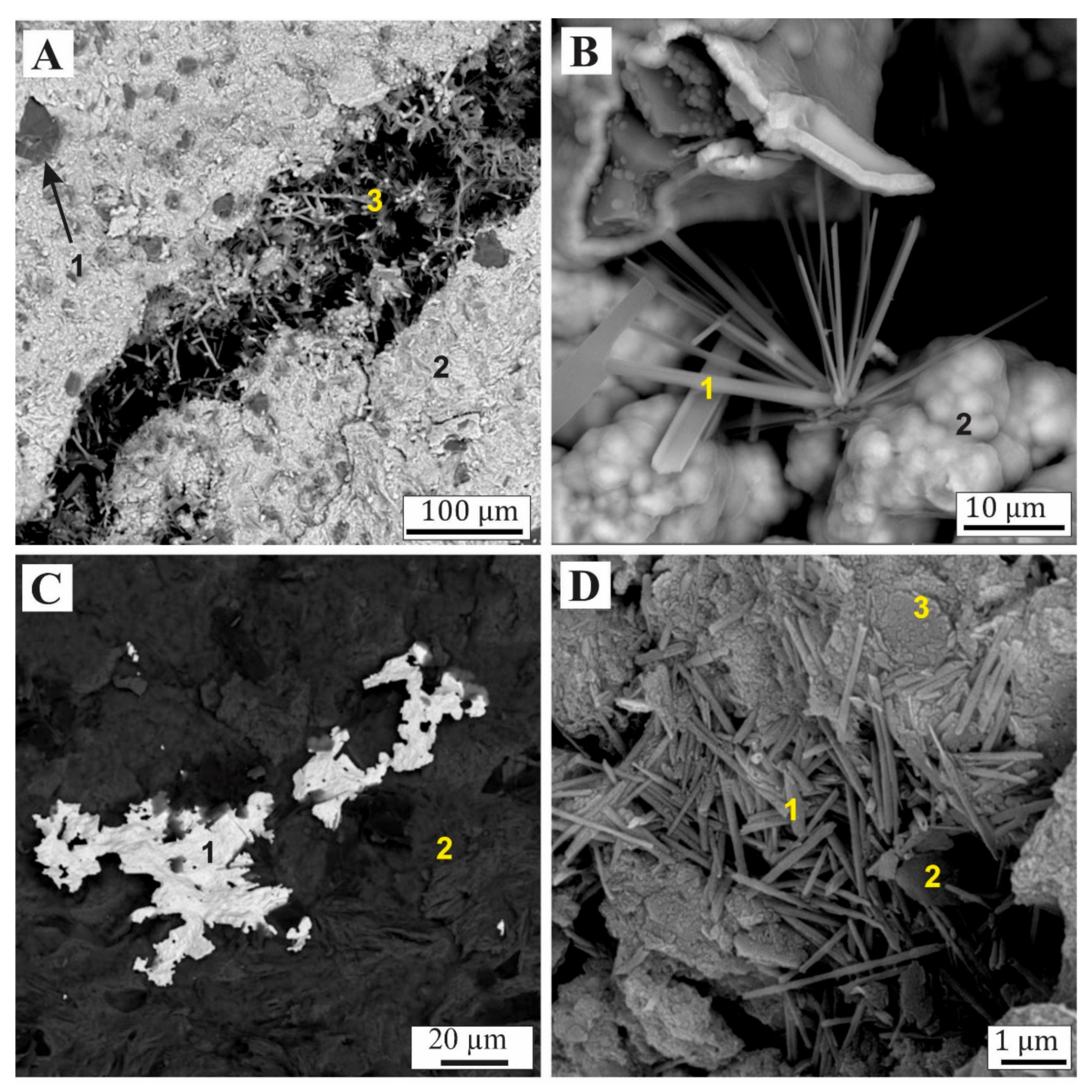
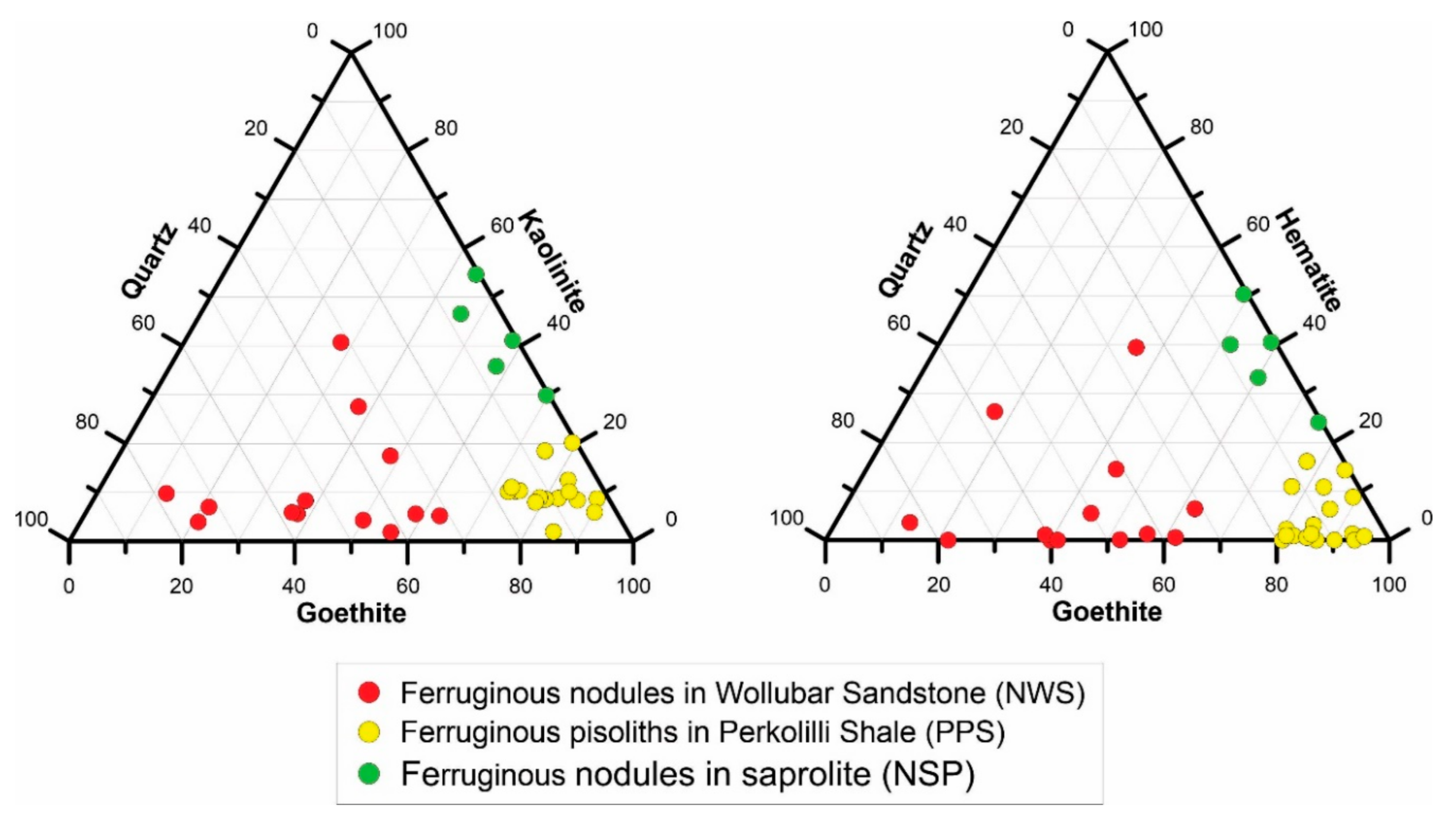
6.3. Mineralogical Differentiation of Ferruginous Nodules and Pisoliths

The relative abundance of goethite, hematite, quartz, and kaolinite in whole samples varies according to the origin of ferruginous materials (Figure 9). The PPS are typically goethite-rich with very small amounts of hematite, kaolinite, and quartz. In contrast, the NWS are dominated by variable amounts of quartz and goethite with small amounts of hematite and kaolinite, consistent with their formation from the Wollubar sandstone. The NSP are dominated by kaolinite, hematite, and goethite with very low quartz. Gibbsite (up to 18 wt %) and small amounts (<5 wt %) of talc occur in some samples of the NSP. The presence of talc and abundant kaolinite and very little or no quartz in the NSP reflects their formation from the weathering of ultramafic bedrock. The presence of gibbsite in the NSP indicates well-drained environments on the flanks of the paleochannel. Goethite being the dominant mineral in the NWS and PPS suggest its formation in hydromorphic environments whereas hematite in the NSP is formed by the dehydration of goethite in an oxidizing environment, it can also form directly by internal dehydration of ferrihydrite [27].

XRF mapping provided in situ information for some elements in the PPS and NWS. The XRF mapper data for the PPS show Fe and Al, with Fe being dominant in varying concentrations in alternating lamina surrounding the nucleus of the PPS (Figure 10). Silica occurs as discrete quartz grains, and Si and Al occur as kaolinite in some cores. In the NWS, Fe is almost uniformly distributed throughout the core whereas Si occurs as quartz grains (Figure 11). Spots of Cr, Ti (Figure 10), and V (not shown) occur in many cores of the PPS but generally not in the laminae. In contrast, in the NWS, Cr (not shown) and Ti are almost uniformly distributed throughout the core matrix whereas, Mn occurs in veins and fractures (Figure 11) that were probably deposited after pisolith formation. Samples of the NSP were not investigated by the Tornado XRF mapper.

6.4. Whole-Rock Geochemistry of Selected Ore-Related Elements in the PPS, NWS and NSP

Summary statistics of selected ore-related elements for the PPS and NWS is shown in

Table 1. Summary statistics of selected elements for the PPS and NWS.

	PPS over Mineralization (N = 11)				PPS over Background (N = 7)
Element	Min	Max	Mean	Median	Min	Max	Mean	Median
As-ppm	151	1340	330	280	66	129	97	87
Au-ppb	4	436	124	68	1	16.6	6.9	6.4
Bi-ppm	0.6	2.6	1.3	1.2	0.4	0.7	0.48	0.5
Cu-ppm	97	381	170	142	52	86	66	63
In-ppm	0.1	0.2	0.16	0.16	0.09	0.14	0.11	0.1
S-ppm	785	1310	1014	1020	147	505	323	336
Sb-ppm	3	5.9	4.3	4.2	2.3	5.6	3.5	3
Se-ppm	1.98	4.66	3.39	3.42	1.05	1.58	1.35	1.3
	NWS over Mineralization (N = 9)					NWS over Background (N = 4)
Element	Min	Max	Mean	Median	Min	Max	Mean	Median
As-ppm	33	5480	1124	470	90	1520	536	268
Au-ppb	6.6	11,700	2679	515	3.6	55.4	21.7	14
Bi-ppm	0.05	2.9	0.95	0.8	0.1	0.3	0.17	0.1
Cu-ppm	37	1741	401	249	49	159	84	64
In-ppm	0.06	0.24	0.15	0.12	0.02	0.04	0.03	0.03
S-ppm	201	715	455	456	25	226	131	136
Sb-ppm	2	8	3.7	3.1	0.4	2.6	1.3	1
Se-ppm	1	15.7	4.04	1.85	0.55	0.78	0.65	0.64

and the distribution of Au, In, S, Se, As, Cu, Bi, and Sb over mineralization and background is shown in Figure 12 and Figure 13. The whole rock geochemistry of the PPS over mineralization shows multi-element anomalies in Au (median 68 ppb, maximum 436 ppb), As (median 280 ppm, maximum 1340 ppm, Bi (median 1.2 ppm, maximum 2.6 ppm), Cu (median 142 ppm, maximum 381 ppm), In (median 0.16 ppm, maximum 0.2 ppm), S (median 1020 ppm, maximum 1310 ppm), Sb (median 4.2 ppm, maximum 5.9 ppm) and Se (median 3.42 ppm, maximum 4.66 ppm). These elements are significantly more abundant over mineralization compared to background samples (Table 1, Figure 12 and Figure 13).

The same suite of elements is also anomalous in the NWS with significantly higher concentrations compared to the PPS for Au, As, Bi, and Cu (Table 1). Arsenic dispersion is greater reaching 1520 ppm in the background area. Sulfur, In, Sb, Pb, and Se concentrations are less in the NWS compared to the PPS. Anomalous elements include Au (median 515 ppb, maximum 11700 ppb), As (median 470 ppm, maximum 5480 ppm), Bi (median 0.8 ppm, maximum 2.9 ppm), Cu (median 249 ppm, maximum 1741 ppm), In (median 0.12 ppm, maximum 0.24 ppm), S (median 456 ppm, maximum 715 ppm), Sb (median 3.1 ppm, maximum 8 ppm) and Se (median 1.85 ppm, maximum 15. 7 ppm). The concentrations of ore-related elements are relatively low in the NSP compared to the NWS and PPS. These include Au (median 7.6 ppb, maximum 32 ppb), As (median 329 ppm, maximum 405 ppm), Bi (median 0.7 ppm; maximum 1.6 ppm, Cu (median 54 ppm, maximum 69 ppm), In (median 0.18 ppm, maximum 0.19 ppm), S (median 504 ppm, maximum 761 ppm), Sb (median 3.5 ppm, maximum 3.6 ppm) and Se (median 1.9 ppm, maximum 2.2 ppm)

Visible Au occurs both in the NWS and PPS, being more common in the NWS. This visible Au varies in size from 0.1 to 20 μm and is confined to cavities and the matrix of nodules and pisoliths (Figure 7B and Figure 8C). Authigenic Au typically contains no Ag and is secondary.

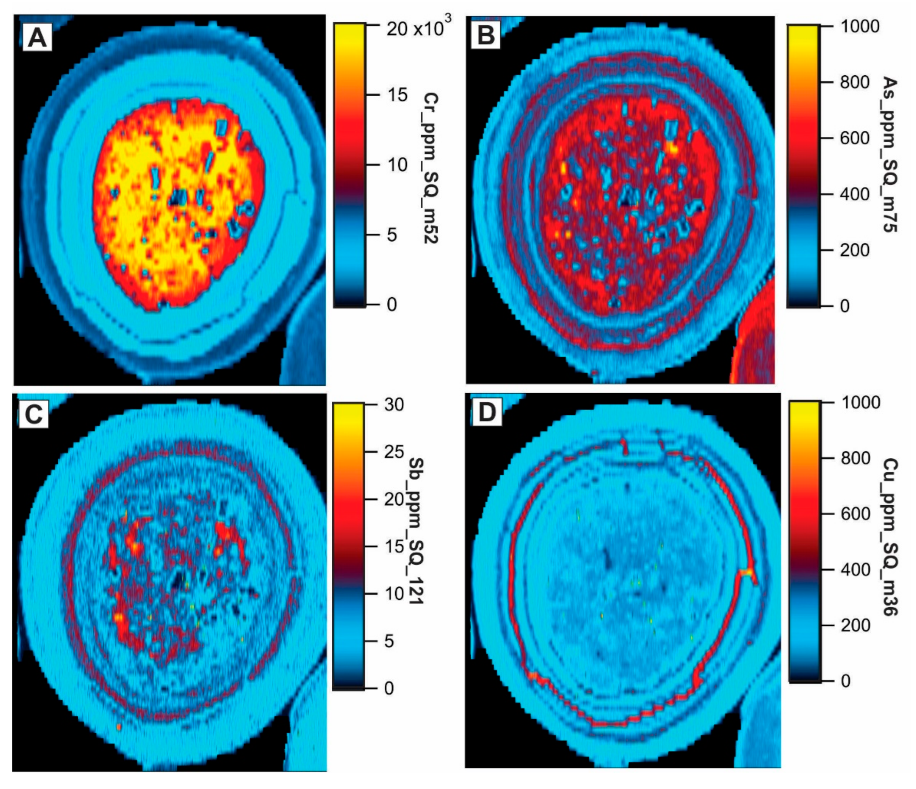
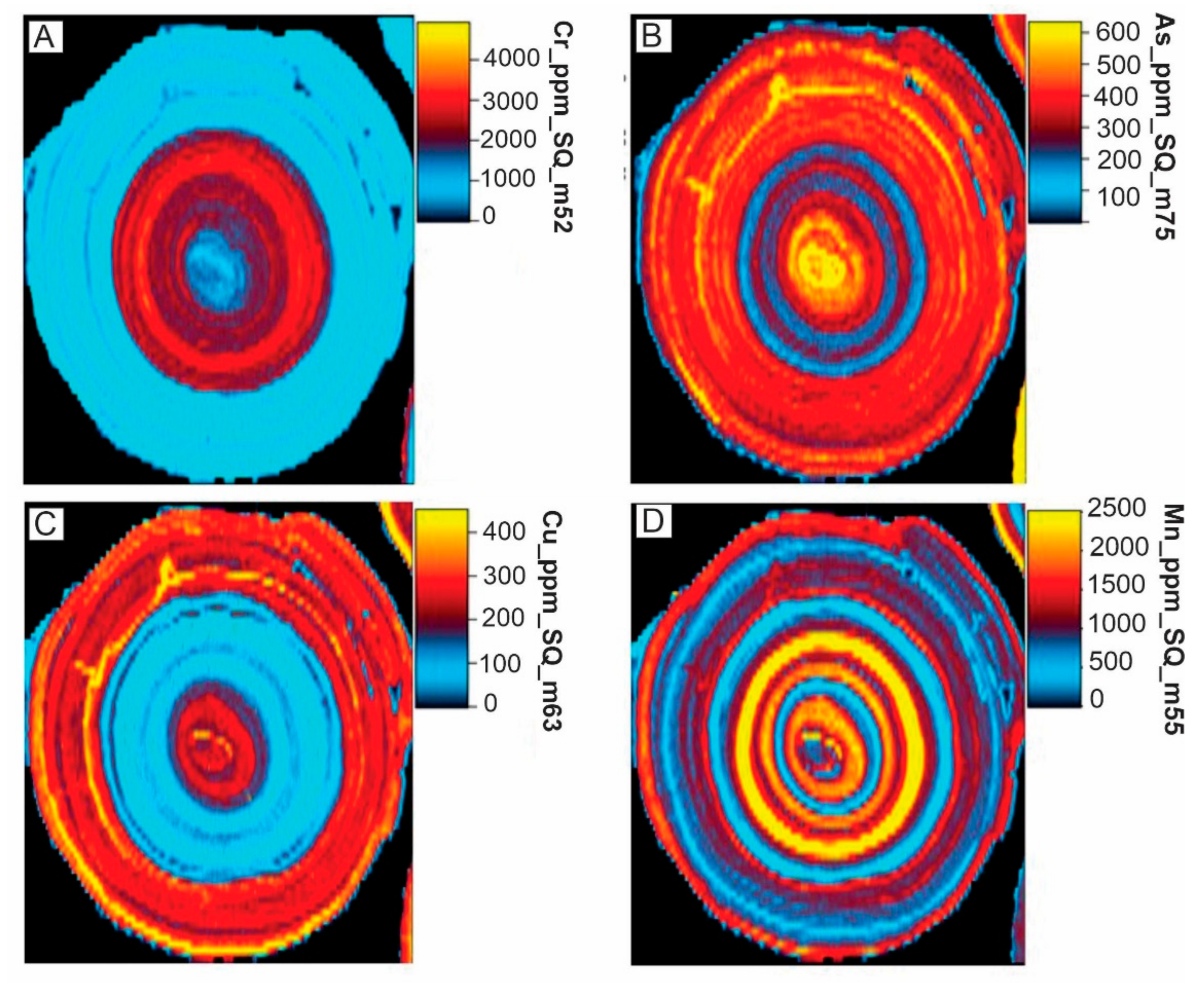
6.5. Laser Ablation ICP-MS Mapping of Elements

Laser ablation ICP-MS permits trace element chemistry on a finer scale than the XRF mapper (Figure 14, Figure 15 and Figure 16). Three individual pisoliths from the PPS sample and one nodule from the NWS were investigated by Laser Ablation ICP-MS. The PPS 1 and 2 have small cores with many goethite-rich laminae (approximately 5 mm) whereas, PPS 3 has a larger core with very thin laminae (approximately 10 mm). The NWS has no or a very thin cortex. Some of the results are shown in Figure 14, Figure 15 and Figure 16. The general trends are:

In PPS 1, Cr, As, Sb (Figure 14A–C), V, Sn, and Ti are concentrated in the core with some As, Sb in a few inner laminae. Copper and Mn occur in a few laminae only and Fe in both core and all laminae. Chromium, V, Ti, Sn, As, Sb, and Al occur in the core and are strongly correlated with each other and Al (r = 0.5 to 0.83) but not with Fe, suggesting a common host for these metals probably a detrital metal-rich, clayey, weathered mineralized fragment. A strong positive correlation between Fe and Cu (r = 0.66), Fe and As (r = 0.47), and Mn and Cu (r = 0.71) suggests an association of As with goethite and Cu with both Fe and Mn oxides that make up a large proportion of the laminae.

In the PPS 2 (Figure 15), except Cr in the core, there is a significant dispersion of As, Cu, and Mn in both laminae and in the core (Figure 15). Iron appears to control to some extent the distribution of As (r = 0.29) but Cu distribution is not controlled by Fe as there is a negative correlation between Fe and Cu (r = −0.23). Copper and As are strongly correlated with V (V vs. Cu, r = 0.69; V vs. As, r = 0.67), indicating their similar behavior.

In PPS 3 (not shown), Cr is confined to the core, V, Fe, Mn, As, and Cu are dispersed in laminae. Gold occurs as veins in the core. Here, due to a significant correlation between Al and Cr (r = 0.54), Cr appears to be hosted in a metal-rich weathered mineralized fragment whereas the strong correlation between Fe and V (0.57), Fe and Cu (r = 0.82) and Fe, and As (r = 0.83) suggest their association with goethite.

In the NWS, Cr, Au, As, and Cu (Figure 16) occur in veins and fractures whereas S, is uniformly distributed throughout the core matrix. Strong correlations between Fe and Cu (r = 0.69), Fe and As (r = 0.72), Fe and V (r = 0.67), Fe and S (r = 0.61) indicate their association with goethite.

The PPS show a variety of elemental distributions highlighting that each pisolith is different with more than one mineral hosting the trace elements. In contrast, element distribution patterns in NWS nodules are more consistent. However, it is also worth pointing out that trace elements to Fe ratios vary for both types of ferruginous nodules and pisoliths. For example, in the PPS1, As/Fe, Cu/Fe, and Cr/Fe ratios are higher in the core compared to the laminae. In summary, there is physical dispersion of metal-rich, weathered mineralized fragments in the cores, whereas hydromorphic dispersion occurs in goethite that forms the laminae of pisoliths.

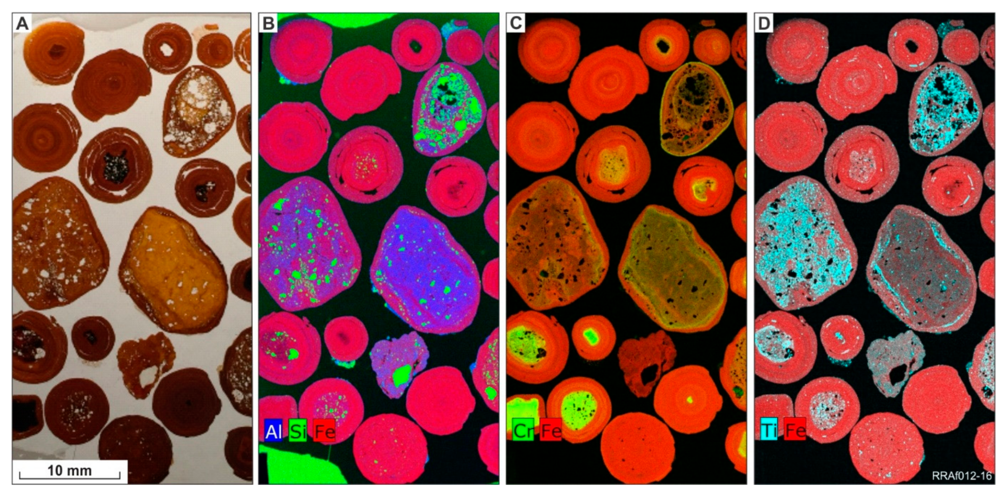
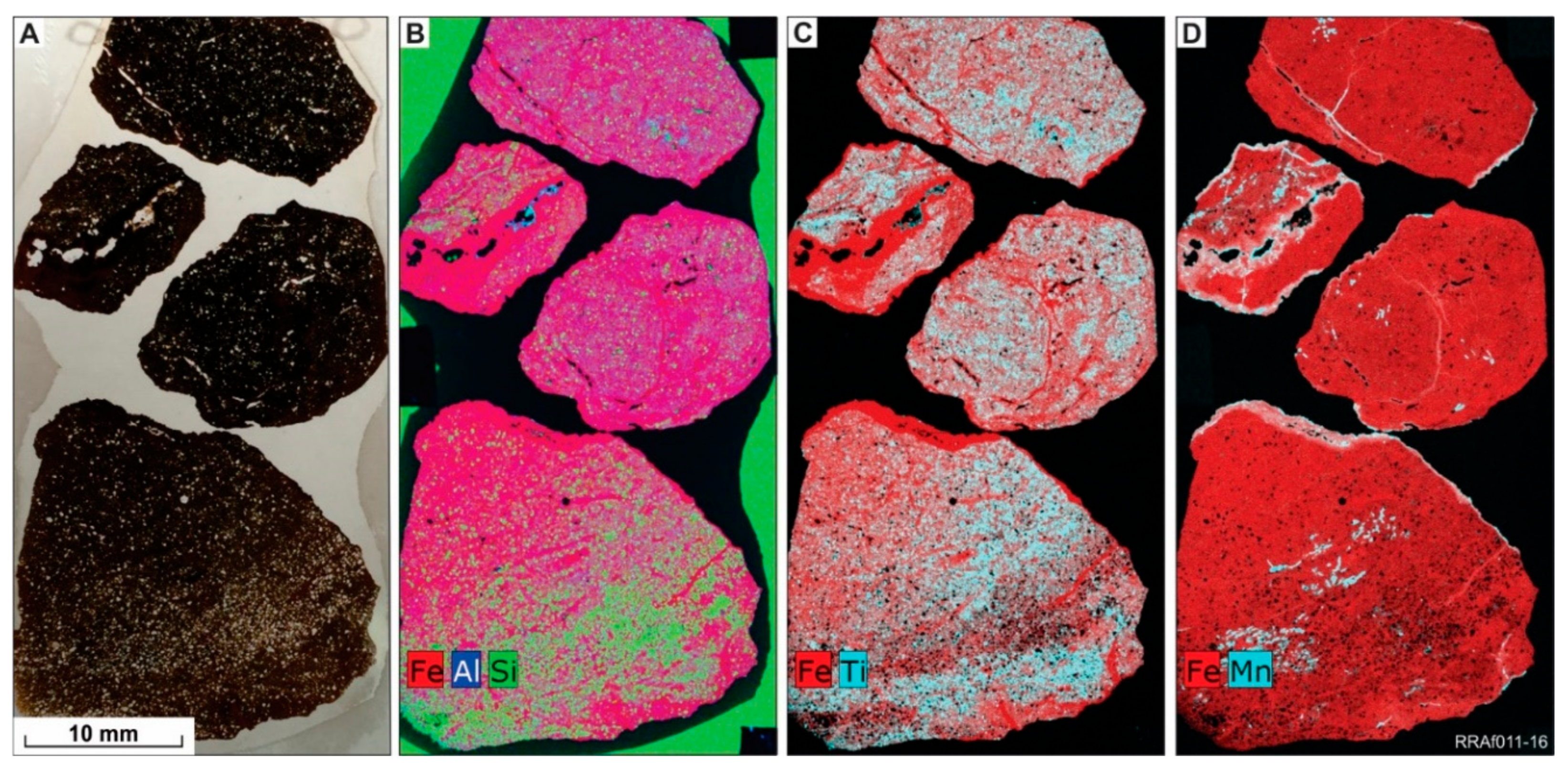
6.6. Mineralogy of Dated Samples

XRD analysis of the >300 μm fraction for each sample (Figure 17) confirmed the Fe oxide-rich nature of the ferruginous nodules and pisoliths with those of the NSP (#25473,

Table 2. XRD mineralogy of the >300 μm fraction of cored material from ferruginous nodules and pisoliths from drill core material selected for (U-Th)/He-dating. maj=major; Tr=trace; min=minor.

Sample	Mineralogy
NSP (#25473)	Hematite, goethite (maj); kaolinite, stilpnomelane, smectite (min)
NWS (#25450)	Goethite (maj); quartz (min); kaolinite, paragonite (tr)
PPS (#25451-A)	Goethite (maj); quartz (tr)
PPS (#25451-B)	Goethite (maj)

) containing both goethite and hematite, compared to the NWS (#25450) and the PPS (#25451), which contained only goethite as the predominant Fe-bearing phase (Table 2). The NSP and NWS have more varied mineralogy compared to the PPS (Table 2). The small amounts of kaolinite and smectite detected (Table 2) most likely formed from the weathering of included, primary alumino-silicates.

TIMA back-scatted (BSE) images and false-color mineral maps, with mineralogy verified by XRD analysis, for each sample examined in the study are shown in Figure 18, Figure 19 and Figure 20. TIMA mineral mapping better highlights the mineral and textural complexity than can be discerned solely from BSE imaging (Figure 18, Figure 19 and Figure 20). The NSP (#25473) and NWS (#25450) samples are more nodular in appearance having irregular shapes and embayments (e.g., Figure 18A and Figure 20A), compared to the spherical pisoliths from the PPS (#25451) (Figure 19). Many PPS pisoliths display a conspicuous, concentric ‘onion-ring’ structure with well-developed cortices.

Elemental mapping of the Al and Si distribution enables a more efficient means of phase identification, particularly for phases or mineral mixtures that may have a similar BSE contrast, and provides an accurate indication of the mineralogical complexity that can occur in ferruginous nodules and pisoliths. Co-incidentally bright (i.e., white), high-contrast areas in Al-K and Si-K maps indicate the presence of clay (e.g., kaolinite), as mapped in #25473 (Figure 19B,D,E). Bright (i.e., white), high-contrast ‘specks’ in Si-K distribution maps indicate the presence of quartz, for example, in NWS (#25450), which shows an abundance of quartz grains cemented by goethite (Figure 20E).

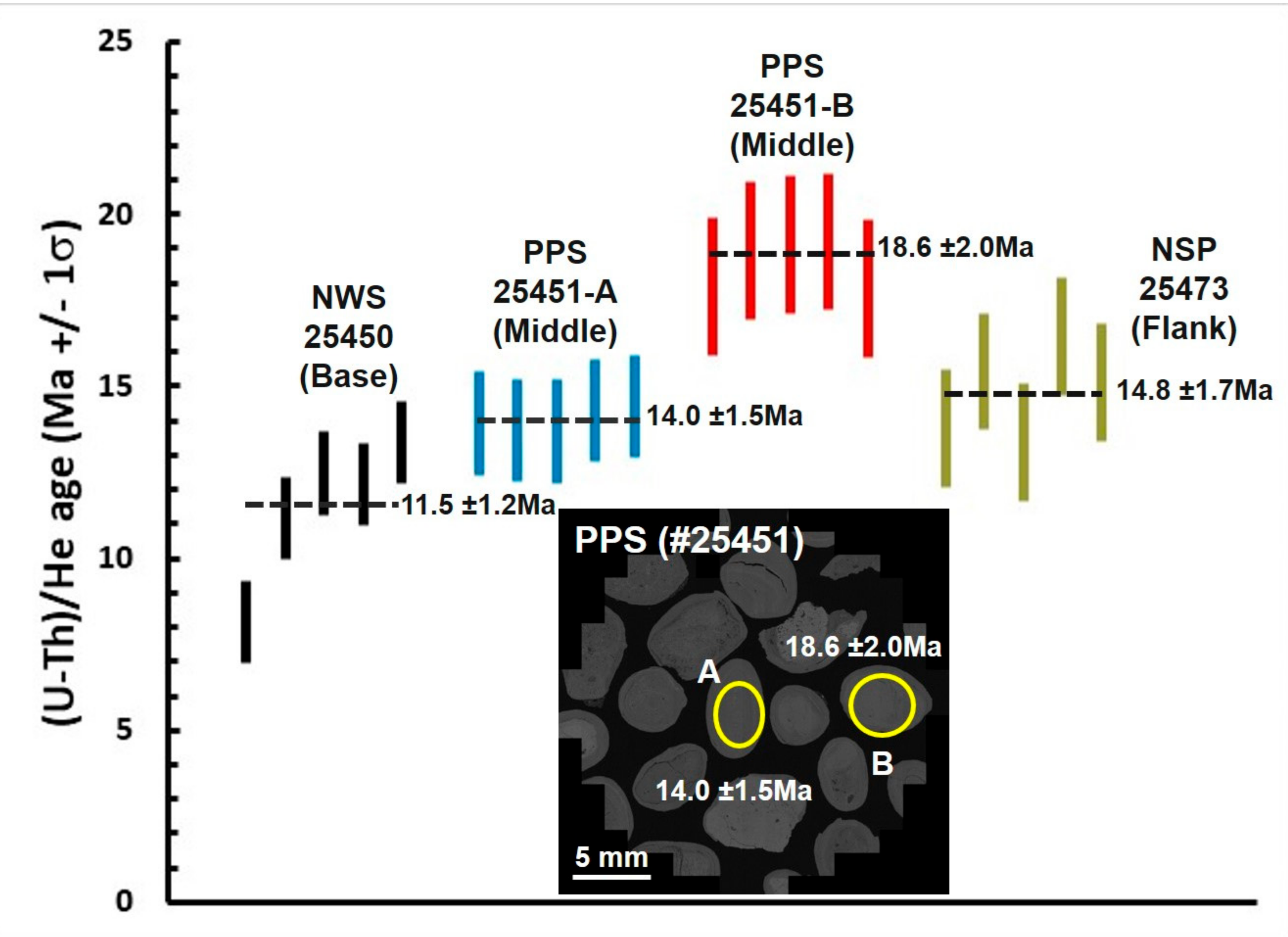
6.7. (U–Th)/He Dating

Raw and corrected (U–Th)/He replicate ages and measured U, Th, and He contents for goethite-rich, NWS, PPS, and NSP samples are presented in

Table 3. Dating results for all sample replicates, with the calculated average (U–Th)/He age and error for each sample highlighted in grey.

Sample	232Th	±	238U	±	He	±	TAU#	Th/U	Raw Age	±1σ	Ft	±	Cor. Age	±1σ
Code	(ng)*	(%)	(ng)	(%)	(ncc)^	(%)	(%)		(Ma)	(Ma)		(%)	(Ma)	(Ma)
NWS
25450-1	0.010	2.5	0.079	2.8	0.081	3.3	4.3	0.13	8.2	0.3	1.00	10	8.2	0.9
25450-2	0.007	5.7	0.110	2.2	0.151	2.7	3.5	0.07	11.2	0.4	1.00	10	11.2	1.2
25450-3	0.012	4.2	0.116	2.2	0.181	2.6	3.4	0.10	12.5	0.4	1.00	10	12.5	1.3
25450-4	0.006	8.3	0.105	2.3	0.157	2.7	3.5	0.05	12.1	0.4	1.00	10	12.1	1.3
25450-5	0.003	2.5	0.055	2.8	0.091	3.0	4.1	0.05	13.4	0.6	1.00	10	13.4	1.4
													11.5	1.2
PPS
25451-A-1	0.192	1.7	0.328	2.3	0.634	2.5	3.2	0.58	13.9	0.4	1.00	10	13.9	1.5
25451-A-2	0.361	1.7	0.422	2.2	0.848	2.5	3.1	0.85	13.7	0.4	1.00	10	13.7	1.4
25451-A-3	0.451	1.7	0.677	2.2	1.305	2.5	3.2	0.66	13.7	0.4	1.00	10	13.7	1.4
25451-A-4	0.702	2.5	0.687	2.8	1.484	2.4	3.3	1.02	14.3	0.5	1.00	10	14.3	1.5
25451-A-5	0.679	1.7	0.669	2.3	1.455	2.5	3.1	1.01	14.4	0.5	1.00	10	14.4	1.5
													14.0	1.5
PPS
25451-B-1	0.053	2.0	0.417	2.3	0.936	2.5	3.3	0.13	17.9	0.6	1.00	10	17.9	1.9
25451-B-2	0.104	1.8	0.254	2.2	0.642	2.5	3.2	0.41	19.0	0.6	1.00	10	19.0	2.0
25451-B-3	0.033	2.6	0.231	2.8	0.557	2.6	3.8	0.14	19.1	0.7	1.00	10	19.1	2.0
25451-B-4	0.118	1.8	0.364	2.2	0.917	2.5	3.2	0.32	19.2	0.6	1.00	10	19.2	2.0
25451-B-5	0.048	2.0	0.405	2.3	0.904	2.5	3.3	0.12	17.8	0.6	1.00	10	17.8	1.9
													18.6	2.0
NSP
25473-1	0.203	1.7	0.073	2.3	0.203	5.0	5.3	2.75	13.8	0.7	1.00	10	13.8	1.6
25473-2	0.196	2.4	0.052	2.8	0.185	5.1	5.5	3.74	15.4	0.8	1.00	10	15.4	1.8
25473-3	0.122	1.8	0.038	2.6	0.108	5.2	5.4	3.23	13.4	0.7	1.00	10	13.4	1.5
25473-4	0.084	1.8	0.096	2.3	0.232	5.0	5.4	0.87	16.5	0.9	1.00	10	16.5	1.9
25473-5	0.063	1.9	0.196	2.3	0.387	4.9	5.3	0.32	15.1	0.8	1.00	10	15.1	1.7
													14.8	1.7

. Averaged (U–Th)/He ages of 18.6–11.5 Ma for all ferruginous nodules and pisoliths indicate a mid-Miocene age (Table 3). These may be compared to the (U–Th)/He ages of 10.0–7.5 Ma of ferruginous pisolitic and fragmental duricrusts from Morangup Hill, in the western Yilgarn Craton near Toodyay [2]. Significantly younger, late-Miocene/Pliocene to possible early-Pleistocene (U–Th)/He ages of 5.8–1.3 Ma were determined on pisoliths and fragmental duricrust nodules from the Boddington Au mine, also in the western Yilgarn Craton, southeast of Perth [3].

There are significant differences in the ages for the three types of samples. Corrected (U–Th)/He ages for the PPS (16–18 m depth) ranged from 13.7 ±1.4 Ma to 19.2±2.0, for the NWS (31–32 m depth) ranged from 8.2 ± 0.9 to 13.4 ±1.4 Ma and for the NSP (13–14 m depth) ranged from 13.4 ±1.5 Ma to 16.5 ±1.9 Ma. It is interesting to note a significant difference in the (U-Th)/He ages for individual PPS (Figure 21), suggesting a complex and prolonged genesis with pisolith formation occurring over a period of several (4–5) million years. Corrected ages, ranged from ca. 19 Ma for the PPS in the middle of the paleochannel to ca. 8 Ma for the NWS at the bottom of the paleochannel, indicating diachronous ferruginization of the aggraded channels. These findings are similar to those reported for goethite dated in the Yandi paleochannel in the Hamersley Province of Western Australia by [29], where (U–Th)/He ages for goethite ranged from ca. 18 Ma near the surface to ca. 5 Ma at the bottom of the profile. It is important to note that the measured (U–Th)/He ages relate only to the formation of individual pisoliths and not to deposition of the paleochannel. A ranked-order plot of the ferruginous nodules and pisoliths (U–Th)/He ages demonstrates the relative age differences within and between individual paleochannel samples and the range in the (U–Th)/He ages measured in each case (Figure 21).

7. Discussion

7.1. Formation of Ferruginous Nodules and Pisoliths and Landscape Evolution

The combination of dating, geochemical and mineralogical data from the paleochannel and associated ferruginous nodules and pisoliths provides a comprehensive view of the environment in which the landscape at Garden Well has evolved. Summary of dating and geochemical dispersion in various regolith materials is shown in Figure 22. Three types of ferruginous nodules and pisoliths have formed in varied environments and parent materials (Figure 5). The NWS and NSP are formed by ferruginization of sand and saprolite, respectively. Here, the nodules have a simple history of leaching, migration, and accumulation of Fe oxides in their respective sandy and saprolite matrix consistent with the observations of [30,31]. Compared to the NWS and the NSP, the PPS has a complex history of formation. The PPS formed in situ as there is no evidence for transportation from upland areas into the paleochannel, but the internal fragmented nature of some of the PPS suggests some movement has occurred, and multiple generations of PPS may have developed. The formation of hematite and gibbsite in the NSP is connected with very well-drained environments as opposed to swampy, wetland environments favoring goethite formation in the NWS and PPS (Figure 9). Hematite is formed by the dehydration of goethite in an oxidizing environment and can also form directly by the internal dehydration of ferrihydrite [27]. The absence of cortical laminae in NSP and NWS, compared to PPS, indicates that multiple cycles of deposition and accretion did not occur.

The variety of cores in the PPS, ranging from sand, clay, plant material and metal-enriched (Cr, Ti, Au, As, Cu) weathered rock fragments (Figure 6) suggests that they are rip-up clasts of coarse-grained fluvial sediment or anomalous saprolite deposited as part of the Perkolilli Shale, which later became coated by goethite laminae [9]. Disconformable contacts between sets of cortical laminae, sometimes including thin layers of fine-grained quartz, indicate that the laminae formed by accretion [1,9,32]. Here, the pisolith cortex has no relation with the nucleus (Figure 6B–D) and is formed by redox reactions likely assisted by microorganisms [9]. This mode of pisolith formation is fundamentally different from that proposed by [33], in which cortical laminae develop by the progressive inwards ferruginization of a progenitor particle. The PPS is formed in hydrologically fluctuating wetland environments. Periodic wetting and drying, which favors leaching and the subsequent precipitation of goethite, is likely to have played an important role. Presumably, the same wetting and drying were responsible for the oxidation of organic matter produced in the wetland environment. In wetland environments, reduced organic carbon and Fe²⁺ have been shown to support microbial life [34]. The ferruginized microfossil in the cores and cavities of the PPS (Figure 7A,B), bear a marked resemblance to fungi and bacteria now preserved by Fe oxides. The role of fungi and bacteria in the formation of pisoliths has been considered by several authors [9,24,35,36,37,38,39,40,41]. Fossilized wood fragments in the goethitic pisolith nuclei indicate the existence of woody vegetation covering and penetrating the paleochannel filling. Because of the consistent small size of the fossilized wood fragments, [17] suggested that they were derived from shrubs rather than trees. These ‘fossilized’ wood fragments bear a striking resemblance to wood fragments fossilized in the Pilbara Channel Iron Deposits, CIDS. Here, fossilized wood fragments can be up to 10-40 mm in size but are typically smaller as seen here. The wood fragments are preserved in the CID as smaller hematitic, core nuclei in pisolites, or as larger, goethitised fragments in the goethitic matrix. The generally small size of the wood fragments is taken to indicate a winnowing process has sorted the fragments which have only been locally transported as they are not very robust [25].

The low TAU values (Table 3) demonstrate a high analytical reproducibility and suggest that the (U–Th)/He dating method can provide quantitative constraints on the relative timing of ferruginous nodule and pisolith formation. Our results show that goethite in ferruginous nodules and pisoliths are of Miocene age. However, the dates of their formation differ for three different types of nodules and pisoliths formed in different environments. The average age of goethite in the NSP is 14.8 Ma, in the NWS 11.5 Ma, and in the PPS is 18.6 and 14 Ma (Figure 21). These results are comparable to authigenic goethite cortices in the Miocene goethite-rich channel iron deposits of the Hamersley region in Western Australia [29] and reported elsewhere in Africa and Brazil [5,42]. It is interesting to note a significant difference in the (U–Th)/He ages for individual PPS (Figure 21), suggesting a complex and prolonged genesis with pisolith formation occurring over a period of several (4–5) million years. For ferruginous pisoliths formed in the Perkolilli Shale, each lamination represents one event of goethite precipitation. This indicates that grains dated by the (U–Th)/He method may contain several generations of goethite. The NSP examined is of a similar age to the mid-channel pisoliths (PPS) and suggests, in the case of the pisoliths examined in our study, a similar temporal constraint may have occurred in the past regarding their formation. Ferruginous nodules and pisoliths on the flanks and middle of the paleochannel occur at a similar level. However, concentric laminae were only developed in the PPS but not in the NSP and NWS.

Although no dating of saprolite underlying ferruginous nodules and pisoliths was done at Garden Well, paleomagnetic dating of hematitic mottles in saprolite from many other locations in the eastern Yilgarn Craton yields Paleocene to Eocene and occasionally Miocene ages with some evidence of earlier weathering [4]. These ferruginous nodules and pisoliths at Garden Well are thought to be younger than the saprolite (Paleocene-Eocene). The absence of detrital ferruginous nodules and pisoliths in the paleochannel fill suggests that an older generation of ferruginous nodules and pisoliths capping saprolite was removed by erosion prior to sedimentation in the paleochannel or was never formed on the saprolite at Garden Well. However, in their study of the Lynn Park paleochannel sediments in the Hamersley Province of Western Australia, [43] reported the occurrence of detrital oxides as old as 65 Ma derived from the erosion of an ancient weathering profile formed in elevated areas.

While attempting to explain the younger ages of goethite in ferruginous duricrust compared to saprolite in Africa and Brazil, [5,42] suggested that saprolite and ferruginous duricrust behave as separate systems. [5] argued that the younger ages of goethite cement in canga (ferruginous duricrust) in the Carajas area in Brazil are due to the reworking of the canga by biota in extremely dynamic environments at or near-surface. As a result, goethite undergoes repeated dissolution and recrystallization. In contrast, biological weathering only marginally affects the deep underlying saprolites [5]. The results of [5] cannot be directly compared with the Garden Well deposit because of the dating of different types of materials (cement vs nodules and pisoliths). At Garden Well, the younger ages of all ferruginous nodules and pisoliths however, cannot be explained by biological weathering alone. The paleochannel sediments are younger than the saprolite, and hence any overprinting by ferruginization of sediments should be younger. Thus, the NWS and PPS formed in paleochannel sediments are expected to be younger than the underlying saprolite, which is consistent with the dating results. However, this cannot be said about the NSP that formed in saprolite, not in paleochannel sediments, on the margins of the paleochannel. Because of their simpler nature, having formed at depth, there is no evidence of reworking of goethite by biota, and hence the dates obtained appear to be less affected by dissolution and recrystallization. This is also the case with the basal nodules formed in the Wollubar Sandstone. Their younger ages compared to the overlying pisoliths in the Perkolilli Shale, may be explained by the Fe cementation process being driven by the drawdown of the water table throughout the Neogene, with goethite cementation occurring at the paleo-groundwater to atmospheric interface [29]. A transition towards aridity in Australia in the Neogene would have caused the regional groundwater table to subside, promoting deepening of the oxidation–reduction front and precipitation of goethite cements at progressively greater depths in the channels [29]. Another transition toward more humid conditions in the recent past is also implied by the rise of the water table from the deepest ferruginized sediments to its present level.

Since the goethite laminae of nodules and pisoliths investigated here are late-stage precipitates, they provide minimum ages for the paleochannel sediments. (U–Th)/He dating yields results ranging from 8 Ma to 19 Ma and show that ferruginization of the paleochannel sequence, especially the Perkolilli Shale, was ongoing at about 19 Ma and possibly before, suggesting that channel aggradation predates 19 Ma. Several workers [6,7,8] proposed that deposition within these paleochannels began in the Late Eocene and continued throughout Oligocene-Miocene times with sediments that comprised a fining upward sequence, from sands at the base, to lacustrine clays above. [29] also concluded that channel aggradation occurred during the Eocene-Oligocene transition in their study on channel Fe deposits in the Hamersley province. The Wollubar Sandstone was deposited in response to an excess of sediment supply due to a change to a markedly seasonal climate during the middle-late part of the Middle Eocene [17]. The Perkolilli Shale, in contrast, is clay-rich and was deposited in a hydrologically fluctuating, wetland environment. Clay deposition proceeded very slowly, compared to the Wollubar Sandstone, which accumulated quickly [1,17].

7.2. Geochemical Dispersion Processes

There have been other studies on metal dispersion processes in surface or near-surface materials at this site. [14,44] investigated the role of termites, vegetation, and groundwater in metal dispersion at the Garden Well Au deposit. The present study is complimentary to the other two studies investigating the ferruginous nodules and pisoliths that occur at depth. Both NWS and PPS directly overlying mineralization are highly anomalous in lithology (Cr) and ore-related elements (Au, In, As, Cu, Bi, Se, Sb, S; Table 1 and Figure 12 and Figure 13). Whether the Cr relates to the ultramafic bedrock of the channel margins or to an upstream influence is uncertain, although both are feasible. The abundance of Au, As, Cu, Bi, Sb, Se, In, and S is much greater in the NWS than in the PPS, largely due to the closer proximity of the NWS to the underlying mineralized saprolite. Gold, associated with goethite, characteristically, is purer in the NWS compared to the underlying saprolite. Gold is mostly secondary (no Ag, [45]) in the NWS and the PPS, whereas Au in the saprolite is predominantly primary with some secondary Au (Jens Balkau personal communication 2010). Secondary Au particles (without Ag) result from the dissolution of primary Au and reprecipitation as secondary Au [24,45,46]. There is little lateral Au dispersion in saprolite (Figure 3) suggesting that Au released from sulfides has remained largely in situ in the absence of complexing ligands such as chloride and thiosulfate [47]. In contrast, Au dispersion is at least three times greater at the base of paleochannel than in the underlying saprolite (Figure 3). There is no significant response of mineralization in the NSP, as it is distal and upslope from the mineralization. This suggests that the components of in situ mineralized regoliths have migrated both upwards and laterally into the NWS and the PPS but not into the NSP.

Dating results suggest that much of the geochemical dispersion has occurred during the mid Miocene in the ferruginous materials whereas the dispersion in saprolite is interpreted to be during the Paleocene-Eocene. The NWS is younger but shows enrichment in a number of key mineralization elements, whereas the PPS is older but is relatively less endowed with the same elements. Goethite provided the sink to retain and accumulate Au and the pathfinder elements transferred from below and laterally, preventing the metals from being rapidly dispersed. However, it is difficult to determine the rate of metal upward movement as there have been several stages of metal dispersion in ferruginous nodules and pisoliths as evidenced by the distribution of Au in cracks and veins indicating late-stage precipitation (Figure 16).

At the physical interface (the base of the Wollubar Sandstone), there would have been physical mixing of sand with underlying anomalous weathered basement clasts that were subsequently ferruginized to form quartz-goethite-rich nodules (NWS). The Au-enriched zones at the base of the paleochannel fill are broadly coincident with Au mineralization in the underlying saprolite, suggesting that much of the Au and pathfinder elements (As, Cu, Sb, Bi, Sb, Se, S, In) in the NWS were physically emplaced by the erosion of saprolite, followed by chemical dispersion into goethite, voids, and fractures. Reduction of Au complexes (organic, halide, thiosulfate) resulted in the incorporation of Au as fine-grained structures in the goethite found in the cores, cortices, cracks, and voids of the nodules. The concentration of redox-affected elements that are adsorbed by Fe oxides in either ferricrete or lateritic residuum has been well documented in the Yilgarn [30,48,49,50] and other deeply weathered terrains in Africa [51] and Brazil [52,53].

Although slightly weaker compared to the NWS, there is a multi-element response from mineralization in the PPS. The weaker response in the PPS may be partly due to its greater distance to the mineralized saprolite. Furthermore, the PPS has experienced a number of dissolution and precipitation cycles as evidenced by the many more growth laminae compared to the NWS. As such, there may be potential for greater element depletion from the PPS. Not all pisoliths behave the same due to their complex history of formation (Figure 14 and Figure 15). Comparison of element mapping results for PPS-1 and PPS-2 show different distribution patterns for the same element, for example, Cu. The PPS-2 is enriched in Cu in the outer laminae (and in the core), whereas PPS-1 is mostly depleted in Cu with only a single lamina showing elevated Cu. There are also differences in the As distribution between PPS-1 and PPS-2. Furthermore, the cores and cortices show different element behavior. Relatively fewer mobile elements (Cr, Sb, Sn, and Ti) are largely hosted in cores due to physical dispersion whereas mobile elements such as As, Cu, Mn, In, and Fe reside in cortical laminae due to chemical dispersion. This suggests that the components of mineralized saprolite have migrated into the PPS by continuous redistribution during slow deposition of the Perkolilli Shale and the redox processes leading to the formation of the PPS. The drainage within the paleochannel would have supported abundant vegetation with burrowing animals. Bioturbation of the clay could therefore have agitated the transported cover.

At the Garden Well Au deposit, [14,44] investigated the role of vegetation (Acacia aneura) and termite mounds in forming anomalies at the surface at the Garden Au mine. The results showed that Au was strongly anomalous (up to 116 ppb Au) in the Acacia foliage over mineralization compared with background values of approximately <2 ppb ([14]; Figure 22). Elevated Au concentrations (above a background level ~2 ppb) were found in all nest structure types over the mineralization [44]. The mound forming termite (T. tumuli), which forms structures to 60 cm in height, had up to 7.4 ppb Au. The subterranean termite (Schedorhinotermes actuosus) had up to 8.4 ppb, in the sheath material, and an ant species (Rhytidoponera mayri) recorded Au up to 24.4 ppb, in the nest material [44]. Groundwater was also anomalous in Au (0.61 ppb, [14]). It may be that the PPS and NWS containing horizons are the potential sources for enrichment seen in plants and termite mounds and ant nests (via groundwater). Furthermore, trees may also have deep roots that penetrate into the Au-rich mineralization in the PPS and NWS or below the paleochannel.

8. Conclusions and Implications to Exploration

The combination of dating, geochemical and mineralogical data from the paleochannel and its associated ferruginous nodules and pisoliths gives insight into the conditions during landscape evolution at Garden Well. This study also fills in the gaps in the geochemical dispersion model for the Garden Well Au deposit that has been extensively researched. Three types of ferruginous nodules and pisoliths were identified in the paleochannel sediments and on the margins of the paleochannel. The NWS and NSP are much simpler texturally and larger than the PPS. The relative abundance of Si, Al, Fe, goethite, hematite, quartz, gibbsite, talc, and kaolinite in whole samples varies according to the origin of these ferruginous materials. All ferruginous nodules and pisoliths record goethite precipitation in the mid Miocene and are thought to be young relative to the saprolite beneath. Geochronology has revealed that ferruginization of the aggraded channels becomes younger with depth.

The multi-element anomaly in the NWS and the PPS reflects the underlying mineralization. Gold dispersion in the ferruginous materials is much greater than in the underlying saprolite. Thus, the NWS and PPS provide a broader target to mineralization itself and negate the requirement to drill deep into the regolith. Explorers can afford to have a wider spaced sampling regime of ferruginous nodules and pisoliths compared to the saprolite. Not all pisoliths show the same geochemical dispersion due to their complex history of formation and consequently, their cores and cortices show different element behavior. Relatively fewer mobile elements (Cr, Sb, Sn, and Ti) are mainly hosted in cores, due to physical dispersion, whereas mobile elements (Au, As, Cu, Mn, and Fe) reside in cortical laminae and veins due to chemical dispersion. An integrated approach, combining different mechanisms of dispersion with the formation of the transported cover, geochronology of weathering, and climatic setting needs to be considered to provide the best prediction of metal transfer.

References

1. Anand, R.R.; Paine, M. Regolith geology of the Yilgarn Craton, Western Australia: Implications for exploration. Aust. J. Earth Sci. 2002, 49, 3–162. [Google Scholar] [CrossRef]
2. Pidgeon, R.T.; Brander, T.; Lippolt, H.J. Late Miocene (U+Th)–4He ages of ferruginous nodules from lateritic duricrust, Darling Range, Western Australia. Aust. J. Earth Sci. 2004, 51, 901–909. [Google Scholar] [CrossRef]
3. Wells, M.; Danišík, M.; McInnes, B.; Morris, P. (U-Th)/He-dating of ferruginous duricrust: Insight into laterite formation at Boddington, WA. Chem. Geol. 2019, 522, 148–161. [Google Scholar] [CrossRef]
4. Pillans, B. Geochronology of the Australian regolith. In Regolith Landscape Evolution Across Australia; Anand, R.R., de Broekert, P., Eds.; CRC LEME: Perth, Australia, 2005; pp. 41–61. [Google Scholar]
5. Monteiro, H.S.; Vasconcelos, P.M.; Farley, K.A.; Spier, C.; Mello, C.L. (U–Th)/He geochronology of goethite and the origin and evolution of cangas. Geochim. Cosmochim. Acta 2014, 131, 267–289. [Google Scholar] [CrossRef]
6. Kern, A.M.; Commander, P. Cainozoic stratigraphy in the Roe Palaeodrainage of the Kalgoorlie region, Western Australia. Prof. Pap. 34 Geol. Surv. West. Aust. 1993, 85–95. [Google Scholar]
7. Clarke, J.D.A. Stratigraphy of the Lefroy and Cowan palaeodrainages, Western Australia. J. Proc. R. Soc. West. Aust. 1993, 76, 13–23. [Google Scholar]
8. De Broekert, P.; Sandiford, M. Buried inset-valleys in the Eastern Yilgarn Craton, Western Australia: Geomorphology, age and allogenic control. J. Geol. 2005, 113, 471–493. [Google Scholar] [CrossRef] [Green Version]
9. Thorne, R.; Anand, R.; Suvorova, A. The formation of fluvio-lacustrine ferruginous pisoliths in the extensive palaeochannels of the Yilgarn Craton, Western Australia. Sediment. Geol. 2014, 313, 32–44. [Google Scholar] [CrossRef]
10. Eggleton, R.A. Glossary of Regolith-Surficial Geology, Soils and Landscape; CRC LEME: Perth, Australia, 2001; p. 144. [Google Scholar]
11. Balkau, J.; Walker, D.; McCracken, S.; Hawker, A.; Carver, R.; Taylor, T.; Ion, J. The discovery and resource development of the Moolart Well gold deposit. In Proceedings of the New Generation of Gold Mines Conference (January 2007), Perth, Australia, 15–16 November; Paydirt Media Pty. Ltd.: Perth, Australia, 2007; pp. 833–855. [Google Scholar]
12. Geological Survey of Western Australia. East Yilgarn Western Australia 1:100,000 Geological Information Series; Department of Primary Industry and Resources, Geological Survey of Western Australia: Perth, Australia, 2011. Available online: http://www.dmp.wa.gov.au (accessed on 3 March 2021).
13. Balkau, J.; French, T.; Ridges, T. Moolart Well, Garden Well and Rosemont gold deposits. In Australian Ore Deposits; Phillips, G.N., Ed.; The Australian Institute of Mining and Metallurgy: Carlton, Australia, 2017; pp. 261–266. [Google Scholar]
14. Lintern, M.; Anand, R.R.; Reid, N. Exploration Geochemistry at Garden Well Gold Deposit NE Yilgarn Craton (Western Australia); CSIRO Report No EP1310007; CSIRO: Canberra, Australia, 2013; p. 115. [Google Scholar]
15. Morgan, K. Development, sedimentation and economic potential of palaeoriver systems of the Yilgarn Craton of Western Australia. Sediment. Geol. 1993, 85, 637–656. [Google Scholar] [CrossRef]
16. Robertson, I.D.M.; Phang, C.; Munday, T. The regolith geology around the Harmony gold deposit, Peak Hill, W.A. In Proceedings of the Regolith ‘98, New Approaches to an Old Continent, Kalgoorlie, Australia, 2–9 May 1998; Taylor, G., Pain, C., Eds.; CRCLEME: Perth, Australia, 1999; pp. 283–298. [Google Scholar]
17. De Broekert, P. Origin of Tertiary Inset-Valleys and Their Fills, Kalgoorlie, Western Australia. Ph.D. Thesis, Australian National University, Canberra, Australia, 2002. [Google Scholar]
18. Geoscience Australia Digital Elevation Model (DEM) of Australia Derived from LiDAR 5 Metre Grid. Available online: https://ecat.ga.gov.au/geonetwork/srv/eng/catalog.search#/metadata/89644 (accessed on 14 November 2020).
19. Ubide, T.; McKenna, C.A.; Chew, D.; Kamber, B.S. High-resolution LA-ICP-MS trace element mapping of igneous minerals: In search of magma histories. Chem. Geol. 2015, 409, 157–168. [Google Scholar] [CrossRef]
20. Paton, C.; Hellstrom, J.; Paul, B.; Woodhead, J.; Hergt, J. Iolite: Freeware for the visualisation and processing of mass spectrometric data. J. Anal. At. Spectrom. 2011, 26, 2508–2518. [Google Scholar] [CrossRef]
21. Ward, I.; Merigot, K.; McInnes, B.I.A. Application of quantitative mineralogical analysis in archaeological micromorphology: A case study from Barrow Island, Western Australia. J. Archaeol. Method Theory 2018, 25, 45–68. [Google Scholar] [CrossRef]
22. Hrstka, T.; Gottlieb, P.; Skála, R.; Breiter, K.; Motl, D. Automated mineralogy and petrology—Applications of TESCAN Integrated Mineral Analyzer (TIMA). J. Geosci. 2018, 63, 47–63. [Google Scholar] [CrossRef] [Green Version]
23. Danišík, M.; Evans, N.J.; Ramanaidou, E.R.; McDonald, B.J.; Mayers, C.; McInnes, B.I. (U–Th)/He chronology of the Robe River channel iron deposits, Hamersley Province, Western Australia. Chem. Geol. 2013, 354, 150–162. [Google Scholar] [CrossRef]
24. Anand, R.; Hough, R.; Salama, W.; Aspandiar, M.; Butt, C.; González-Álvarez, I.; Metelka, V. Gold and pathfinder elements in ferricrete gold deposits of the Yilgarn Craton of Western Australia: A review with new concepts. Ore Geol. Rev. 2019, 104, 294–355. [Google Scholar] [CrossRef]
25. Ramanaidou, E.R.; Wells, M.A.; Morris, R.C.; Duclaux, G.; Evans, N.; Danišík, M. Channel iron deposits of the Pilbara. In Australian Ore Deposits; Phillips, G.N., Ed.; The Australian Institute of Mining and Metallurgy: Carlton, Australia, 2017; pp. 375–380. [Google Scholar]
26. Morris, R.C.; Ramanaidou, E. Genesis of the channel iron deposits (CID) of the Pilbara region, Western Australia. Aust. J. Earth Sci. 2007, 54, 733–756. [Google Scholar] [CrossRef]
27. Fitzpatrick, R.; Schwertmann, U. Al-substituted goethite—An indicator of pedogenic and other weathering environments in South Africa. Geoderma 1982, 27, 335–347. [Google Scholar] [CrossRef]
28. Whitney, D.L.; Evans, B.W. Abbreviations for names of rock-forming minerals. Am. Miner. 2009, 95, 185–187. [Google Scholar] [CrossRef]
29. Heim, J.A.; Vasconcelos, P.M.; Shuster, D.L.; Farley, K.A.; Broadbent, G. Dating paleochannel iron ore by (U-Th)/He analysis of supergene goethite, Hamersley province, Australia. Geology 2006, 34, 173. [Google Scholar] [CrossRef]
30. Anand, R.R. Evolution, classification and use of ferruginous regolith materials in exploration, Yilgarn Craton. Geochem. Explor. Environ. Anal. 2001, 1, 221–236. [Google Scholar] [CrossRef]
31. Alipour, S.; Cohen, D.R.; Dunlop, A.C. Characteristics of magnetic and non-magnetic lag in the Cobar area. J. Geochem. Explor. 1997, 58, 15–28. [Google Scholar] [CrossRef]
32. Dusci, M.E. Regolith-Landform Evolution of the Black Flag Area with Emphasis on the Upper Reaches of the Roe Palaeochannel System, Western Australia. Honours Thesis, Curtin University of Technology, Perth, Australia, 1994. [Google Scholar]
33. Colman, S.M.; Dethier, D.P. Rates of Chemical Weathering of Rocks and Minerals. Soil Sci. 1987, 143, 156. [Google Scholar] [CrossRef]
34. Weber, K.A.; Achenbach, L.A.; Coates, J.D. Microorganisms pumping iron: Anaerobic microbial iron oxidation and reduction. Nat. Rev. Genet. 2006, 4, 752–764. [Google Scholar] [CrossRef] [PubMed] [Green Version]
35. Arocena, J.M.; Pawluk, S. The nature and origin of nodules in Podzolic soils from Alberta. Can. J. Soil Sci. 1991, 71, 411–426. [Google Scholar] [CrossRef] [Green Version]
36. Zhang, M.; Karathanasis, A.D. Characterization of iron manganese concretions in Kentucky Alfisols with perched water tables. Clays Clay Miner. 1997, 45, 428–439. [Google Scholar] [CrossRef]
37. Babanin, V.F.; Ivanov, D.E.; Pukhov, D.E.; Shipilin, A.M. Magnetic properties of concretions in surface-gleyed poszolic soils. Eurasian Soil Sci. 2000, 33, 1072–1079. [Google Scholar]
38. Schulz, M.; Vivit, D.; Schulz, C.; Fitzpatrick, J.; White, A. Biological origin of iron nodules in a marine terrace chronosequence, Santa Cruz, California. Soil Sci. Soc. Am. J. 2010, 74, 550–564. [Google Scholar] [CrossRef]
39. Anand, R.R.; Verrall, M. Biological origin of minerals in pisoliths in the Darling Range of Western Australia. Aust. J. Earth Sci. 2011, 58, 823–833. [Google Scholar] [CrossRef]
40. Weber, K.A.; Spanbauer, T.; Wacey, D.; Kilburn, M.R.; Loope, D.B.; Kettler, R.M. Biosignature link microorganisms to iron mobilization in a paleoaquifer. Geology 2012, 40, 747–750. [Google Scholar] [CrossRef]
41. Levett, A.; Gagen, E.; Shuster, J.; Rintoul, L.; Tobin, M.; Vongsvivut, J.; Bambery, K.; Vasconcelos, P.; Southam, G. Evidence of biogeochemical processes in iron duricrust formation. J. S. Am. Earth Sci. 2016, 71, 131–142. [Google Scholar] [CrossRef] [Green Version]
42. Dequincey, O.; Chabaux, F.; Clauer, N.; Sigmarsson, O.; Liewig, N.; Leprun, J.C. Chemical mobilizations in laterites; evidence from trace elements and 238U-234U-230Th disequilibria. Geochim. Cosmochim. Acta 2002, 66, 1197–1210. [Google Scholar] [CrossRef]
43. Vasconcelos, P.; Heim, J.A.; Farley, K.A.; Monteiro, H.; Waltenberg, K. 40Ar/39Ar and (U–Th)/He – 4He/3He geochronology of landscape evolution and channel iron deposit genesis at Lynn Peak, Western Australia. Geochem. Cosmochim. Acta 2013, 117, 283–312. [Google Scholar] [CrossRef]
44. Stewart, A.D.; Anand, R.R. Anomalies in insect nest structures at the Garden Well gold deposit: Investigation of mound-forming termites, subterranean termites and ants. J. Geochem. Explor. 2014, 140, 77–86. [Google Scholar] [CrossRef]
45. Hough, R.M.; Butt, C.R.M.; Fischer-Buhner, J. The crystallography, metallography and composition of Gold. Elements 2009, 5, 297–302. [Google Scholar] [CrossRef]
46. Mann, A.W. Mobility of gold and silver in lateritic weathering profiles; some observations from Western Australia. Econ. Geol. 1984, 79, 38–49. [Google Scholar] [CrossRef]
47. Butt, C.R.M. Supergene gold deposits. AGSO J. Geo. Geophys. 1998, 17, 89–96. [Google Scholar]
48. Butt, C.; Lintern, M.; Anand, R. Evolution of regoliths and landscapes in deeply weathered terrain—Implications for geochemical exploration. Ore Geol. Rev. 2000, 16, 167–183. [Google Scholar] [CrossRef]
49. Anand, R.R.; Butt, C. A guide for mineral exploration through the regolith in the Yilgarn Craton, Western Australia. Aust. J. Earth Sci. 2010, 57, 1015–1114. [Google Scholar] [CrossRef]
50. Le Gleuher, M.; Anand, R.R.; Eggleton, R.A.; Radford, N. Mineral hosts for gold and trace metals in regolith at Boddington gold deposit and Scuddles massive copper–zinc sulphide deposit, Western Australia: An LA-ICP-MS study. Geochem. Explor. Environ. Anal. 2008, 8, 157–172. [Google Scholar] [CrossRef]
51. Roquin, C.; Freyssinet, P.; Zeegers, H.; Tardy, Y. Element distribution patterns in laterites of southern Mali: Consequence for geochemical prospecting and mineral exploration. Appl. Geochem. 1990, 5, 303–315. [Google Scholar] [CrossRef]
52. Costa, M.L. Lateritisation as a major process of ore deposit formation in the Amazon region. Exp. Mining Geol. 1997, 6, 79–104. [Google Scholar]
53. Porto, C.G. Geochemical exploration challenges in the regolith dominated Igarapé Bahia gold deposit, Carajás, Brazil. Ore Geol. Rev. 2016, 73, 432–450. [Google Scholar] [CrossRef]
Figure 1. Schematic cross-section showing regolith-landform relationships typical of the Yilgarn Craton. Ferruginous nodules and pisoliths occur on the flanks, middle and bottom of the paleochannel (see text for detailed explanation). (A) Where there has been minimal or no erosion of upland weathered bedrock, ferruginous nodules and pisoliths are found typically downslope from subdued weathered bedrock hills. (B) Where upland weathered bedrock has been eroded, resistant duricrust forms high breakaway scarps typical of granitic terrain. The cross section is approximately 2 km across in east-west direction.
Minerals 11 00679 g001
Figure 2. Regional geology of the area surrounding the Garden Well Au deposit [12]. The outline of Garden Well mineralization is also shown.
Minerals 11 00679 g002
Figure 3. Stylized cross-section through the regolith showing geology, mineralization and anomalous Au in bedrock, saprolite and paleochannel transported cover (Line 6912700N). An unconformity marks the boundary between transported cover and in situ regolith. Based on regolith and geochemical data supplied by Regis Resources. N.B. Vertical exaggeration has been applied to this diagram.
Minerals 11 00679 g003
Figure 5. Regolith cross-section showing vertical and lateral variations in regolith units (including ferruginous materials) at the Garden Well Au deposit. Photographs of ferruginous nodules and pisoliths formed in the Perkolilli Shale (PPS), the Wollubar Sandstone (NWS) and saprolite (NSP) are also shown. Saprolite is developed on ultramafic, sheared ultramafic and sediments.
Minerals 11 00679 g005
Figure 6. SEM micrographs of cross-sections through ferruginous pisoliths formed in the Perkolilli Shale (PPS). Micrographs show a variety of nuclei surrounded by multiple laminae typical of the paleochannel environment. Pisoliths showing well-developed goethite-rich multiple laminae that extend to the centre of the pisolith (A), encase a nucleus of quartz and clay (B), goethite-replaced wood fragments (C), and ferruginous clay (D). Barite partially infills the cracks and voids (arrow). (E) Pisolith showing discordant boundaries between sets of cortical laminae (arrow). (F) Internal surface of a broken pisolith showing a thin layer of quartz (arrow).
Minerals 11 00679 g006
Figure 7. (AD) SEM micrographs of internal surface of a broken ferruginous pisolith formed in the Perkolilli Shale (PPS) showing morphologies of various minerals in core and cortex. (A) The core of a pisolith showing a ferruginized microfossil (1), organic coatings (2) and platy aggregates of radial crystals of goethite (3). (B) The core of a pisolith showing ferruginized microfossil (1) in a matrix of radial crystals of goethite (2). Gold grain (3). (C) High magnification micrograph of radial crystals of goethite. (D) The cortex of a pisolith showing oriented acicular crystals of goethite.
Minerals 11 00679 g007
Figure 8. SEM micrographs of internal surface of a broken ferruginous nodule formed in the Wollubar Sandstone (NWS) and saprolite (NSP) showing textures of various minerals in the core. (A) The core of the NWS showing quartz grains (1) cemented by goethite (2) and needle-shaped chromite growing into a cavity (3). (B) Close-up of chromite needles (1) and botryoidal goethite (2). (C) multiple secondary Au particles (1) in a goethite matrix (2) of the NWS. (D) The core of NSP showing tubular crystals of halloysite (1), platy crystals of kaolinite (2) and fine-grained spherical to platy goethite (3).
Minerals 11 00679 g008
Figure 9. Ternary diagrams showing composition of ferruginous nodules and pisoliths in terms of goethite, hematite and quartz and goethite, kaolinite and quartz.
Minerals 11 00679 g009
Figure 10. (A) Photograph of a polished thin section of ferruginous pisoliths formed in the Perkolilli Shale, PPS. (BD) Bruker XRF elemental maps (B) RGB image of Al, Si and Fe in pisoliths, (C) Cr and Fe and (D) Ti and Fe.
Minerals 11 00679 g010
Figure 11. (A) Photograph of a polished thin section of ferruginous nodules formed in the Wollubar Sandstone (NWS). (BD) Bruker XRF elemental maps for Fe, Al and Si, Fe and Ti and Fe and Mn. Pink colour in image B is a combination between red for Fe and blue for Al.
Minerals 11 00679 g011
Figure 12. Gold, In, S and Se concentrations in the PPS, NWS and NSP locating the buried mineralization. Due to a very few samples of NSP, NWS and NSP are combined.
Minerals 11 00679 g012
Figure 13. As, Bi, Cu and Sb concentrations in the PPS, NWS and NSP locating the buried mineralization. Due to a very few samples of NSP, NWS and NSP are combined.
Minerals 11 00679 g013
Figure 14. Laser ablation ICP-MS elemental maps showing Cr (A), As (B), Sb (C) and Cu (D) for a ferruginous pisolith (approximately 5 mm in diameter; PPS1) formed in the Perkolilli Shale (PPS).
Minerals 11 00679 g014
Figure 15. Laser ablation ICP-MS elemental maps showing Cr (A), As (B), Cu (C) and Mn (D) for a ferruginous pisolith (approximately 5 mm in diameter, PPS 2) formed in the Perkolilli Shale (PPS).
Minerals 11 00679 g015
Figure 16. Laser ablation ICP-MS elemental maps showing Cr (A), Au (B), As (C) and Cu (D) for a ferruginous nodule (approximately 10 mm in diameter) formed in the Wollubar Sandstone (NWS).
Minerals 11 00679 g016
Figure 17. X-ray diffraction (XRD) patterns, over the 5–50° 2θ angle-range, of the >300 μm fraction of drill core material selected from each pisolith for (U-Th)/He-dating. The main peaks of minerals identified in each sample are labelled following mineral abbreviations recommended by [28]. Mineral key: Mnt = montmorillonite, Stp = stilpnomelane, Kln = kaolinite, Gt = goethite, Hm = hematite, Qtz = quartz. XRD patterns have been offset vertically for clarity.
Minerals 11 00679 g017
Figure 18. Composite back-scattered electron (BSE) (A) and TIMA (B) mineral distribution map of the NSP (#25473) used to locate areas suitable for (U–Th)/He-dating. The area circled in yellow (A) shows the coring location (as shown in C). Element maps of the Al–K (D) and Si–K (E) distribution also aid in identifying areas suitable for (U–Th)/He-dating. Bright, white-contrast spots in the Si–K map (high Si content—E, yellow arrows) indicate the presence of quartz, whereas areas with co-incidentally enriched Al and Si (D), indicate the presence of clay (e.g., kaolinite—blue arrows).
Minerals 11 00679 g018
Figure 19. Composite backscattered electron (BSE) (A) and TIMA (B) mineral distribution map of the PPS (#25451) used to locate areas suitable for (U–Th)/He-dating (areas #A and #B circled in yellow). The blue box in (A) frames the view of pisoliths shown in more detail in the optical image (C). Wood fragments (FW), replaced by Fe oxides, comprise the core of the pisolith (arrowed in A and C). Element maps of the Al (D) and Si (E) distribution also aid in identifying areas suitable for (U–Th)/He-dating. Bright, white-contrast specks in the Si–K map (high Si content—E, yellow arrows) indicate the presence of quartz.
Minerals 11 00679 g019
Figure 20. Composite back-scattered electron (BSE) (A) and TIMA (B) mineral distribution map of the NWS (#25450) used to locate areas suitable for (U–Th)/He-dating (area circled in yellow). The blue box in (A) frames the nodule shown in more detail in the optical image (C) after coring to collect material for dating. Element maps of the Al (D) and Si (E) distribution also aid in identifying areas suitable for (U–Th)/He-dating. Bright, white-contrast specks in the Si–K map (high Si content—E, yellow arrow) indicate the presence of quartz.
Minerals 11 00679 g020
Figure 21. Ranked order plot of (U–Th)/He-dates (Ma) for the measured ferruginous nodules and pisoliths. Each coloured bar represents an individual replicate measurement with the bar ‘size’ (height) defining the associated error of measurement (±1σ). The black dashed horizontal line and the adjacent number denote the average age (Ma ± 1σ) for the ferruginous nodules.
Minerals 11 00679 g021
Figure 22. Summary of dating and geochemical dispersion in saprolite, ferruginous materials (NSW, PPS, NSP), groundwater, vegetation and termite mounds. Groundwater, vegetation, termite mounds and ant nests data are derived from Lintern et al. (2013) and Stewart and Anand (2014).
Minerals 11 00679 g022