Pre-Stack Seismic Data-Driven Pre-Salt Carbonate Reef Reservoirs Characterization Methods and Application

Abstract

Carbonate reservoirs have significant reserves globally, but the substantial heterogeneity brings intractable difficulties to exploration. In the work area, the thick salt rock reduces the resolution of pre-salt seismic signals and increases the difficulty of reservoir characterization. Therefore, this paper proposes to utilize wavelet frequency decomposition technology to depict the seismic blank reflection area’s signal and improve the pre-salt signal’s resolution. The high-precision pre-stack inversion based on Bayesian theory makes full use of information from various angles and simultaneously inverts multiple elastic parameters, effectively depicting reservoirs with substantial heterogeneity. Integrating the high-precision inversion results and the Kuster-Toksöz model, a porosity prediction method is proposed. The inversion results are consistent with the drilling rock samples and well-logging porosity results. Moreover, the reef’s accumulation and growth, which conform to the geological information, proves the accuracy of the above methods. This paper also discusses the seismic reflection characteristics of reefs and the influence of different lithological reservoirs on the seismic waveform response characteristics through forward modeling, which better proves the rationality of porosity inversion results. It provides a new set of ideas for future pre-salt carbonate reef reservoirs’ prediction and characterization methods.

1. Introduction

The world has undergone millions of years of sedimentation, development, and evolution. As organisms multiply and pass away, reefs are formed under this sedimentary background. Most reef reservoirs have a carbonate background, while the pore types of carbonate rocks are complex and accompanied by substantial heterogeneity [1,2,3]. It is difficult for conventional research procedures to accurately construct the relationship between elastic parameters and physical property parameters, thereby affecting the results of seismic reservoir prediction [4]. Judging from the current oil and gas exploration statistics, the oil and gas reserves in carbonate reservoirs account for about 40% of the world’s total oil and gas reserves, and the production accounts for about 60% of the total oil and gas production [5]. Carbonate reservoirs are different from sandstone and other clastic reservoirs. The main difficulties in exploring carbonate reservoirs are their high degree of heterogeneity and complex physical properties. Most of the pore space of clastic rock reservoirs is mainly composed of primary pores that existed or were produced during deposition. In contrast, the carbonate’s pore space primarily consists of secondary pore after sedimentation, after the diagenesis stage, or during the transformation of the epigenetic period. Due to the diversity of secondary reformation, the pore space of carbonate reservoirs is much more complicated than clastic reservoirs such as sandstone. In addition, the composition of reservoir fluids is relatively complex, and there are some complex physical and chemical effects in oil and gas exploitation. These characteristics have brought significant challenges to seismic reservoir description and quantitative characterization [6,7,8].

From a global perspective, there are marine carbonate rocks, such as the Caspian Basin in Kazakhstan; the Arabian Basin in the Middle East; the Lima-Indiana in the Michigan Basin, United States; the marine carbonate reefs in the Tarim Basin; Sichuan Basin and Ordos Basin, China [9,10,11,12,13,14]. Others are mainly lacustrine carbonate reef reservoirs: such as the reef limestone in the Jiyang Depression in China; the Green River Basin, United States; the lacustrine carbonate reef in the Campos Basin in Brazil [15,16,17]. Many of them have good oil and gas exploration potential, and many researchers have conducted corresponding research on them [18,19]. In the Upper Jurassic microbial deposits in northeastern Mexico, to better optimize the preferred dendritic and chaotic thrombolite reservoir facies, Mancini et al. used the characteristics of thrombolite reefs and reefs on the outcrops to build a 3D geological model to reconstruct the growth of thrombolite deposits on the paleo-uplift [20]. Based on seismic and borehole data, as well as reef’s outcrop information. J. Van Tuyl et al. studied geometry and the sedimentary responses of individual carbonate structures to Miocene sea-level changes and local structures. The carbonate facies were interpreted by the seismic attribute analysis method. At the same time, combined with the outcrop information, the influence of sea level and structure on the seismic facies was studied [21]. Zhao et al. studied the carbonate strata in China and believed that most were enriched in superimposed sedimentary basins’ middle and deep parts. There are mainly three types of large effective reservoirs: sedimentary reefs, reef-shoal, and dolomite reservoirs. In addition to sedimentary facies, paleoclimate, and paleogeography, the main controlling factors for the extensive development of deep carbonate reservoirs also include interlayer and interlayer solution leaching, buried dolomitization, and hydrothermal action [22]. Based on sedimentary environment reconstruction and diagenetic mechanism research, new technologies like seismic inversion, dolomite quantitative evaluation can predict and analyze the location of favorable dolomite reservoirs.

Prediction of pre-salt carbonate reservoirs has always been a global problem. Compared with ordinary carbonate reservoirs, in addition to the strong heterogeneity of carbonate rocks [23], pre-salt carbonate reservoirs will face the low resolution of the collected signals during the exploration process, making the seismic imaging effect poor and forming structural artifacts on the seismic profile. In particular, sedimentary facies such as lacustrine carbonates change rapidly, which will bring great uncertainty to the results of structural interpretation [24]. On the other hand, the thick salt rock overlying the carbonate rock is a good cap rock for the reservoir. Poorly permeable salt rocks play a blocking role, making it difficult for oil and gas to pass through the rock formations and have relatively good storage conditions. At the same time, the reef formation process has good hydrocarbon generation performance [25,26], which makes the pre-salt carbonate reef reservoirs have excellent exploration potential. The pre-salt carbonate rocks discovered are mainly distributed in the Kashagan Complex in the North Caspian Basin, West African and Brazilian in the South Atlantic area. Many of these carbonate rocks are biogenic microbialites, such as reefs and carbon buildups [27]. In recent years, some researchers have done corresponding research on them. Saller et al. conducted a detailed study on the pre-salt stratigraphy and depositional system of the Kwanza basin in Angola and considered that the organic-rich mudstones deposition might be the source of most hydrocarbons [28]. The pre-salt carbonate reservoir in the Kashagan complex has multiple lithological characteristics, mainly calcilutites, grainstones, boundstones, microbialites, and carbon breccias [29,30,31,32]. Cheng et al. used Pre-salt RTM forward modeling technology to identify pre-salt structure artifacts [33]. Gomes et al. studied the classification scheme for pre-salt lacustrine carbonates [34]. While De Paula Faria et al. introduced stratigraphic-sedimentological forward modeling simulations to evaluate the architecture and other simulate parameters of the carbonate reservoir [35], and Yang et al. studied the distribution of source rocks and the law of hydrocarbon enrichment in the Mid-South Atlantic [36]. Wu et al. used the impression method and residual thickness method to restore the paleogeography and conducted sedimentation research [37]. Alves et al. study the incomplete correlation between pre-salt structures and salt deformation based on high-quality 3D seismic data [38]. The current research mainly focuses on the analysis, such as sedimentary carbonate paleo-morphology, the structural characteristics of pre-salt reservoirs, the reservoir-forming characteristics, and enrichment rules of the pre-salt oil and gas system. Most of them are analyzed from a considerable geological level. There are not many studies on the seismic characterization and inversion of pre-salt carbonate reservoirs.

In this paper, to characterize carbonate reef reservoirs under massive rock salt conditions, it is necessary to use limited information to obtain accurate pre-salt reservoir information. However, the heterogeneity of carbonate rocks and complex geological background make reservoir prediction face significant challenges. This study introduces a wavelet frequency decomposition processing method to increase the signal resolution for the low resolution of pre-salt signals. Under the background of the strong heterogeneity of carbonate rocks, a technique for predicting carbonate reef reservoirs based on Bayesian theory was formed, and multiple elastic parameters inversion results were obtained to predict reef reservoirs. Based on this inversion, a porosity prediction method based on the Kuster-Toksöz theory model was proposed [39,40], and the porosity inversion results were in good agreement with the wells that did not participate in the inversion. This is the first application of the porosity prediction method based on the Kuster-Toksöz theory model and pre-stack high-precision Bayesian inversion for this work area.

2. Target Overview

Located in the Atlantic Ocean, the T area is a passive continental margin basin produced in the late stage of seabed expansion. The middle section of the South Atlantic Ocean has undergone four evolutionary stages: the pre-crack evolution stage, the early Cretaceous Otterive-Early Aptic syn-rift stage, the Aptic over-evolution stage, and the Albian-Holocene. The work area in the T area has two depressions and two uplifts on the plane, showing a double-layer fault structure in the vertical direction. The area can be divided into four central structural units from the coast towards the ocean: western uplift, central depression, eastern uplift, and eastern depression [41,42,43,44]. The pre-salt structure of the vertical basin is dominated by tilting fault blocks, grabens, and horsts. A series of high-angle normal faults in the northeast-southwest direction formed in the early stage of the rifting period were sealed into lake basins in the late stage. Some horsts formed by tectonic action or base highlands where magmatism intermittently exposed the water surface created bioclastic beach bar [45,46]. Therefore, pre-salt traps are mainly inclined fault blocks, horst and spade-shaped fault blocks related to normal faults, diapir anticlines, faulted anticlines, and various salt structures that dominate ancient, buried hills related to volcanism and the upper-salt structures.

According to the primary data of the work area, geological conditions, and exploration status of the study area, the main difficulties of carbonate reef reservoir prediction are analyzed. It is believed that the prediction of target reservoirs faces two main challenges. One is that the overlying huge salt layer causes poor quality of seismic data. The existence of a salt layer causes the effective seismic signal of underlying carbonate rock to be significantly absorbed. The massive thickness of the target rock layer absorbs the seismic signal, thereby significantly reducing the signal energy of the lower carbonate rock formation. The signal-to-noise ratio is reduced. The primary frequency of pre-stack small-angle data is 17 Hz, and the bandwidth is 5–28 Hz. The primary frequency of large-angle gathers is 13 Hz, and the bandwidth is about 5–26 Hz. These factors bring many adverse effects on the correct interpretation of seismic data and the inversion of favorable reservoirs in the future, increasing the uncertainty of reservoir prediction results. The other is the significant lateral changes and substantial heterogeneity in carbonate reservoirs. Carbonate reservoirs have significant vertical and horizontal changes, and conventional inversion methods cannot effectively predict carbonate reservoirs in the D oilfield effectively. They have the characteristics of sizeable lateral velocity changes, strong anisotropy, and the thin thickness of effective reservoirs. These characteristics make it difficult to distinguish the lithology of the study area by P-wave velocity, and if the seismic information cannot be fully utilized, it is difficult to obtain good carbonate reservoir prediction results.

These two problems lead to poor quality of seismic data in the work area. Figure 1 shows a typical seismic profile of a survey line in the work area and the salt layer causes the signal to be significantly absorbed, as shown by the red arrow area. It also shows a substantial, thick salt rock formed by the evaporation of the lake basin to create a caprock. The purple interface in the figure is taken as the boundary, and the upper part of the interface is mainly the structural deposition above the thick salt rock. Below the purple interface are salt rocks and the BVE target layer between the two red interfaces, the upper red interface represents the top of the BVE layer and the bottom red interface represents the top of the ITP layer. The target layer is deeply buried, and there are a lot of blank reflections in the middle. The blue arrow area in Figure 1 indicates that the signal-to-noise ratio of the pre-salt carbonate reservoir is low, and the seismic events are intermittent. Therefore, it is imperative to seek economical and practical inversion techniques and reservoir prediction methods.

3. Methods

3.1. Wavelet Decomposition Technology

In order to solve the problem of low resolution, this article utilized the method of wavelet frequency decomposition transform to increase the resolution of pre-salt seismic signals. Seismic signals often have strong energy attenuation in fluids. Therefore, seismic signals with specific frequencies can be used to identify reservoirs effectively. The standard time-frequency analysis methods include discrete Fourier transform, maximum entropy method, short-time Fourier transform, continuous wavelet transform, and matching pursuit decomposition [47,48,49,50]. Wavelet frequency decomposition technology mathematically transforms seismic signals at different scales to obtain seismic signal characteristics under different wavelet dominant frequencies [51,52,53]. The core is to decompose the seismic record into a series of narrow-band seismic sections with center frequency [54]. The collection of each frequency section is the wavelet frequency decomposition. The decomposition of a single seismic profile into frequency-divided profiles of different frequency bands is based on a single-channel seismic record [55]. Since seismic signals have prominent multi-scale characteristics, large-scale signals are often the response of thick underground layers, while thin-layer signals and small-scale signals generally have a good relationship. Therefore, the use of wavelet frequency decomposition can display hidden features that cannot be displayed but objectively exist in the time and space domain and can effectively improve the quality of seismic data [52]. Set the seismic record as $f(t)$, and its continuous wavelet transform is:

$$W_{\psi }^f(a,b)=\frac{1}{\sqrt{c_{\psi }}}\frac{1}{\sqrt{\left|a\right|}}{\displaystyle \int \psi (\frac{b-t}{a})f\left(t\right)dt}$$

(1)

where $a$ is the scaling factor, $b$ is the translation factor, $\psi$ is the wavelet basis function., $t$ is time, in Equation (1):

$$c_{\psi }=2\pi {\displaystyle \int \frac{{\left|\overline{\psi }(\omega )\right|}^2}{a}d\omega }$$

(2)

$$\overline{\psi }(\omega )=\frac{1}{\sqrt{2\pi }}{\displaystyle \int \psi (t)e^{-i\omega t}dt}$$

(3)

where $\omega$ is the angular frequency, $\overline{\psi }(\omega )$ is the Fourier transform, the process of finding function $f(t)$ from $W_{\psi }^f(a,b)$ and wavelet function $\psi (t)$ is called reconstruction of $f(t)$ or inverse wavelet transform:

$$f(t)=\frac{1}{\sqrt{c_{\psi }}}{\displaystyle \iint {\left|a\right|}^{-1/2}\psi (\frac{t-b}{a}})W_{\psi }^f(a,b)\frac{dadb}{a^2}$$

(4)

Here $f(t)$ and $W_{\psi }^f(a,b)$ should ensure a certain degree of energy conservation or isomorphism. In actual calculations, based on the Nyquist-Shannon sampling theorem, the discrete form of wavelet transform is adopted, and Equation (4) is written as the following form:

$$f(t)=\frac{1}{\sqrt{c_{\psi }}}{\displaystyle \sum _{m=-\infty }^{\infty }{\displaystyle \sum _{n=-\infty }^{\infty }{D}_{m,n}^f{\psi }_{m,n}(t)}+E}$$

(5)

$${\psi }_{m,n}(t)=a_0^{-m/2}\psi (a_0^{-mt}-n{b}_0)$$

(6)

$$D_{m.n}^f=\frac{1}{\sqrt{c_{\psi }}}{\displaystyle \int f(t){\psi }_{m,n}(t)dt}$$

(7)

$E$ is the error term during reconstruction and $E$ tends to zero during reconstruction. The key to accurate reconstruction lies in the selection of $a_0$, $b_0$ and $\psi (t)$. When $a_0=2$, $b_0=1$, Equation (6) becomes:

$${\psi }_{m,n}(t)=2^{-m/2}\psi (2^{-mt}-n)$$

(8)

In practical applications, in order to increase the speed, the wavelet transform uses the Mallat algorithm to decompose the signal into discrete details $W_{2^j}f$ and discrete approximation $S_{2^{j+1}}f$ according to different scales [56,57]:

$$W_{2^j}f=S_{2^j}f\ast U_j$$

(9)

$$W_{2^{j+1}}f=S_{2^j}f\ast H_j$$

(10)

Among them, $U$ and $H$ are a pair of orthogonal mirror filters. For a given wavelet, $U$ and $H$ are determined; $j=0,1,\cdots ,J-1$, until the scale $2^j$, the above scale meets the accuracy requirements. The discrete details are processed separately, and after denoising and resolution enhancement, they can be reconstructed with the following Equation:

$$S_{2^{j-1}}f=W_{2^j}f\ast {\overline{U}}_{j-1}+S_{2^j}f\ast {\overline{H}}_{j-1}$$

(11)

In the Equation, $\overline{U}$ and $\overline{H}$ are the conjugate of $U$ and $H$, $j=J,J-1,\cdots ,1$.

3.2. Multi-Parameter Adaptive Pre-Stack Simultaneous Inversion Method

Aiming at the weak energy of pre-salt seismic reflection waves and the inconspicuous reservoir characteristics [58,59], a high-precision inversion method based on Bayesian theory is introduced to make weak signals precise imaging.

$$f(V)=‖{\mathbf{s}}_l(V)-D_l‖\approx ‖({\mathbf{s}}_l(V_0)+{\mathbf{s}}_l{}^{\prime }(V_0)(V-V_0))-D_l‖$$

(12)

Equation (12), $\mathbf{s}$ denotes the seismic trace, $l$ represents different angles, ${\mathbf{s}}_l(V)$ is the expected model response when the angle is $l$. Further, $V$ is the elastic multi-parameter information, $D_l$ is the real angular gather, ${\mathbf{s}}_l(V)$ can be expanded at the initial model ${\mathbf{s}}_l(V_0)$ and the lower order terms are retained, ${\mathbf{s}}_l{}^{\prime }(V_0)(V-V_0)$ is the first-order term of Taylor expansion, then the middle term of Equation (12) is approximately equal to the right term. Let $G_l(V)=\frac{\partial {\mathbf{s}}_l\left(V\right)}{\partial V}$ and $\Delta d=D_l-{\mathbf{s}}_l(V)$, to make the minimum value of the Equation (12), let the entire first-order partial derivative equation to zero. Bring in different angles and elastic parameters to get:

$$\left[\begin{array}{ccc}{G}_1(v_p)& G_1(v_s)& G_1(\rho )\\ G_2(v_p)& G_2(v_s)& G_2(\rho )\\ & ⋮& \\ G_l(v_p)& G_l(v_s)& G_l(\rho )\end{array}\right]\left[\begin{array}{c}\mathrm{\Delta }{v}_p\\ \mathrm{\Delta }{v}_s\\ \mathrm{\Delta }\rho \end{array}\right]=\left[\begin{array}{c}\mathrm{\Delta }{d}_1\\ \mathrm{\Delta }{d}_2\\ ⋮\\ \mathrm{\Delta }{d}_l\end{array}\right]$$

(13)

$$\mathrm{\Delta }V={({\mathbf{G}}^T\mathbf{G})}^{-1}{\mathbf{G}}^T\mathrm{\Delta }d$$

(14)

Equation (14) is transformed from Equation (13), where $\mathbf{G}$ represents the leftmost term of Equation (13), which is a matrix with $l$ rows and three columns. Further, the Jacobi matrix can be derived as follows:

$$\mathbf{G}(V)=\frac{\partial \mathbf{s}}{\partial V}=\mathbf{W}\left[\begin{array}{cccc}\frac{\partial r_1}{\partial V_1}& \frac{\partial r_1}{\partial V_2}& \cdots & \frac{\partial r_1}{\partial V_N}\\ \frac{\partial r_2}{\partial V_1}& \frac{\partial r_2}{\partial V_2}& \cdots & \frac{\partial r_2}{\partial V_N}\\ ⋮& ⋮& \ddots & ⋮\\ \frac{\partial r_N}{\partial V_1}& \frac{\partial r_N}{\partial V_2}& \cdots & \frac{\partial r_N}{\partial V_N}\end{array}\right]$$

(15)

The Equation (15) is obtained according to the seismic record expression equation $\mathbf{s}=\mathbf{W}\mathbf{r}$, $\mathbf{W}$ is the wavelet convolution matrix, $\mathrm{r}$ denotes the reflection coefficient, and the right term of Equation (15) has a large sparse matrix. $\mathbf{\kappa }$ is the seismic impedance, ${\mathbf{\kappa }}_0$ and ${\mathbf{s}}_0$ are the initial impedance vector and the initial synthetic seismic trace. Let $\mathrm{\Delta }\mathbf{\kappa }=\mathbf{\kappa }-{\mathbf{\kappa }}_0$ and $\mathrm{\Delta }\mathbf{s}=\mathbf{s}-{\mathbf{s}}_0$, based on Tikhonov regularization and $\lambda$ denotes the regularization parameter [59], then we can get:

$$\underset{\kappa }{\min }{‖\mathbf{G}\mathrm{\Delta }\kappa -\mathrm{\Delta }\mathbf{s}‖}_2^2+\lambda {‖\mathrm{\Delta }\mathbf{\kappa }‖}_2^2\mathbf{}$$

(16)

Due to the inversion problem is highly ill-posed, consider using the Bayesian theory to use prior information as much as possible to constrain the inverse problem-solving process and reduce the ill posedness. When the distribution of impedance and noise is Gaussian, the following equation is obtained according to Bayesian theory:

$$P\left(\mathrm{\Delta }\mathbf{s}|\mathrm{\Delta }\mathbf{\kappa }\right)=\frac{1}{{\left(\sqrt{2\pi }\right)}^{q+g-2}{\sigma }^{2}I}{e}^{-\frac{1}{2{\sigma }^{2}I}{\left(G\mathrm{\Delta }\kappa -\mathrm{\Delta }\mathbf{s}\right)}^T\left(G\mathrm{\Delta }\kappa -\mathrm{\Delta }\mathbf{s}\right)}$$

(17)

$$P\left(\mathrm{\Delta }\mathbf{\kappa }\right)=\frac{1}{{\left(\sqrt{2\pi }\right)}^g{\sigma }_{\mathbf{\kappa }}^{2}I}{e}^{-\frac{1}{2{\sigma }_{\mathbf{\kappa }}^{2}I}\mathrm{\Delta }{\mathbf{\kappa }}^T\mathrm{\Delta }\mathbf{\kappa }}$$

(18)

$$P\left(\mathrm{\Delta }\mathbf{\kappa }|\Delta s\right)\propto e^{-\frac{1}{2{\sigma }_{\mathbf{\kappa }}^{2}I}\mathrm{\Delta }{\mathbf{\kappa }}^T\mathrm{\Delta }\mathbf{\kappa }}$$

(19)

where $P\left(\mathrm{\Delta }\mathbf{s}|\mathrm{\Delta }\mathbf{\kappa }\right)$ is a posterior probability function, $P\left(\mathrm{\Delta }\mathbf{\kappa }|\mathrm{\Delta }\mathbf{s}\right)$ is conditional probability distribution function, $P\left(\mathrm{\Delta }\mathbf{\kappa }\right)$ is a constant and $P\left(\mathrm{\Delta }\mathbf{s}\right)$ is a prior probability function. $q$ is the length of the wavelet, $g$ denotes the sampling number. Based on the maximum posterior probability criterion, when $P\left(\mathrm{\Delta }s\right)$ is maximum, the regularization parameter $\lambda$ will not be affected by artificially given factors, and automatically changes with the change of the number of iterations of the inversion, ensuring the robust stability and high resolution of the inversion. When the number of iterations is $z-1$, $\lambda ={\sigma }_{z-1}{}^2/C_{\mathrm{\Delta }{V}_{z-1}}$, where $C_{\mathrm{\Delta }{V}_{z-1}}$ represents the variance of the model residuals, and ${\sigma }_{z-1}{}^2$ represents the variance of the real and synthetic seismic records. $V_z$ and $V_{z-1}$ respectively represent the impedance related to $v_p$, $v_s$ and $\rho$ at the $z$th iteration and ($z-1$)th iteration, $I$ is the identity matrix, $\mathrm{\Delta }{d}_{z-1}$ is the residuals of actual seismic trace and synthetic seismic trace at the ($z-1$)th iteration. The iterative equation of the inversion target is as follows:

$$V_z=V_{z-1}+{({\mathbf{G}}_{z-1}{}^T{\mathbf{G}}_{z-1}+\frac{{\sigma }_{z-1}{}^2}{C_{\mathrm{\Delta }{V}_{z-1}}}I)}^{-1}{\mathbf{G}}_{z-1}{}^T\mathrm{\Delta }{d}_{z-1}$$

(20)

3.3. Pre-Salt Carbonate Porosity Prediction Technology

In order to effectively predict the physical properties of the study area, solve the difference in oil testing between adjacent well positions, and provide guidance for determining new good positions during subsequent reservoir development periods. Therefore, it is necessary to develop a physical property prediction method for analysis and research. Generally, the P-wave velocity and porosity have a corresponding excellent relationship. Based on the inversion results of P-wave velocity and the measured porosity results of rock samples in the previous work area, it is known that the porosity range of the pre-salt reservoir in the work area is 1–20%, using the Kuster-Toksöz theory model, and the expression of P-wave velocity and elastic modulus are as follows:

$$(K_{KT}-K_m)\frac{K_m+\frac{4}{3}{\mu }_m}{K_{KT}+\frac{4}{3}{\mu }_m}={\displaystyle {\sum }_{h=1}^N{\varphi }_h(K_h-K_m)}{L}_{m,h}$$

(21)

$$({\mu }_{KT}-{\mu }_m)\frac{{\mu }_m+{\zeta }_m}{{\mu }_{KT}+{\zeta }_m}={\displaystyle {\sum }_{h=1}^N{\varphi }_h({\mu }_h-{\mu }_m)}{Q}_{m,h}$$

(22)

In the equation, $K_{KT}$ represents the equivalent bulk modulus, ${\mu }_{KT}$ represents the equivalent shear modulus, $K_m$ and ${\mu }_m$ are the bulk modulus and shear modulus of the matrix respectively. In the equation, ${\zeta }_m=\frac{9K_m+8{\mu }_m}{6K_m/{\mu }_m+12}$, ${\varphi }_h$ represents the volume fraction of inclusion material $h$, $K_h$ and ${\mu }_h$ are the bulk modulus and shear modulus when the inclusion material is $h$, $L_{m,h}$ and $Q_{m,h}$ represent the influence coefficient of the pore filler and the matrix respectively. The relationship between the speed parameter and the elastic model is:

$$v_p=\sqrt{\frac{K+\frac{4}{3}\mu }{\rho }}$$

(23)

$$v_s=\sqrt{\frac{\mu }{\rho }}$$

(24)

According to the relationship between velocity and elastic modulus, the relationship between porosity and velocity is established. Unlike traditional rock physics modeling, we know elastic parameters such as velocity and density, and parameters such as porosity need to be inverted [39,40]. The calculated P-wave velocity $v_{pc}$ is obtained by establishing the target function and the petrophysical parameter equation [60,61]:

$$v_{pc}=\sqrt{\frac{K_m(1-\phi )\phi +\frac{{(1-[K_m(1-\phi )\varphi ]/K_m)}^2}{\frac{\phi }{K_f}+\frac{1-\phi }{K_m}-[K_m(1-\phi )\varphi ]/K_m}+\frac{4}{3}{\mu }_m(1-\phi )\zeta }{{\rho }_h}}$$

(25)

After constructing the relationship between velocity and porosity, combined with nonlinear fitting method, then construct the target functional according to the log response equation:

$$AX=b$$

(26)

In Equation (26), $A$ is the porosity fitting factor related to multi elastic parameters, $X$ is the porosity related to velocity, and $b$ is the real porosity obtained by logging. Based on the least-squares method, Equation (26) is equivalent to solving the following equation:

$$f(X)=\min \left\{{‖\{AX-b‖}_2^2\right\}$$

(27)

The problem is transformed into a process similar to solving the inversion of elastic parameters above. The inverse iterative calculation gets the porosity parameter $X$ iterative equation as follows:

$$(A^{T}A+{\lambda }_{p}I)\mathrm{\Delta }{X}^{k+1}=A^T(\mathrm{s}-{\mathrm{s}}_0)$$

(28)

In this equation, ${\lambda }_p$ represents the regularization parameter related to porosity, $I$ is the identity matrix, $k+1$ denotes the ($k+1$)th iteration, $\mathrm{s}$ represents the seismic trace and ${\mathrm{s}}_0$ represents the synthetic trace generated based on the initial impedance.

4. Results

In order to make the weak signal in the wave field reflect the changes of the actual underground situation, this paper adopts the processing method of wavelet frequency decomposition. Because of its good time-frequency characteristics, more helpful information can be extracted from the original signal. The original seismic angle gather can be divided into five different offset gathers from small to large. The effective bandwidth is mainly about 5–28 Hz, and the primary frequency is about 15 Hz. Figure 2 shows the wavelet decomposition method. The wavelet decomposition processing is carried out for the seismic record, and the seismic signal is divided into a series of narrow bandwidth seismic signals. The panel (a) to (d) shows the results in the frequency range of 0–10 Hz, 10–20 Hz, 20–30 Hz, and 30–40 Hz, respectively. Because the main frequency range of seismic data is lower than 30–40 Hz, the high-frequency result in the last panel is mainly noise. It can be seen from Figure 3 that panel (a) is a seismic section of the original target layer. Above the BVE layer is salt rock, and the BVE layer is mainly carbonate rock dominated by limestone. The heterogeneity carbonate and the overlying salt rock cause the seismic signal in the BVE layer to be weak, and it is difficult to reflect the detailed information in the target layer. Only the two layers of BVE and ITP can be clearly seen in the original seismic profile, and a seismic event is indicated by the yellow dashed circle on the left. The bottom panel in Figure 3 is the seismic profile obtained after wavelet frequency decomposition processing. At this time, it can be seen that multiple seismic events can be depicted in the area indicated by the yellow dashed circle on the left. In the area indicated by the small yellow dotted line at the bottom right, a more evident complex wave result than before processing was obtained, which is consistent with the ITP layer as the main rock layer reflection interface. In the area indicated by the blue dashed circle on the right, the original seismic reflection display in a blank place, three seismic events can now be depicted. From the geological data and horizon data of the work area, we know that there are mainly three layers in the BVE layer, which are BVE100, BVE200 and BVE300. The results prove that the high-resolution seismic reflection results obtained by the wavelet frequency decomposition processing are closer to the actual underground data. Under the conditions of the heterogeneity of the carbonate rock and the overlying salt rock, the hidden information is displayed, and the signal-to-noise ratio of seismic data is improved.

Based on the wavelet frequency decomposition method, in order to overcome the difficulty of reservoir characterization in the work area, the initial model established by the original pre-stack angle gather and the P-wave velocity, S-wave velocity and density parameters obtained from logging, the pre-stack multi-parameter simultaneous inversion and Bayesian method are used to improve the accuracy of reservoir prediction by using multi-angle and multi-parameter information. For this reason, the inversion of multi-elasticity parameters of pre-salt reservoirs has been carried out to characterize the complex reservoir distribution and lay the foundation for optimizing the development plan.

It can be seen from Figure 4a that the lower part of the seismic reflection event in the red dashed circle is a blank reflection, which cannot characterize the characteristics of reefs. The new pre-stack multiple parameters simultaneous inversion method is used to obtain the inversion results of the P-wave velocity, the S-wave velocity, and the density. As shown in Figure 4b, the red dashed circle was initially the area where the seismic blank was reflected. The inversion results can clearly reflect the stacking characteristics of the reef. Figure 4c,d are the results of the S-wave velocity inversion and density inversion respectively, which can also clearly represent the stacking characteristics of reef growth. The inversion results of the three parameters are reasonable, and the shape shown on the inversion profile is similar to the reflection characteristics of the reef. Then, the inversion elastic parameters were obtained. Figure 5a is the result of Poisson’s ratio inversion, and Figure 5b is the inversion result of $v_p/v_s$. The shape of the reef can also be better characterized in the red dashed circle. It can be seen that the reef mainly presents a low value of Poisson’s ratio and a low value of $v_p/v_s$ in this area.

Based on the K-T theory and the seismic inversion results of pre-stack optimization, combined with the well-logging data, the porosity value, and velocity parameters, the relationship between velocity and porosity is obtained according to the reservoir velocity range. Then the reservoir physical property prediction technology is formed. The BVE layer is divided into three small intervals, and different velocity ranges are input in sequence, and the above physical property prediction methods are used for segmented inversion. Thus, an inversion data volume is formed. Figure 6 is a profile of the result of porosity inversion. Well-R1 is the well that participates in the pre-stack Bayesian inversion. When the depth of Well-R1 is 4950.866 m to 4955.438 m, the measured porosity is between 6.725% and 9.825%; the measured porosity of 5013.198 m and 5013.96 m is about 8.468%, and the measured porosity between 5018 m and 5019 m is 6.831%. From the area pointed by the red arrow of Well-R1 in the figure, it can be seen that the upper part of the BVE reservoir has high porosity. The inversion porosity in the area indicated by the arrow is light blue, meaning the porosity is 7–10%. The blue area in the middle and lower parts has lower porosity and poor physical properties. From the figure, it is known that the porosity value is about 3% to 7%. The porosity inversion result is consistent with the log porosity range value. The oil-bearing layer represented by the red square, and the water-bearing layer represented by the green square from the well-logging reservoir interpretation data correspond to the high-value area of the porosity inversion result. The combination of the two shows that the results obtained by the porosity fitting inversion method based on the high-precision Bayesian pre-stack inversion and the K-T model are much reasonable.

The rock sample data and well-logging porosity data in actual production were extracted and verified with the porosity obtained from the inversion to obtain more credible results. Well-R7 and Well-R8 are wells that did not participate in the actual porosity inversion. The connected well section of the two wells is shown in Figure 7. According to the rock sampling results, the porosity of Marl is 2.3%, the porosity of Oolitic limestone is 6.2538%, and the porosity of Stromatolite is 11.5%. The porosity of the rock sample is in good agreement with the porosity obtained by inversion. At the same time, when the depth of the Well-R8 well is 4965.801 m to 4973.574 m, the measured porosity log value is between 6.849% and 10.979%; the measured porosity value between 4975.86 m and 4987.442 m is between 8.674% and 9.661%. In Figure 7, the inversion porosity range of blue is 3–7%, light blue is 7–10%, and yellow is 10–14%. The inversion porosity in the area indicated by the Well-R8 red arrow is in good agreement with the well-logging porosity. The porosity results of the rock sample test, the log porosity results and the inverted porosity results are jointly verified, proving that the porosity inversion results are credible.

In the previous results, the $v_p/v_s$ attribute inversion profile is mainly used to characterize favorable reservoirs, offering a reference for exploration qualitatively. Based on high-precision pre-stack Bayesian inversion, the inversion of physical parameters such as porosity has been studied. The inversion results can better reflect the oil-gas possibility of the reef reservoir. As shown in Figure 8, in the red dashed circle, the porosity inversion profile can more clearly describe the layered stack of reef reservoirs than the $v_p/v_s$ attribute inversion profile shown in Figure 5b, according to the characteristics of high porosity value, it can quantitatively indicate the potential favorable oil–gas possibility area. Thus, the transformation from qualitative to quantitative is formed, which provides a better reference for future oilfield production.

5. Discussion

5.1. Seismic Response Characteristics of Reef Reservoirs

The reef is a structure in which reef-building organisms interact on a stable substrate. Various reef-building organisms grow stably. Therefore, the in-situ growth rate of reefs is greater than the destruction rate. Reef reservoirs are typical lithological reservoirs. They are built by sessile organisms under particular circumstances and are primary carbonate formations. Good performance, high production, and good efficiency make reef reservoirs essential in carbonate reservoirs. Reef reservoirs are characterized by high heterogeneity and rapid lateral lithology changes, and their growth is affected by factors such as structure and environment. The reef is mainly composed of matrix, framework, pores, and cement. In terms of structural support methods, reefs can be divided into three types: reefs supported by matrix, reefs supported by skeletons, and cemented reefs supported by cement.

As the reefs have different growth backgrounds during the growth process, and are affected by the sudden change of surrounding rock lithology and paleogeomorphology, there are various seismic reflection modes. It is generally believed that the seismic reflection characteristics of reefs mainly include: on the reflective structure, the top and bottom interfaces are mostly strong reflections, while the inner ones are often parallel continuous strong reflection or chaotic weak reflection; in the contact relationship with the surrounding rock, the reef body has the characteristics of draping structure features and onlap phenomenon; another case is that the seismic reflection presents mounded facies. The reef and reef-shoal facies have characteristics in the seismic reflection profile, such as strong reflection at the top and chaotic internal reflection. Analyzing seismic reflection characteristics is an essential basis for predicting the distribution of reefs. By studying the seismic response characteristics of reefs in the work area, Figure 9a shows that the seismic response is characterized by mound-like reflections, moderate internal reflections, and a hanging structure. Figure 9b shows strong reflection at the top, no internal reflection, and an asymmetrical structure. Figure 9c shows how the waveform protrudes, part of the phase axis is interrupted, and the bottom energy is weak. Figure 9d shows a moderately strong reflection—the event axis is inclined at the bottom interface and the top reflection.

In addition to reef deposits in the study area, there are also reef-shoal facies. However, the seismic reflection responses of reef-shoal are different from the reef. There is no biological framework, the seismic response characteristics are unclear, and the reef’s reflection boundary is not precise. As shown in Figure 10, the seismic response characteristics of the reef-shoal are very unclear and difficult to identify. By observing the seismic reflection profile of the reef-shoal in the work area, it is concluded that the seismic response characteristics of the reef-shoal are: Figure 10a shows chaotic internal reflections and weak reflections, Figure 10b indicates that shallow shoals showed weak amplitude and blank reflections. The reflection characteristics of the reef mound can be found in the image. The seismic reflection of the underlying reef-shoal is relatively flat, the internal energy is weak, and the clutter of seismic reflection characteristics at the uplift position will bring difficulties to interpretation. Since the reef and reef-shoal in this area has no apparent distinguishing interface and the facies zone changes rapidly, the reef and reef-shoal in this area are defined as reef and shoal complex. The seismic reflection characteristics of the reef conform to the initial geological conditions, and the shape is consistent with geological knowledge, which proves the rationality of the reef explained in this article.

5.2. Analysis of Seismic Waveform Interface Characteristics

The gypsum, limestone, and salt rock in this area have an important influence on interpreting the inversion results. Therefore, seismic waveform interface characteristics and reflection analysis were carried out through forward simulation to better support the inversion results of the reef reservoir. In the seismic profile of the target layer in Figure 11, the BVE100 interface is a combination of overlying huge salt rock with thin gypsum and underlying limestone; BVE200 is a large set of marl with thin limestone; BVE300 interface is a combination of a large set of marl and underlying limestone combination. From top to bottom, the three red interfaces represent the top interfaces of BVE100, BVE200, and BVE300. It can be seen from Figure 11 that the reflection of the top interface of the upper and bottom layers is strong, while the reflection from the top interface of BVE200 layer in the middle is weak. Then we further analyze the relationship between the strong reflection interface and the lithology combination. Take the BVE100 interface as an example of the forward modeling between the lithology and the seismic reflection. The central frequency of the earthquake in the target layer is 15 Hz, the wavelet duration is long, and the BVE100 interface often appears as a complex wave. The lithology combination relationship of the top interface of BVE100 is that the upper layer is hugely thick rock salt, the middle layer is very thin gypsum, and the lower layer is limestone. To determine whether the strong reflection interface is the interface between salt rock and gypsum or the interface between gypsum and limestone, the method to solve this problem here is to use forward simulation to analyze the waveform.

By making a lithology combination model, a three-layer model is constructed: the upper layer is a salt rock layer of 4500 m/s, the middle layer is a gypsum layer of 5800 m/s, and the bottom layer is a limestone layer of 5200 m/s. Then 15 Hz Ricker wavelet is selected for simulation, and the thickness of the salt rock and limestone is set as a fixed value, and the thickness of the intermediate gypsum is set as a variable. By changing the thickness of the gypsum, the wavefield characteristics with different thicknesses are simulated. The forward simulation results are shown in Figure 12. When the gypsum thickness is greater than 50 m, two groups of strong and weak reflections appear, and only one group of strong reflections occurs when the gypsum thickness is less than 20 m. Forward modeling experiments show that the BVE100 reflection interface mainly reflects the combination relationship between salt rock and limestone, and the influence of thin gypsum is small. The strength of the wave and the appearance of complex waves mainly reflect the degree of change of underlying limestone. The wavefield has a combination of strong-weak-strong combination. The difficulty of the inversion is determined by how to make the weak signal in the wave field. That is, the hidden information of the limestone layer can be better imaged. Therefore, our work successfully extracted the weak signals from the limestone. This process laid the foundation for the inversion and supported the results of the inversion.

This research constructed the Jacobian matrix under Taylor expansion conditions. The seismic data were fully utilized to obtain the simultaneous inversion results of P-wave velocity, S-wave velocity, and density. The inversion results characterized reef reservoirs not shown in the original seismic data. A physical property prediction method suitable for carbonate reef reservoirs was studied based on the obtained inversion data volume. The high-precision inversion method and K-T theory model were combined to construct the relationship between porosity and velocity. The obtained porosity results are in good agreement with drilling, well-logging information, and geological information.

The prospects for the exploration and development of pre-salt carbonate reservoirs are broad, but the exploration and development of pre-salt reservoirs have high risks and high costs. Therefore, new and higher requirements are put forward for seismic prediction technology and the accuracy of such targets. Affected by the action of salt rock, its sensitive geophysical attributes, and its changing laws are a significant challenge to the seismic prediction and description accuracy of high-quality reservoirs, and new technological exploration in this direction is urgently needed. The deposition of lacustrine carbonate rocks changes rapidly, and conventional carbonate reservoir prediction methods are not applicable in the study area. At the same time, it will also affect the accuracy of predicting physical parameters such as porosity, which significantly affects the final reservoir prediction result. Conventional inversion resolution is low, and it is impossible to image the underground geological body accurately when faced with low-resolution seismic data. The method in this article will help provide suggestions for the next exploration direction, obtain oil and gas in oilfield production, and provide new research ideas for the seismic reservoir characterization of pre-salt carbonate reef reservoirs.

Due to the complexity and variability of pre-salt carbonate reef reservoirs, future research needs to combine better pre-seismic data processing results, such as inversion based on multi-wave suppression processing results and inversion based on top-frequency processing results, and so on. With the continuous improvement of current computer hardware, machine learning research methods to solve geophysical problems have become more popular. In the future, machine learning can be combined to make a better configuration for the reef reservoir. The calculation efficiency of the algorithm can also be improved. When constructing the parameter relationship, a more reasonable mapping relationship can be obtained without supervision. With the continuous deepening research, the exploration and development of carbonate rocks under different geological backgrounds will face more challenges and bring more innovations and new exploration opportunities.

6. Conclusions

1.

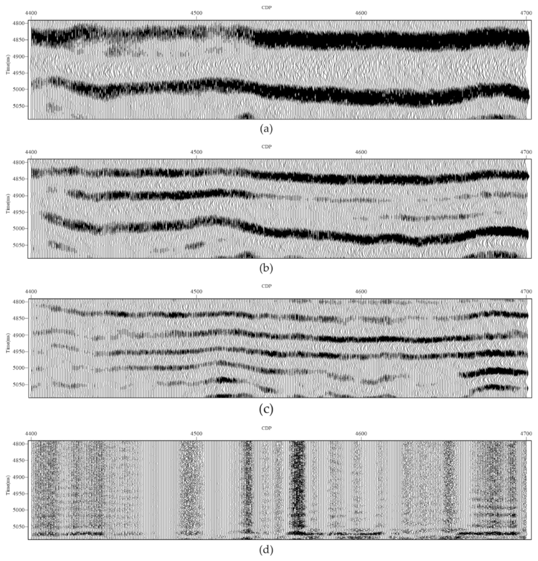
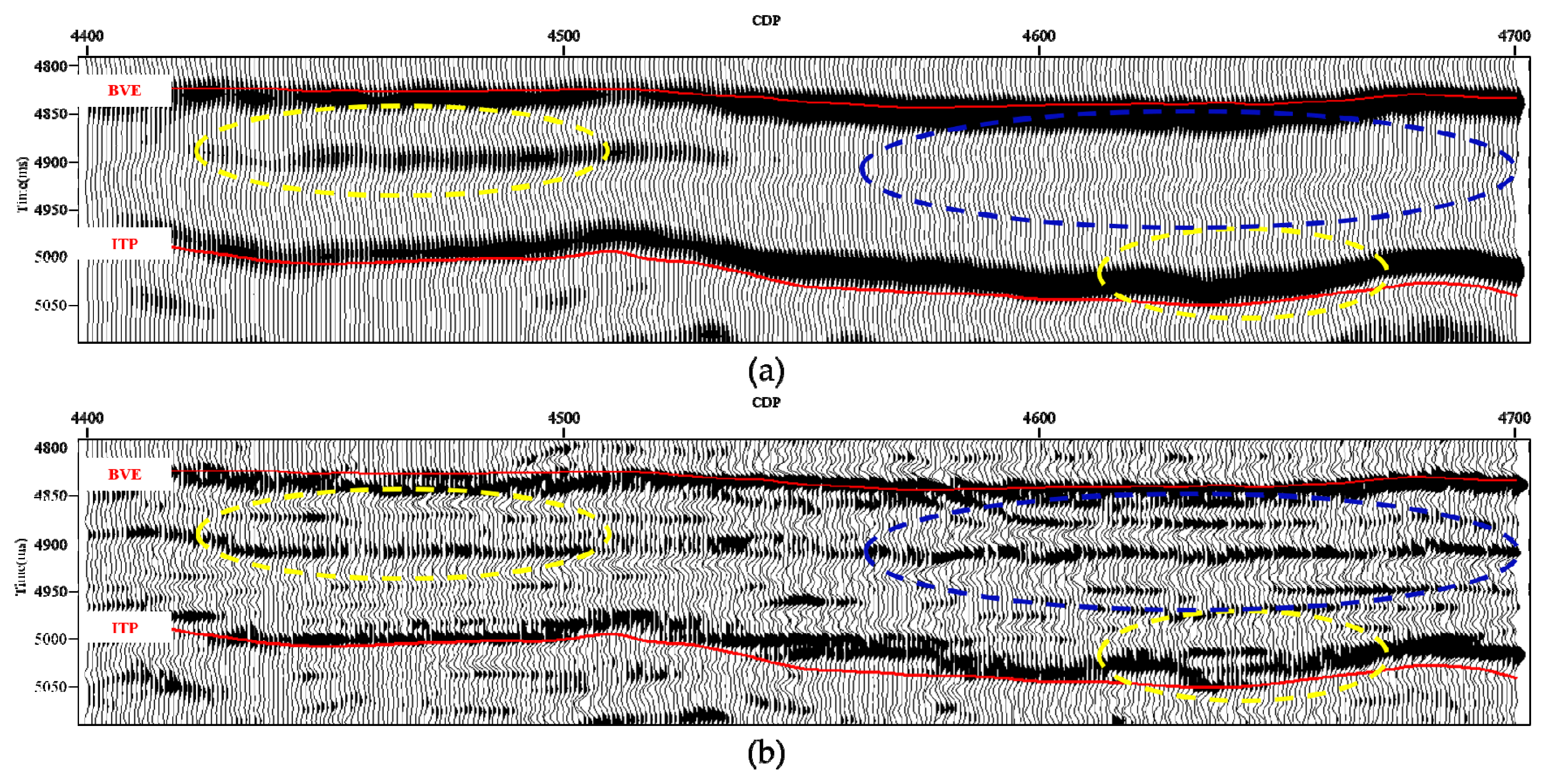
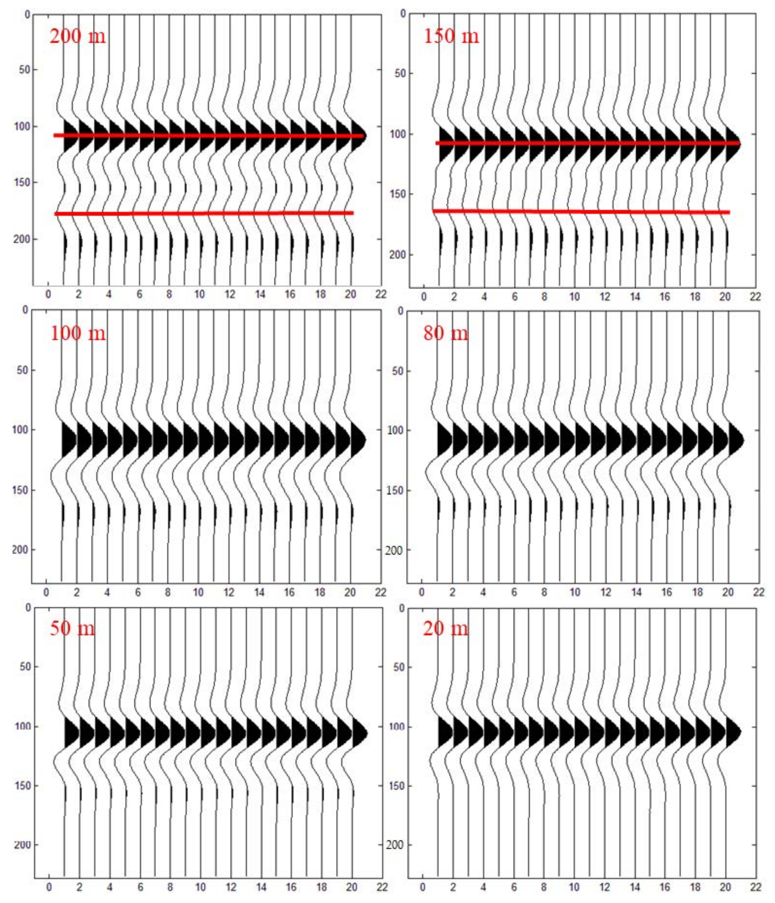
The heterogeneity of carbonate reservoirs and huge overlying rock salt make the pre-salt signal very weak. At the same time, many places show blank reflections on the seismic reflection profile, and the resolution of seismic exploration data is low. The method based on wavelet frequency decomposition processing can reasonably depict hidden details and improve the quality of pre-salt seismic signals.

2.

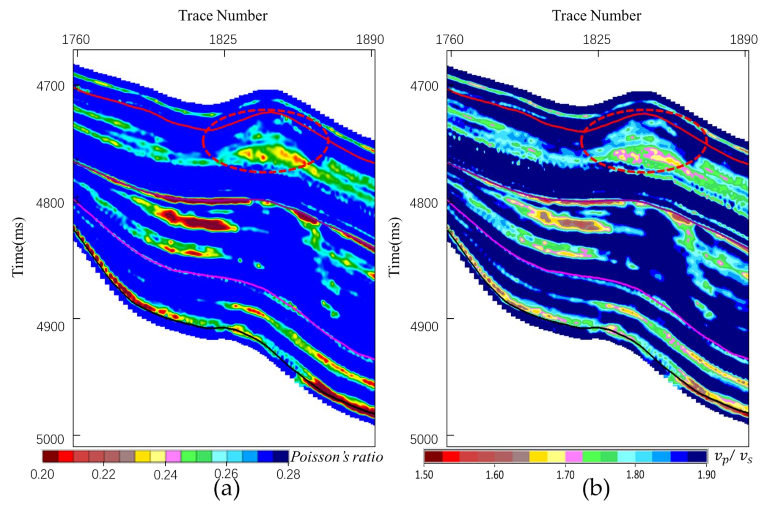
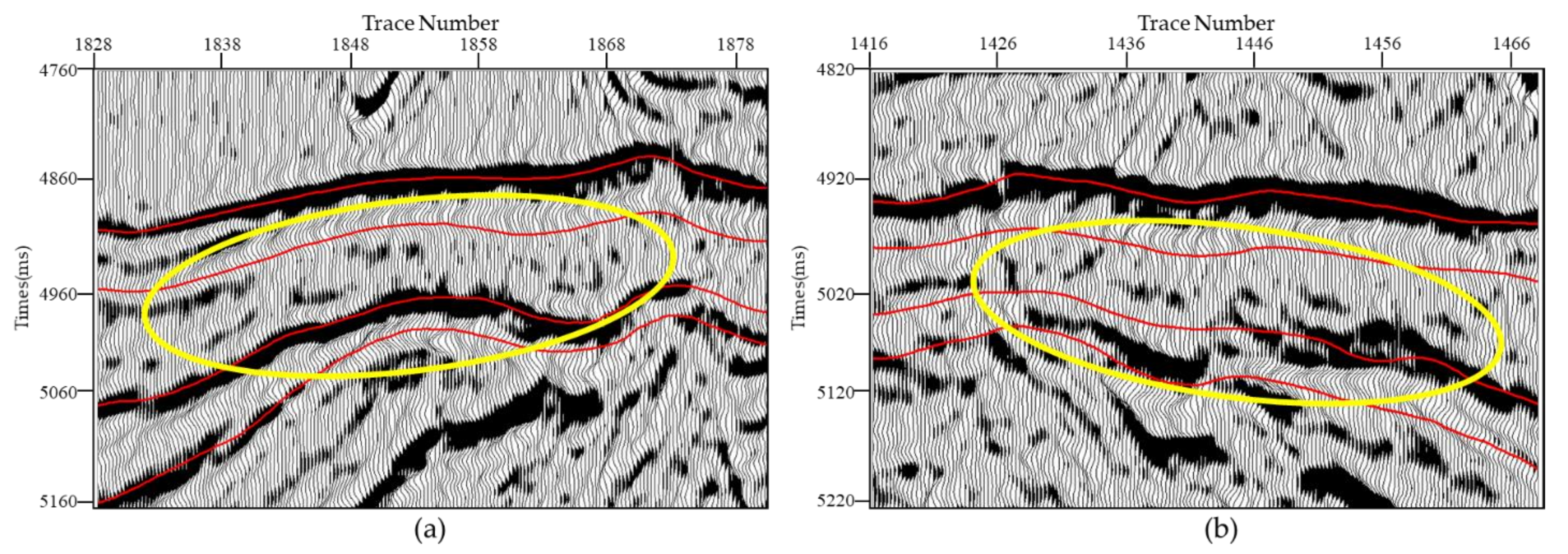
The high-precision pre-stack multiple elastic parameters simultaneous inversion method used in this paper based on Bayesian theory can obtain good reservoir inversion results and depict the growth of reefs. After that, elastic parameter inversion was performed, the Poisson’s ratio profile and $v_p/v_s$ profile can also describe the shape of the reef. To further consider whether the reef reservoir contains oil, this paper considers the study of physical parameters to characterize the oil-bearing reef as a better explanation.

3.

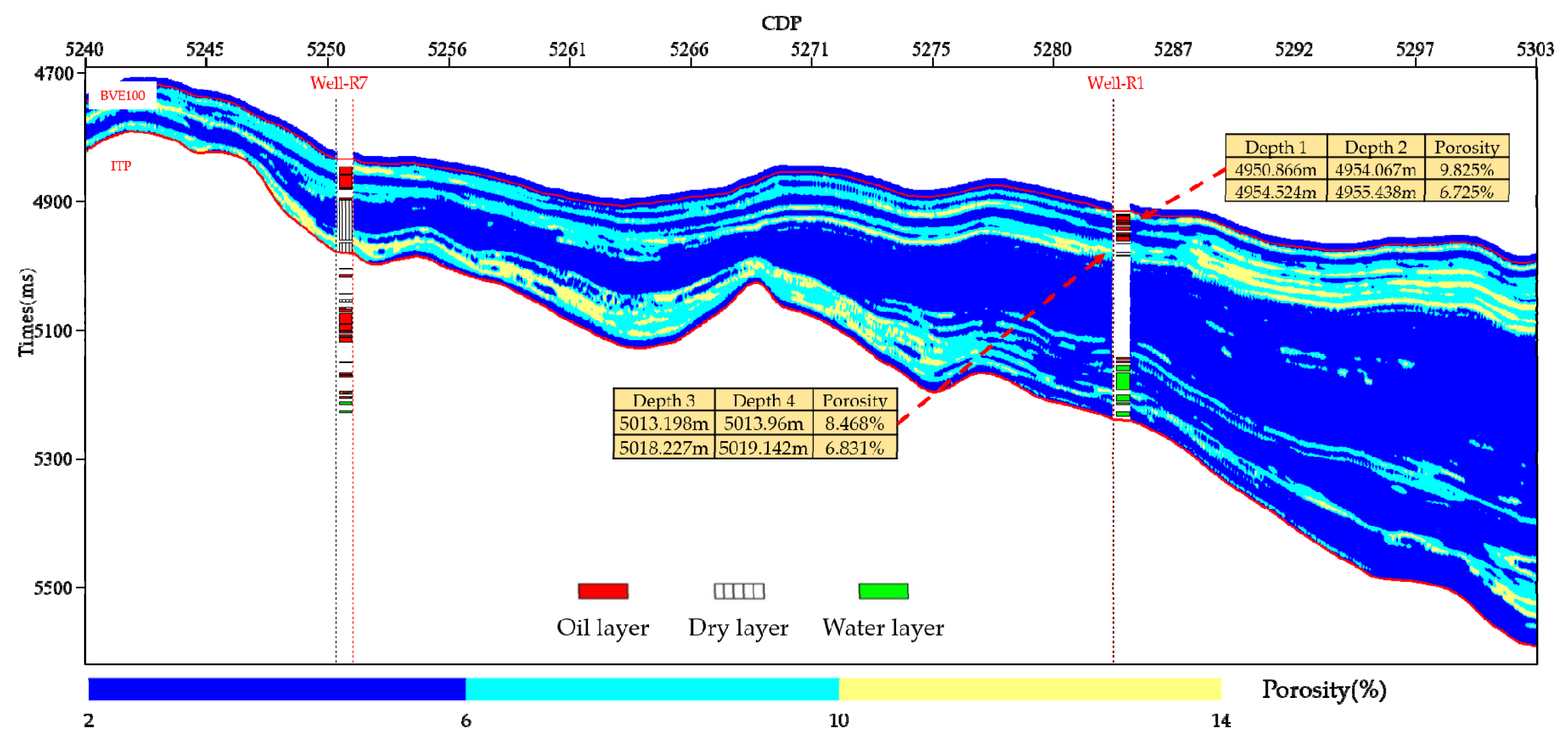
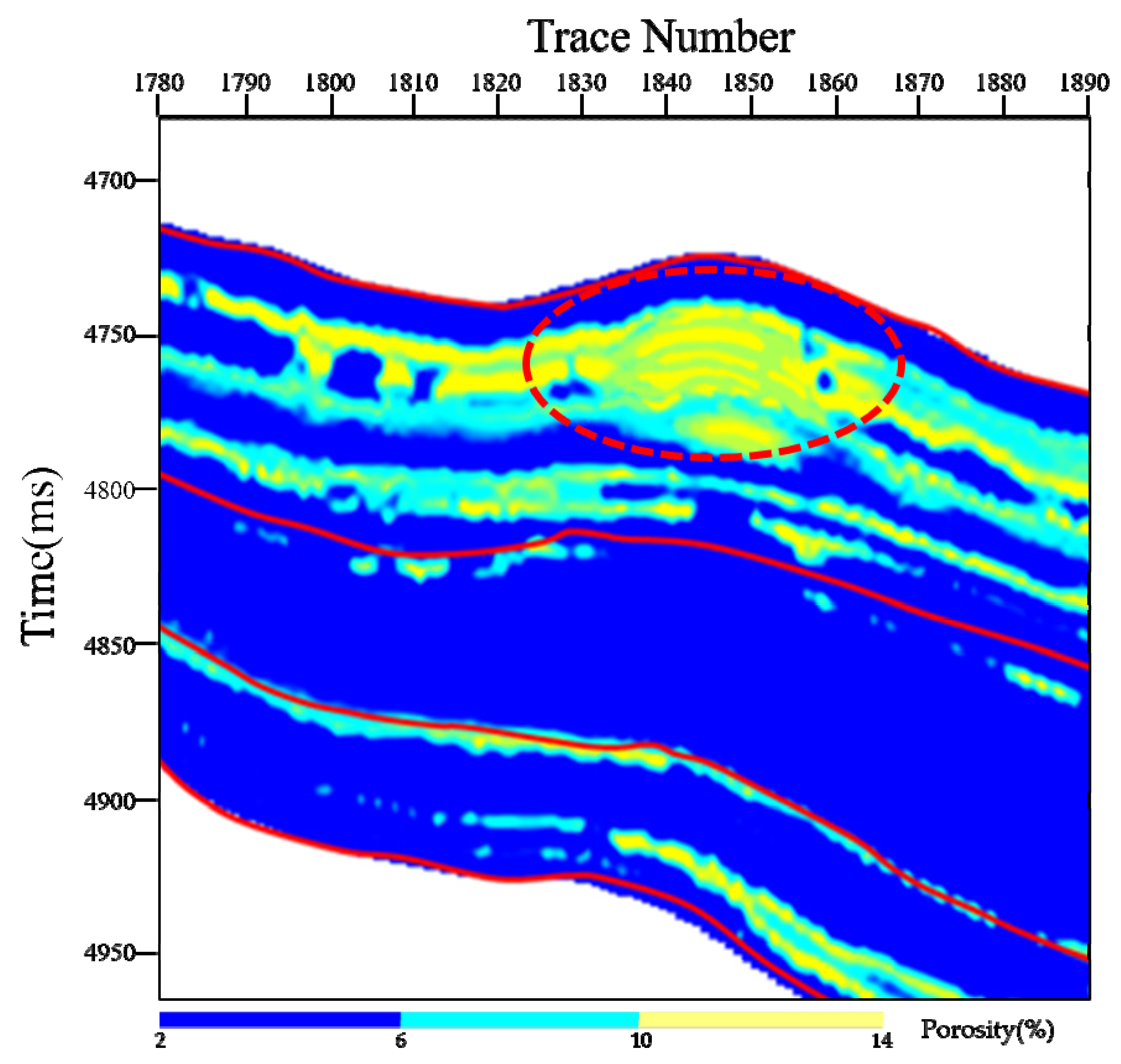
The inversion of physical property parameters based on the K-T model can obtain good porosity inversion results. Based on the high-precision pre-stack inversion in this paper, the physical property inversion method is studied. The final porosity inversion result can describe the reef more clearly than the pre-stack multiple elastic parameters inversion result and the elastic parameter inversion result, and the porosity result can better explain the oil-bearing properties of the reservoir. The inversion result is consistent with the actual drilling rock sample data and well data.

4.

This article proposed a new seismic reservoir characterization method for reference, which provides new ideas for predicting and further researching pre-salt carbonate reef reservoirs in the future.

References

1. Terra, G.J.S.; Spadini, A.R.; Franca, A.B. Carbonate rock classification applied to Brazilian sedimentary basins. Boletin De Geociencias Da Petrobras 2010, 18, 9–29. [Google Scholar]
2. Rezende, M.F.; Pope, M.C. Importance of depositional texture in pore characterization of subsalt microbialite carbonates, offshore Brazil. Geol. Soc. Lond. Spec. Publ. 2015, 418, 193–207. [Google Scholar] [CrossRef]
3. Wright, V.P.; Barnett, A.J. An abiotic model for the development of textures in some South Atlantic early Cretaceous lacustrine carbonates. Geol. Soc. Lond. Spec. Publ. 2015, 418, 209–219. [Google Scholar] [CrossRef]
4. Eberli, G.P.; Baechle, G.T.; Anselmetti, F.S.; Incze, M.L. Factors controlling elastic properties in carbonate sediments and rocks. Lead. Edge 2003, 22, 600–654. [Google Scholar] [CrossRef]
5. Roehl, P.O.; Choquette, P.W. Carbonate Petroleum Reservoirs; Springer Science and Business Media: Berlin, Germany, 2012. [Google Scholar]
6. Kerans, C. Karst-controlled reservoir heterogeneity in Ellenburger Group carbonates of west Texas. AAPG Bull. 1988, 72, 1160–1183. [Google Scholar]
7. Lucia, F.J. Rock-fabric/petrophysical classification of carbonate pore space for reservoir characterization. AAPG Bull. 1995, 79, 1275–1300. [Google Scholar]
8. Lucia, F.J.; Kerans, C.; Jennings, J.W. Carbonate reservoir characterization. J. Pet. Technol. 2003, 55, 70–72. [Google Scholar] [CrossRef]
9. Borromeo, O.; Luoni, F.; Bigoni, F.; Camocino, D.; Francesconi, A. Stratigraphic architecture of the early Carboniferous reservoir in Karachaganak field, Pri-Caspian basin (Kazakhstan). In Proceedings of the SPE Caspian Carbonates Technology Conference, Atyrau, Kazakhstan, 8–10 November 2010. [Google Scholar] [CrossRef]
10. Alsharhan, A.S.; Magara, K. Nature and distribution of porosity and permeability in Jurassic carbonate reservoirs of the Arabian Gulf Basin. Facies 1995, 32, 237–253. [Google Scholar] [CrossRef]
11. Keith, B.D. Reservoirs resulting from facies-independent dolomitization: Case histories from the Trenton and Black River carbonate rocks of the Great Lakes area. Carbonates Evaporites 1986, 1, 74–82. [Google Scholar] [CrossRef]
12. Zhao, W.Z.; Zhu, G.Y.; Zhang, S.C.; Zhao, X.F.; Sun, Y.S.; Wang, H.J.; Yang, H.J.; Han, J.F. Relationship between the later strong gas-charging and the improvement of the reservoir capacity in deep Ordovician carbonate reservoir in Tazhong area, Tarim Basin. Chin. Sci. Bull. 2009, 54, 3076–3089. [Google Scholar] [CrossRef]
13. Zou, C.N.; Xu, C.C.; Wang, Z.C.; Hu, S.Y.; Yang, G.; Li, J.; Yang, M.; Yang, Y. Geological characteristics and forming conditions of the platform margin large reef-shoal gas province in the Sichuan Basin. Pet. Explor. Dev. 2011, 38, 641–651. [Google Scholar]
14. Zhao, Z.Y.; Guo, Y.R.; Xu, W.L.; Zhang, Y.L.; Gao, J.R.; Zhang, Y.Q. Significance of three reservoir profiles for the risk exploration in Ordos Basin. Pet. Explor. Dev. 2011, 38, 16–22. [Google Scholar]
15. Ge, R.Q.; Song, C.C.; Chun, P.; Wang, R.L.; Zhang, D.W.; Xu, H.Z. Restudy on the Shahejie Formation transgression of the Paleocene in Zhan-Che sag (Jiyang depression). Geol. J. China Univ. 2003, 9, 450–457. [Google Scholar]
16. Ma, Y.Z.; Gomez, E.; Young, T.J.; Cox, D.L.; Luneau, B.; Iwere, F. Integrated reservoir modeling of a Pinedale tight-gas reservoir in the Greater Green River Basin, Wyoming. In Uncertainty Analysis and Reservoir Modeling: AAPG Memoir 96; AAPG: Tulsa, OK, USA, 2011; pp. 89–106. [Google Scholar]
17. Lima, B.E.M.; De Ros, L.F. Deposition, diagenetic and hydrothermal processes in the Aptian Pre-Salt lacustrine carbonate reservoirs of the northern Campos Basin, offshore Brazil. Sediment. Geol. 2019, 383, 55–81. [Google Scholar] [CrossRef]
18. Ryder, R.T.; Fouch, T.D.; Elson, J.H. Early Tertiary sedimentation in the western Uinta Basin. Bull. Geol. Soc. Am. 1976, 87, 496–512. [Google Scholar] [CrossRef]
19. Coogan, A.H.; Parker, M.M. Six potential trapping plays in Ordovician Trenton Limestone, Northwestern Ohio. Oil Gas J. 1984, 82, 121–126. [Google Scholar]
20. Mancini, E.A.; Llinas, J.C.; Parcell, W.C.; Aurell, M.; Badenas, B.; Leinfelder, R.R.; Benson, D.J. Upper Jurassic thrombolite reservoir play, northeastern Gulf of Mexico. AAPG Bull. 2004, 88, 1573–1602. [Google Scholar] [CrossRef]
21. Van Tuyl, J.; Alves, T.M.; Cherns, L. Geometric and depositional responses of carbonate build-ups to Miocene sea level and regional tectonics offshore northwest Australia. Mar. Pet. Geol. 2018, 94, 144–165. [Google Scholar] [CrossRef]
22. Zhao, W.Z.; Shen, A.J.; Hu, S.Y.; Zhang, B.M.; Pan, W.Q.; Zhou, J.G.; Wang, Z.C. Geological conditions and distributional features of large-scale carbonate reservoirs onshore China. Pet. Explor. Dev. 2012, 39, 1–14. [Google Scholar] [CrossRef]
23. Tavakoli, V. Carbonate Reservoir Heterogeneity: Overcoming the Challenges; Springer Nature: Basingstoke, UK, 2019. [Google Scholar]
24. Riding, R. Microbial carbonates: The geological record of calcified bacterial–algal mats and biofilms. Sedimentology 2000, 47, 179–214. [Google Scholar] [CrossRef]
25. Ahr, W.M. Geology of Carbonate Reservoirs: The Identification, Description and Characterization of Hydrocarbon Reservoirs in Carbonate Rocks; John Wiley and Sons: Hoboken, NJ, USA, 2011. [Google Scholar]
26. Moore, C.H.; Wade, W.J. Carbonate Reservoirs: Porosity and Diagenesis in a Sequence Stratigraphic Framework; Elsevier: Amsterdam, The Netherlands, 2013. [Google Scholar]
27. Mohriak, W.U.; Perdomo, L.V.; Plucenio, D.M.; Saad, J. Challenges for petrophysical characterization of presalt carbonate reservoirs. In Proceedings of the 14th International Congress of the Brazilian Geophysical Society EXPOGEF, Rio de Janeiro, Brazil, 3–6 August 2015; pp. 623–627. [Google Scholar]
28. Saller, A.; Rushton, S.; Buambua, L.; Inman, K.; McNeil, R.; Dickson, J.A.D. Presalt stratigraphy and depositional systems in the Kwanza Basin, offshore Angola. AAPG Bull. 2016, 100, 1135–1164. [Google Scholar] [CrossRef]
29. Ronchi, P.; Ortenzi, A.; Borromeo, O.; Claps, M.; Zempolich, W. Depositional setting and diagenetic processes and their impact on the reservoir quality in the late Visean–Bashkirian Kashagan carbonate platform (Pre-Caspian Basin, Kazakhstan). AAPG Bull. 2010, 94, 1313–1348. [Google Scholar] [CrossRef]
30. Kenter, J.A.M.; Harris, P.M.; Collins, J.F. The Microbial-Dominated Slopes of Tengiz Field, Pricaspian Basin, Kazakhstan. In Proceedings of the Core Workshop: American Association of Petroleum Geologists Hedberg Conference on Microbial Carbonate Reservoir Characterization, Houston, TX, USA, 4–8 June 2012; p. 4. [Google Scholar]
31. Collins, J.F.; Katz, D.; Harris, P.M.; Narr, W. Burial Cementation and Dissolution in Carboniferous Slope Facies, Tengiz Field, Kazakhstan: Evidence for Hydrothermal Activity. In Proceedings of the AAPG Search and Discovery Article, London, UK, 27 January 2014; Volume 20234. [Google Scholar]
32. Searle, A.; Xing, H.; Iskakov, E.; Jazbayev, K.; Jenkins, S.D.; Lee, K.S.; McLean, N. A Comprehensive Anisotropic Velocity Model Building Case Study—Tengiz Full Azimuth Land TTI PSDM. In Proceedings of the 76th EAGE Conference and Exhibition, Amsterdam, The Netherlands, 16–19 June 2014. [Google Scholar]
33. Cheng, T.; Kang, H.Q.; Bai, B. Key technologies and their application in exploration of pre-salt lacustrine carbonate rock in Santos basin, Brazil. China Offshore Oil Gas 2018, 30, 27–35. [Google Scholar]
34. Gomes, J.P.; Bunevich, R.B.; Tedeschi, L.R.; Tucker, M.E.; Whitaker, F.F. Facies classification and patterns of lacustrine carbonate deposition of the Barra Velha Formation, Santos Basin, Brazilian Pre-salt. Mar. Pet. Geol. 2020, 113, 104–176. [Google Scholar] [CrossRef]
35. De Paula Faria, D.L.; dos Reis, A.T.; de Souza, O.G., Jr. Three-dimensional stratigraphic-sedimentological forward modeling of an Aptian carbonate reservoir deposited during the sag stage in the Santos basin, Brazil. Mar. Pet. Geol. 2017, 88, 676–695. [Google Scholar] [CrossRef]
36. Yang, X.L. Comparison of subsalt hydrocarbon accumulation characteristics in basins on both sides of the Mid-South Atlantic. Offshore Oil. 2019, 3, 1–8. [Google Scholar]
37. Wu, J.; Zhao, P.F.; Wang, H.; Wang, Y.Q.; Li, J.G. Paleogeomorphology of the barra velha formation in block a of the Santos Basin, Brazil, and its control over reservoirs. Mar. Geol. Front. 2019, 35, 56–62. [Google Scholar]
38. Alves, T.M.; Fetter, M.; Lima, C.; Cartwright, J.A.; Cosgrove, J.; Ganga, A.; Queiroz, C.L.; Strugale, M. An incomplete correlation between pre-salt topography, top reservoir erosion, and salt deformation in deep-water Santos Basin. Mar. Pet. Geol. 2017, 79, 300–320. [Google Scholar] [CrossRef]
39. Kuster, G.T.; Toksoz, M.N. Velocity and attenuation of seismic waves in two-phase media: Part, I. Theoretical formulations. Geophysics 1974, 39, 587–606. [Google Scholar] [CrossRef]
40. Mavko, G.; Mukerji, T.; Dvorkin, J. The Rock Physics Handbook: Tools for Seismic Analysis of Porous Media; Cambridge University Press: Cambridge, UK, 1998. [Google Scholar]
41. Williams, B.G.; Hubbard, R.J. Seismic stratigraphic framework and depositional sequences in the Santos Basin, Brazil. Mar. Pet. Geol. 1984, 1, 90–104. [Google Scholar] [CrossRef]
42. Ojeda, H. Structural framework, stratigraphy and evolution of Brazilian marginal basins. AAPG Bull. 1982, 66, 732–749. [Google Scholar]
43. Cainelli, C.; Mohriak, W.U. Geology of Atlantic eastern Brazilian basins. Braz. Geol. Part 1998, 2, 1998. [Google Scholar]
44. Szatmari, P.; Milani, E.; Lana, M.; Conceicao, J.; Lobo, A. How South Atlantic rifting affects Brazilian oil reserves. Oil Gas J. 1985, 83, 107–113. [Google Scholar]
45. Cainelli, C.; Mohriak, W.U. Some remarks on the evolution of sedimentary basins along the Eastern Brazilian continental margin. Epis.-Newsmag. Int. Union Geol. Sci. 1999, 22, 206–216. [Google Scholar] [CrossRef] [Green Version]
46. Stanton, N.; Ponte-Neto, C.; Bijani, R.; Masini, E.; Fontes, S.; Flexor, J.M. A geophysical view of the Southeastern Brazilian margin at Santos Basin: Insights into rifting evolution. J. S. Am. Earth Sci. 2014, 55, 141–154. [Google Scholar] [CrossRef]
47. Castagna, J.P.; Sun, S. Comparison of spectral decomposition methods. First Break 2006, 24. [Google Scholar] [CrossRef]
48. Weinstein, S.; Ebert, P. Data transmission by frequency-division multiplexing using the discrete Fourier transform. IEEE Trans. Commun. Technol. 1971, 19, 628–634. [Google Scholar] [CrossRef]
49. Griffin, D.; Lim, J. Signal estimation from modified short-time Fourier transform. IEEE Trans. Acoust. Speech Signal Process. 1984, 32, 236–243. [Google Scholar] [CrossRef]
50. Zhang, R.; Fomel, S. Time-variant wavelet extraction with a local-attribute-based time-frequency decomposition for seismic inversion. Interpretation 2017, 5, 9–16. [Google Scholar] [CrossRef]
51. Sinha, S.; Routh, P.S.; Anno, P.D.; Castagna, J.P. Spectral decomposition of seismic data with continuous-wavelet transform. Geophysics 2005, 70, 19–25. [Google Scholar] [CrossRef]
52. Huang, H.D.; Zhang, R.W.; Guo, Y.C. Wavelet frequency-division process for seismic signals. J. Oil Gas Technol. 2008, 30, 87–91. [Google Scholar]
53. Rhif, M.; Ben Abbes, A.; Farah, I.R.; Martínez, B.; Sang, Y. Wavelet transform application for/in non-stationary time-series analysis: A review. Appl. Sci. 2019, 9, 1345. [Google Scholar] [CrossRef] [Green Version]
54. Portniaguine, O.; Castagna, J. Inverse spectral decomposition. SEG Tech. Program Expand. Abstr. 2004, 2004, 1786–1789. [Google Scholar]
55. Vetterli, M.; Herley, C. Wavelets and filter banks: Theory and design. IEEE Trans. Signal Process. 1992, 40, 2207–2232. [Google Scholar] [CrossRef] [Green Version]
56. Resnikoff, H.L.; Raymond, O., Jr. Wavelet Analysis: The Scalable Structure of Information; Springer Science and Business Media: Berlin, Germany, 2012. [Google Scholar]
57. Shensa, M.J. The discrete wavelet transform: Wedding the a trous and Mallat algorithms. IEEE Trans. Signal Process. 1992, 40, 2464–2482. [Google Scholar] [CrossRef] [Green Version]
58. Tian, X.D.; Huang, H.D.; Luo, Y.N. Deepwater sub-salt carbonate reef reservoir prediction in Santos Basin, Brazil. SEG Tech. Program Expand. Abstr. 2019, 2019, 534–538. [Google Scholar]
59. Huang, H.D.; Yuan, S.Y.; Zhang, Y.T.; Zeng, J.; Mu, W.T. Use of nonlinear chaos inversion in predicting deep thin lithologic hydrocarbon reservoirs: A case study from the Tazhong oil field of the Tarim Basin, China. Geophysics 2016, 81, B221–B234. [Google Scholar] [CrossRef]
60. Liu, Z.S.; Sun, Z.D.; Dong, N.; Liu, J.Z.; Liu, Z.X.; Wang, Y.J. A modified Kuster-Toksöz rock physics model and its application. Oil Geophys. Prospect. 2018, 53, 113–121. [Google Scholar]
61. Gassmann, F. Elastic waves through a packing of spheres. Geophysics 1951, 16, 673–685. [Google Scholar] [CrossRef]
Figure 1. A typical common depth point (CDP) seismic profile of a survey line in the work area. The red arrow area shows that the salt layer causes the signal to be significantly absorbed. The blue arrow area indicates that the signal-to-noise ratio of the pre-salt carbonate reservoir is low, and the seismic events are intermittent.
Minerals 11 00973 g001
Figure 2. The seismic profile results were obtained by decomposing the wavelet into four different narrow bands from low frequency to high frequency. The frequency range is (a) 0–10 Hz; (b) 10–20 Hz; (c) 20–30 Hz; (d) 30–40 Hz. Since the primary frequency of seismic data is low, the high-frequency result in the last panel is mainly noise.
Minerals 11 00973 g002
Figure 3. Comparison of images before and after wavelet frequency decomposition processing. (a) The panel above is the result of not using wavelet frequency decomposition processing; (b) the panel below shows the result of the wavelet decomposition process. Multiple seismic events and evident complex waves obtained in the yellow circles and the blue circle area originally displayed as blank now depicts three seismic events.
Minerals 11 00973 g003
Figure 4. (a) Original seismic data. The multiple elastic parameters pre-stack seismic inversion results of: (b) P-wave velocity; (c) S-wave velocity; (d) density. These ellipticals indicate carbonate reservoirs with the characteristics of reefs.
Minerals 11 00973 g004
Figure 5. (a) Poisson’s ratio inversion profile; (b) v p / v s inversion profile. The ellipses indicate carbonate reservoirs with reef characteristics.
Minerals 11 00973 g005
Figure 6. The porosity inversion profile and the correspondence between the inversion results and well-logging information.
Minerals 11 00973 g006
Figure 7. Comparison analysis graph of porosity obtained by inversion, rock samples porosity, and well-logging porosity.
Minerals 11 00973 g007
Figure 8. Porosity inversion results based on high-precision pre-stack inversion. The red circle can more clearly describe the layered stack of reef reservoirs and help to quantitatively indicate the potential favorable oil-gas possibility area.
Minerals 11 00973 g008
Figure 9. Examples of four different reef seismic reflection responses in the work area. The yellow ellipses mark (a) mound-like reflections, moderate internal reflections, and a hanging structure; (b) strong reflection at the top, no internal reflection, and an asymmetrical structure; (c) waveform protrudes, part of the phase axis is interrupted and the bottom energy is weak; (d) moderately strong reflection, the event axis is inclined at the bottom interface and the top reflection.
Minerals 11 00973 g009
Figure 10. Examples of two different reef-shoal seismic reflection responses in the work area. The yellow ellipses mark (a) chaotic internal reflections and weak reflections; and (b) weak amplitude and blank reflections.
Minerals 11 00973 g010
Figure 11. Wave characteristics of the BVE group in the work area.
Minerals 11 00973 g011
Figure 12. Forward simulation of different gypsum thicknesses.
Minerals 11 00973 g012
Publisher’s Note: MDPI stays neutral with regard to jurisdictional claims in published maps and institutional affiliations.