
Simulation Technology Development for Dynamic Analysis of Mechanical System in Deep-Seabed Integrated Mining System Using Multibody Dynamics


Abstract
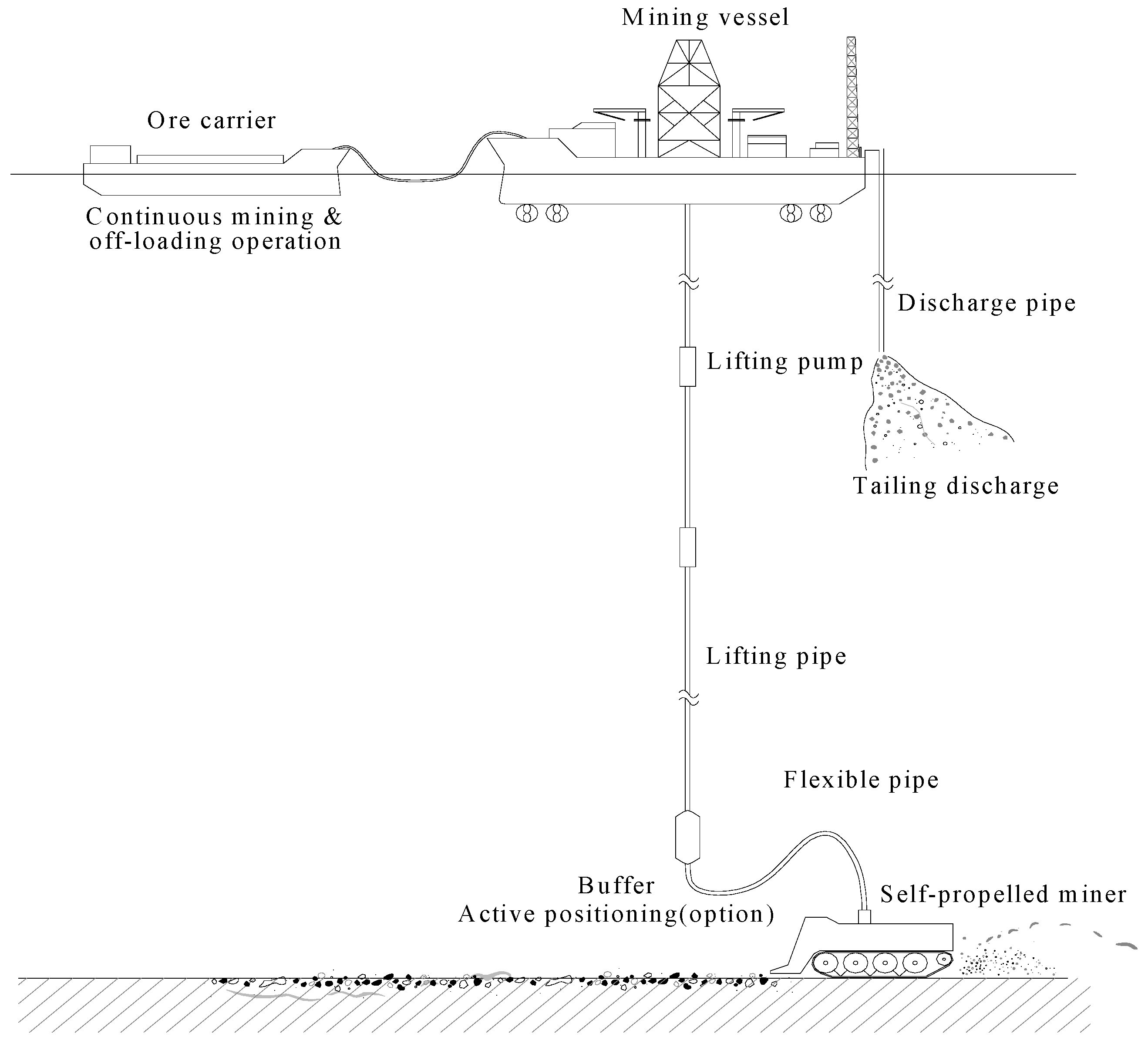
:1. Introduction
2. Multibody Dynamics
3. Development of Environmental Modeling Technologies
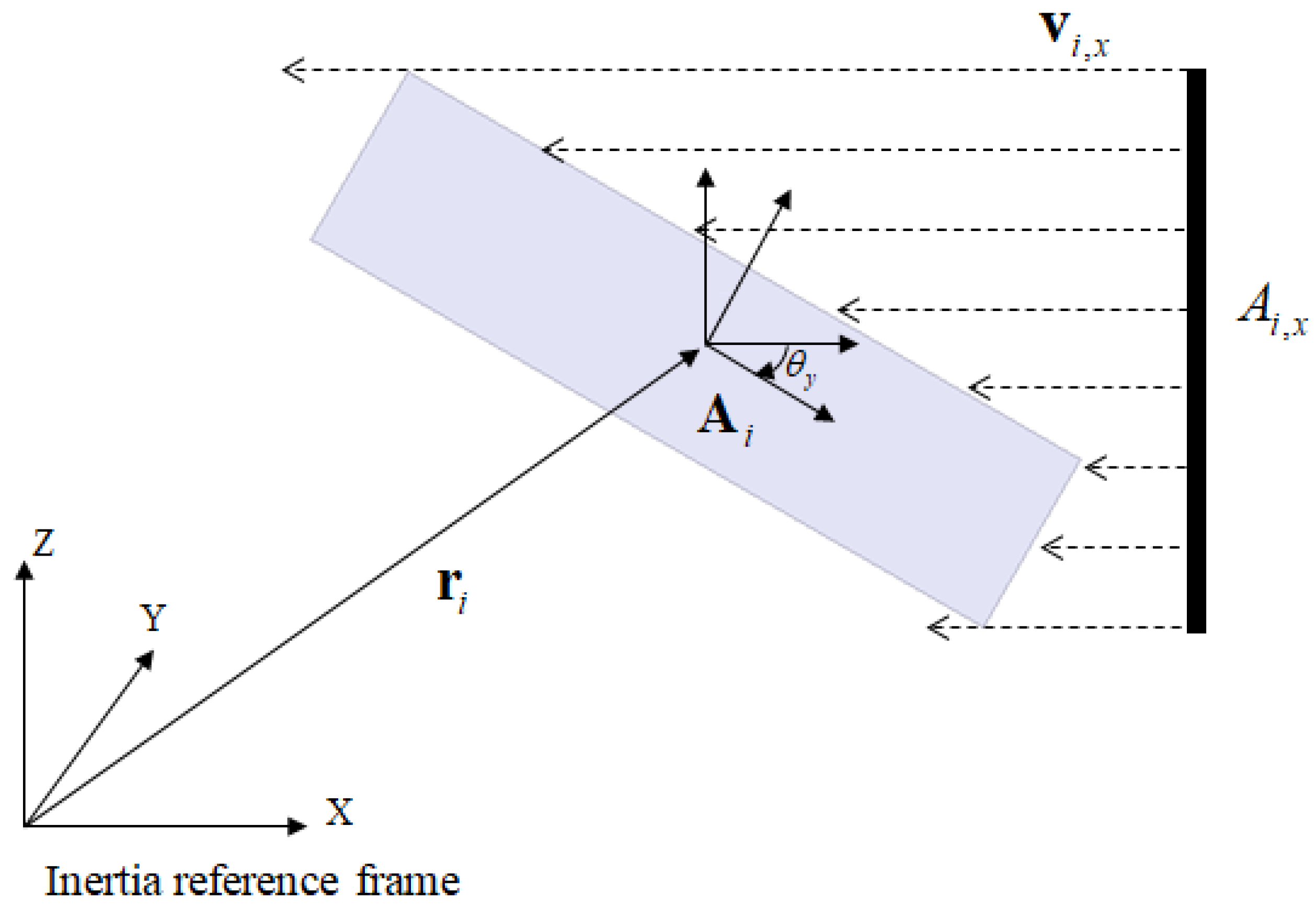
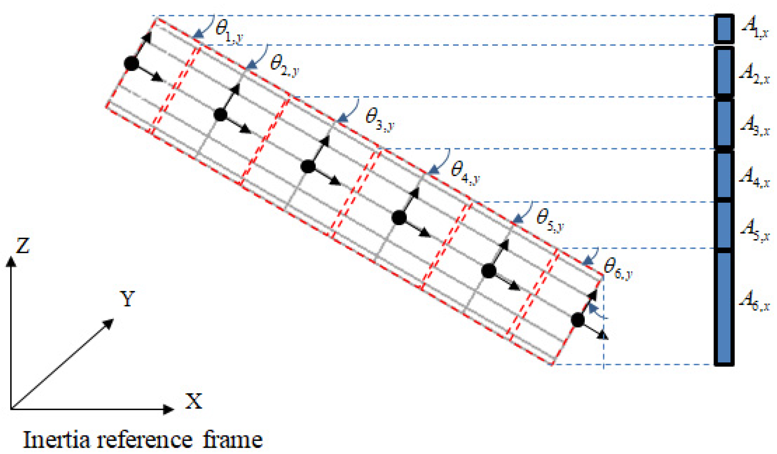
3.1. Formulations of Hydrodynamics
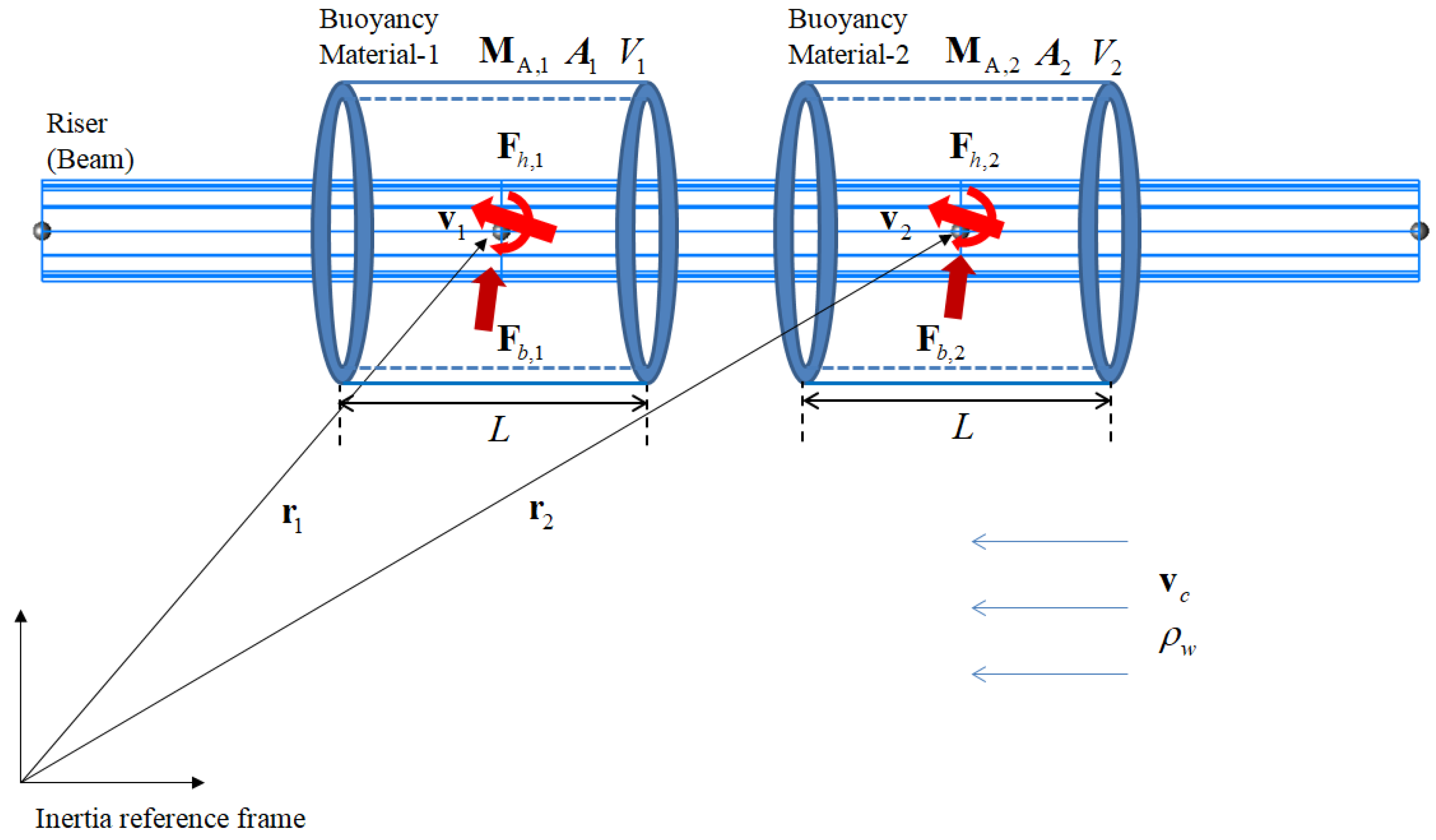
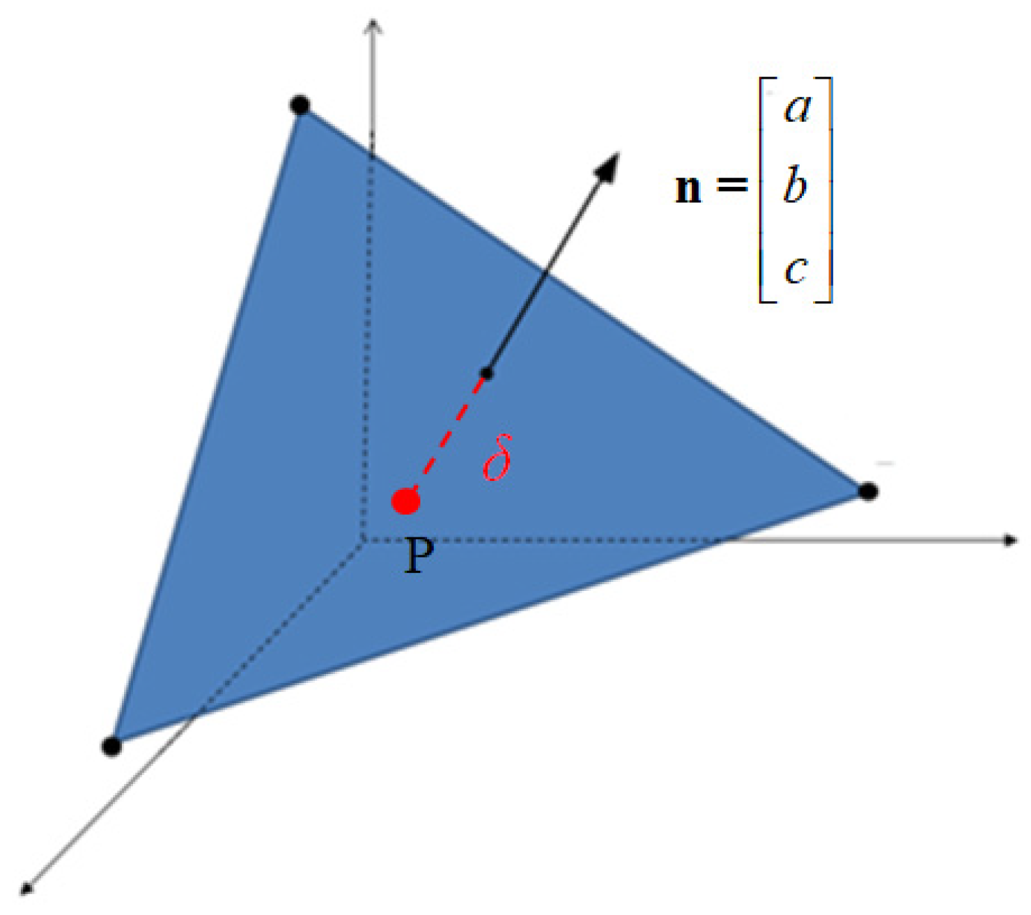
3.2. Formulation of Buoyancy Force
3.3. Formulations of Ocean Current
4. Development of Mechanical System Modeling Technologies
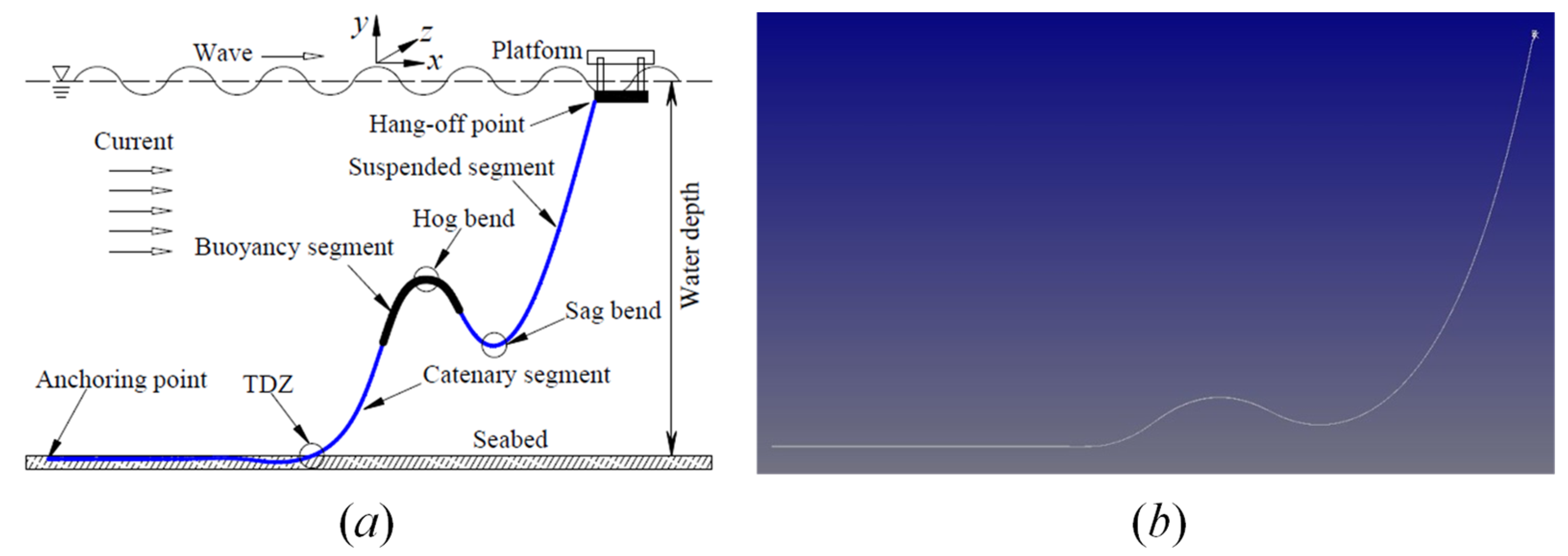
4.1. Riser System
Formulations of Beam Elastic Theory
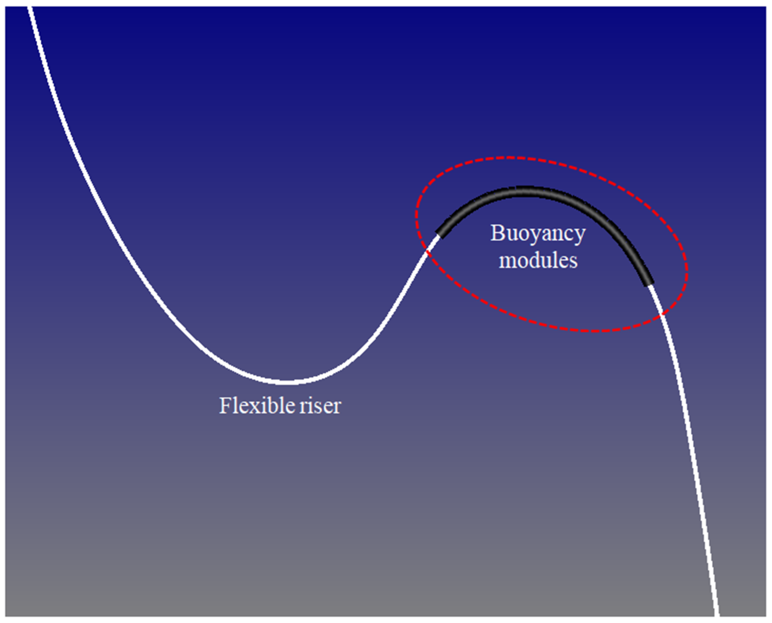
4.2. Formulations of Buoyancy Modules
4.3. Formulations of Mining Vessel
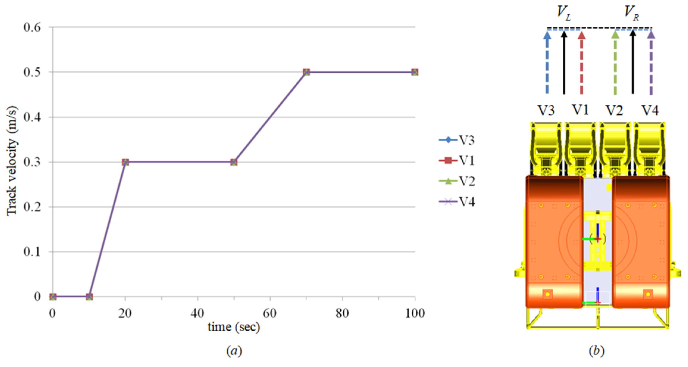
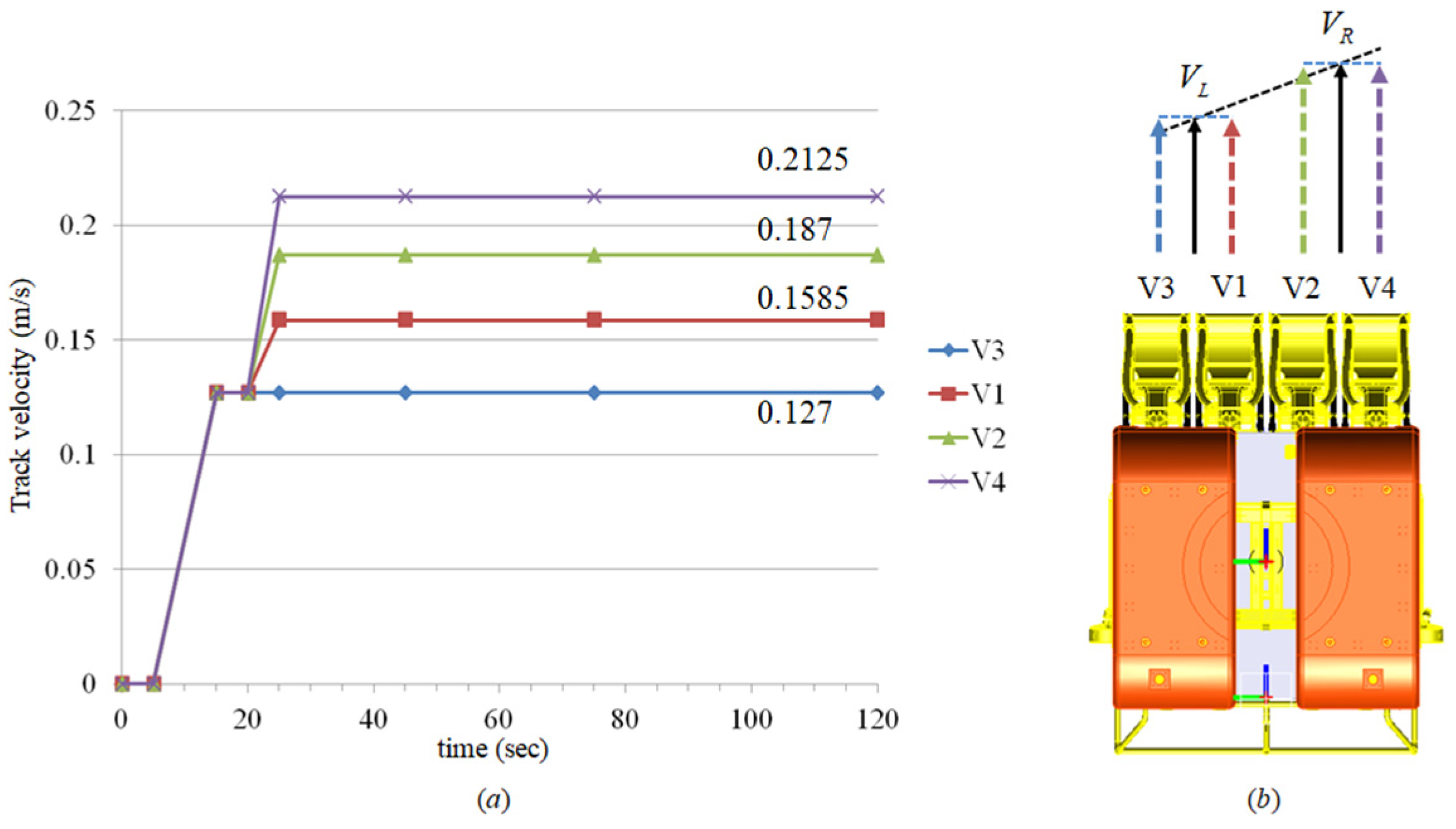
4.4. Formulations of Mining Robot
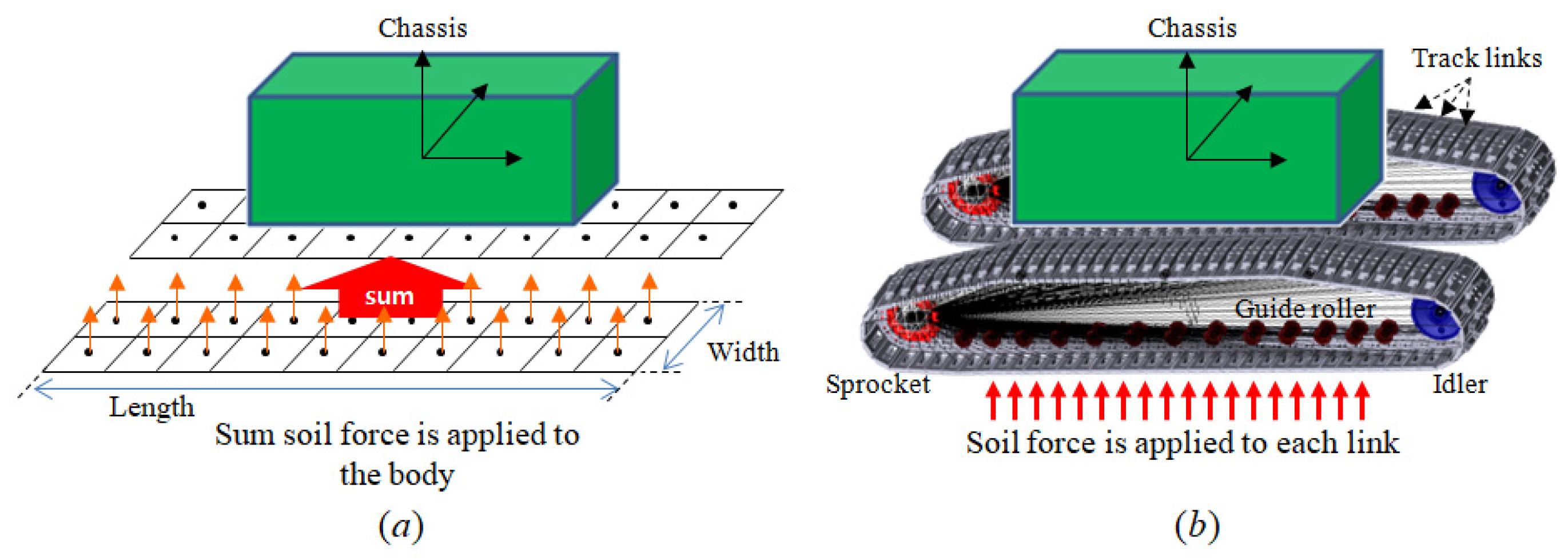
4.4.1. Formulations of Single-Body Track Model for Mining Robot
4.4.2. Formulations of Multibody Track Model for Mining Robot
5. Development of Soil Contact Mechanism
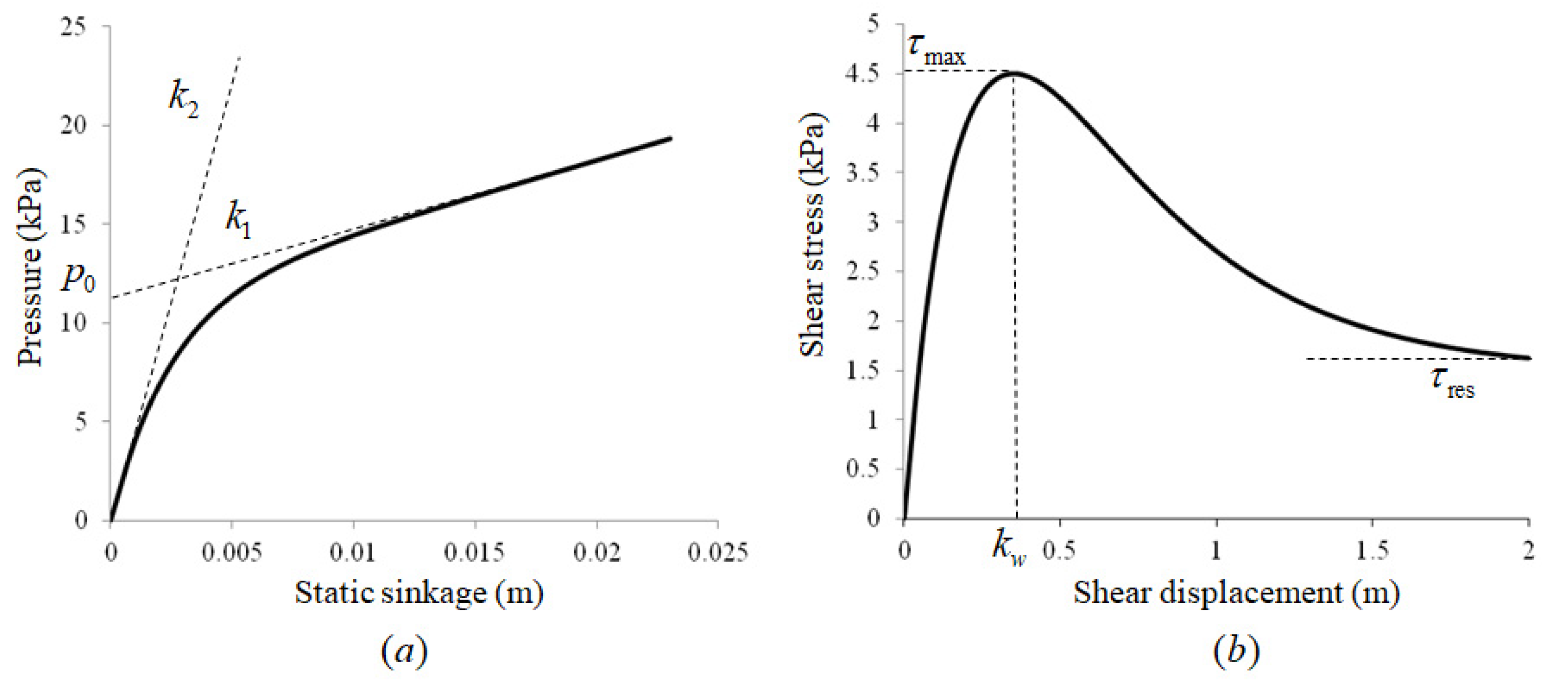
5.1. Formulations of Soil Contact Force
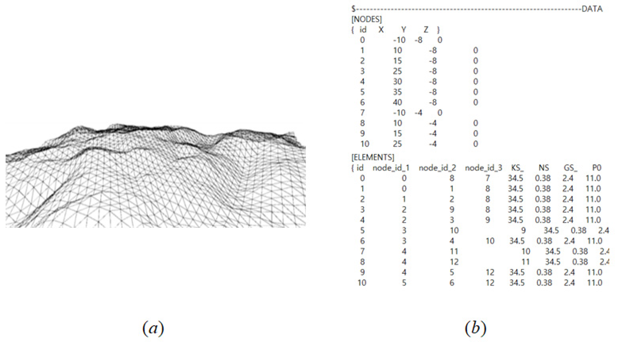
5.2. Formulations for Three-Dimensional Ground
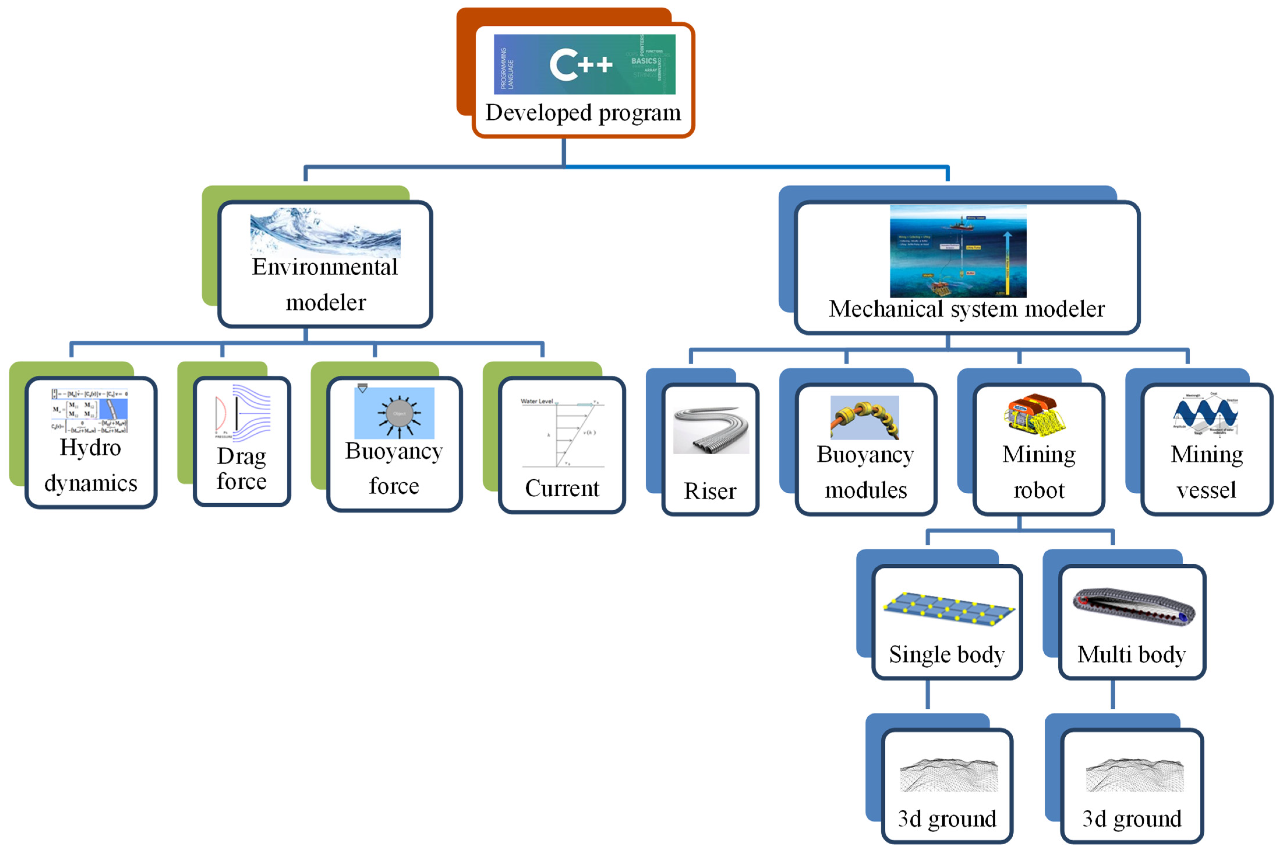
6. Structure and User Interface of Modelers
6.1. User Interface of Environmental Modelers
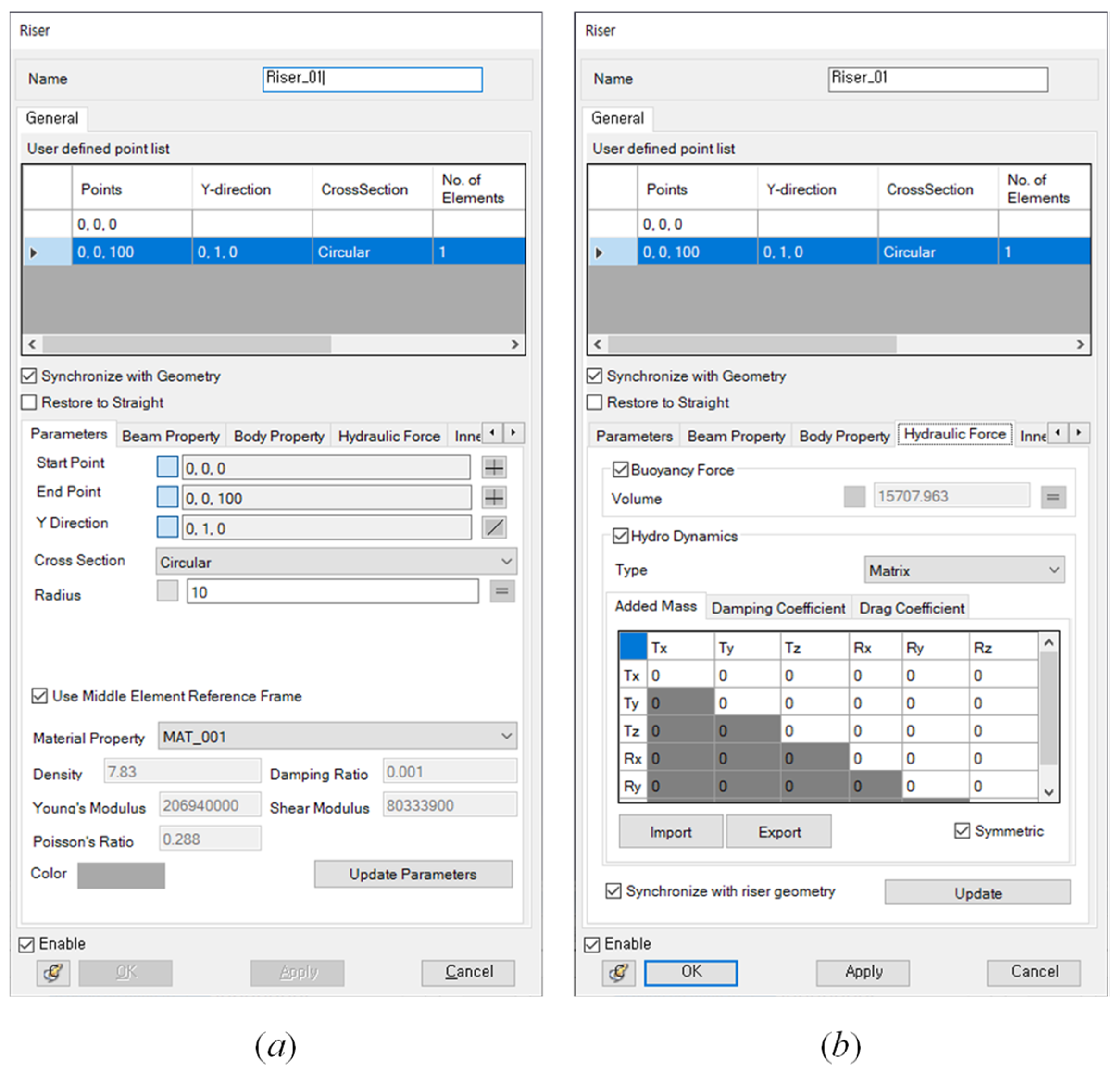
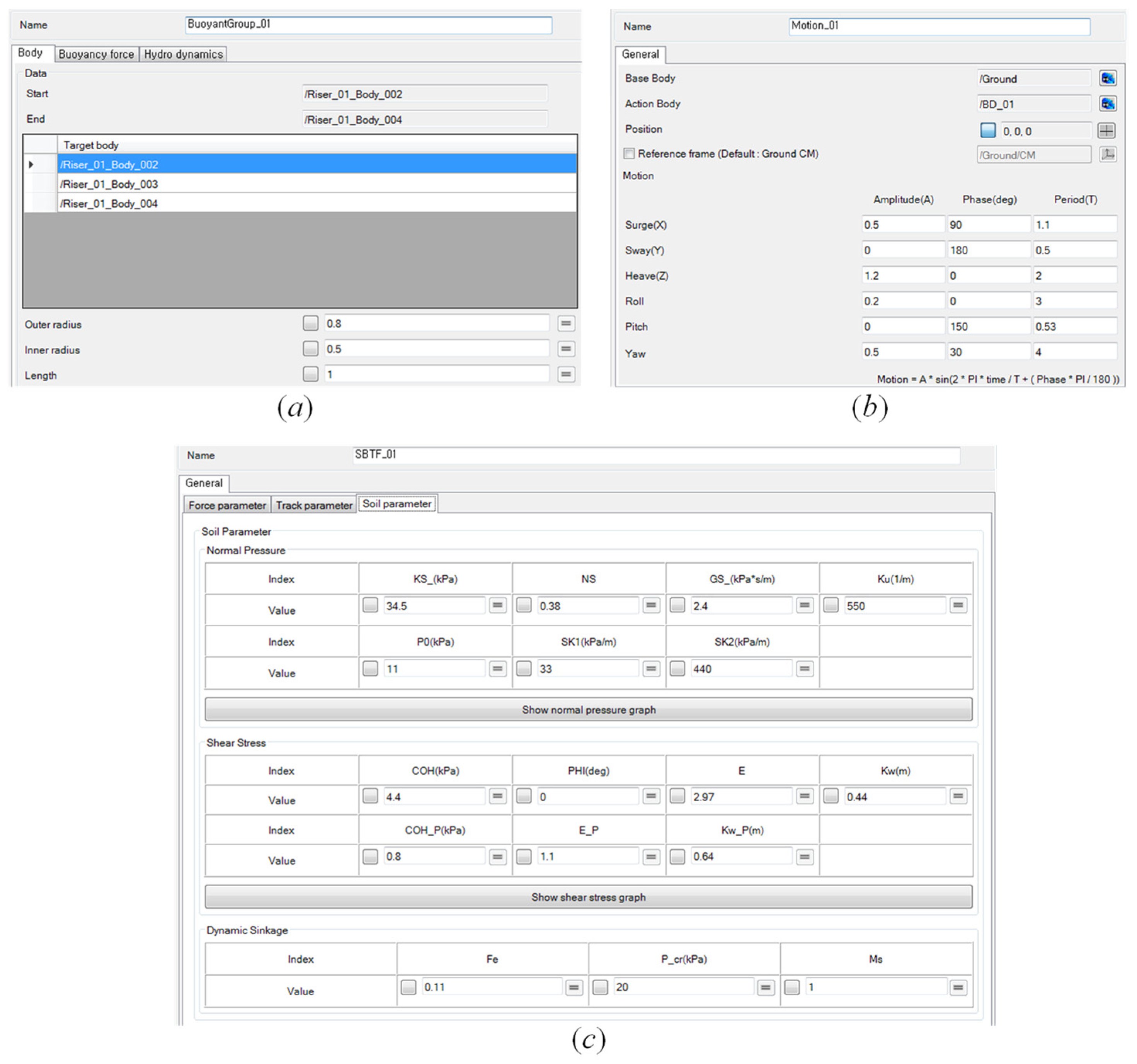
6.2. User Interface of Mechanical System Modelers
7. Verification
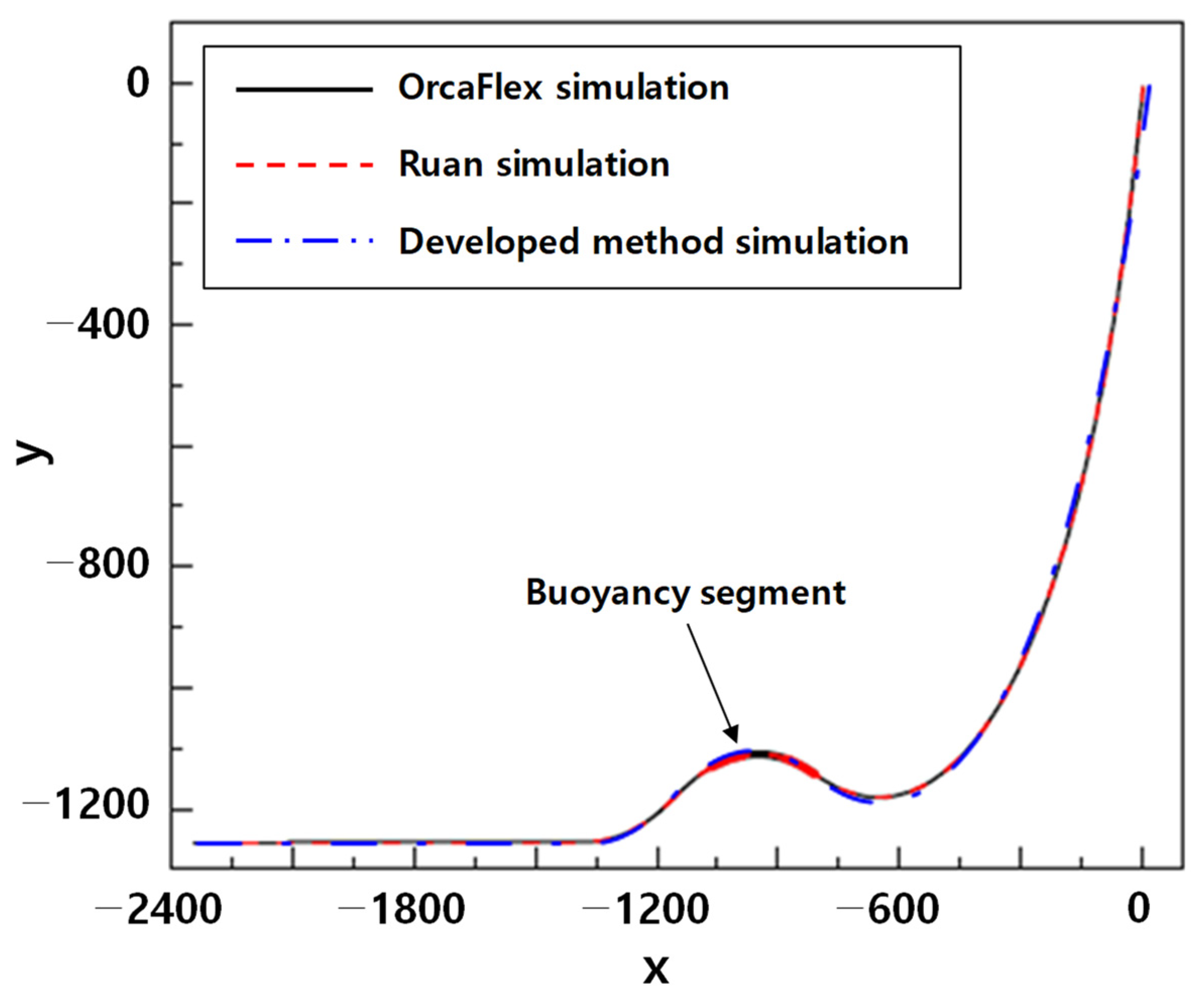
7.1. Offshore Riser System
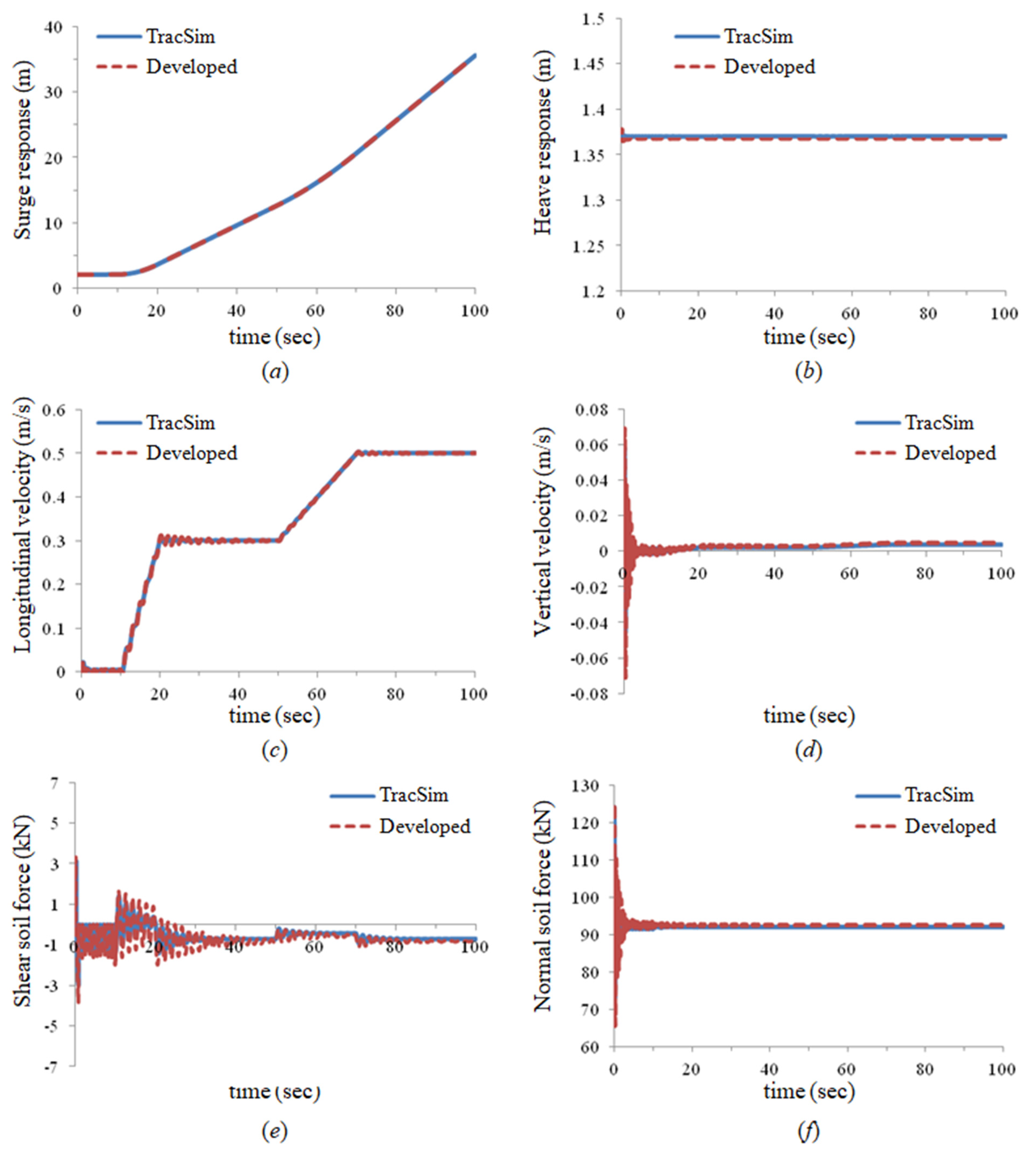
7.2. Soil Contact Mechanism
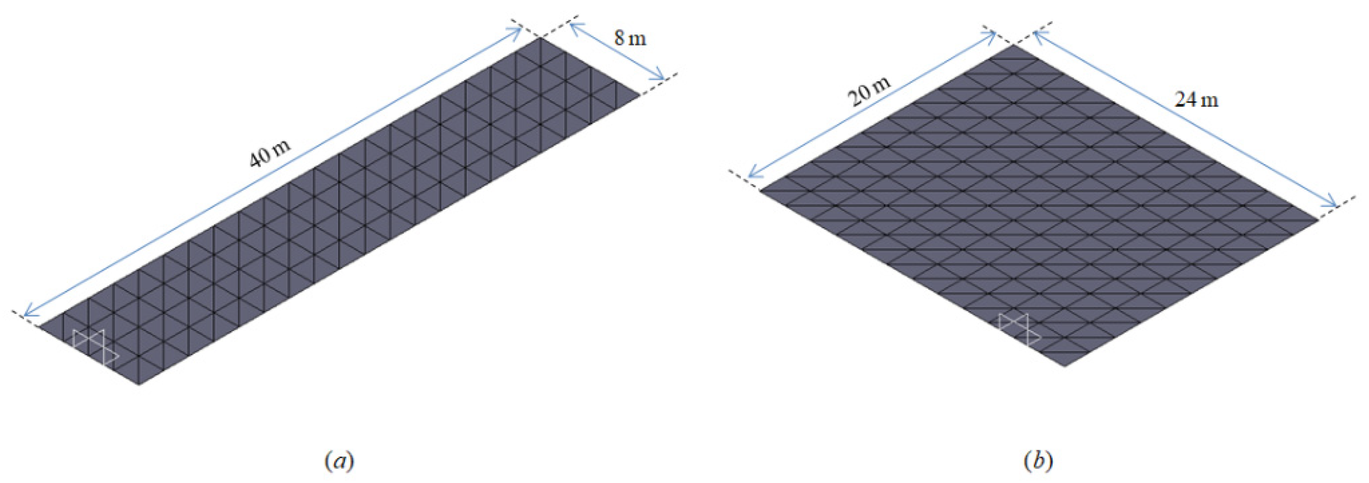
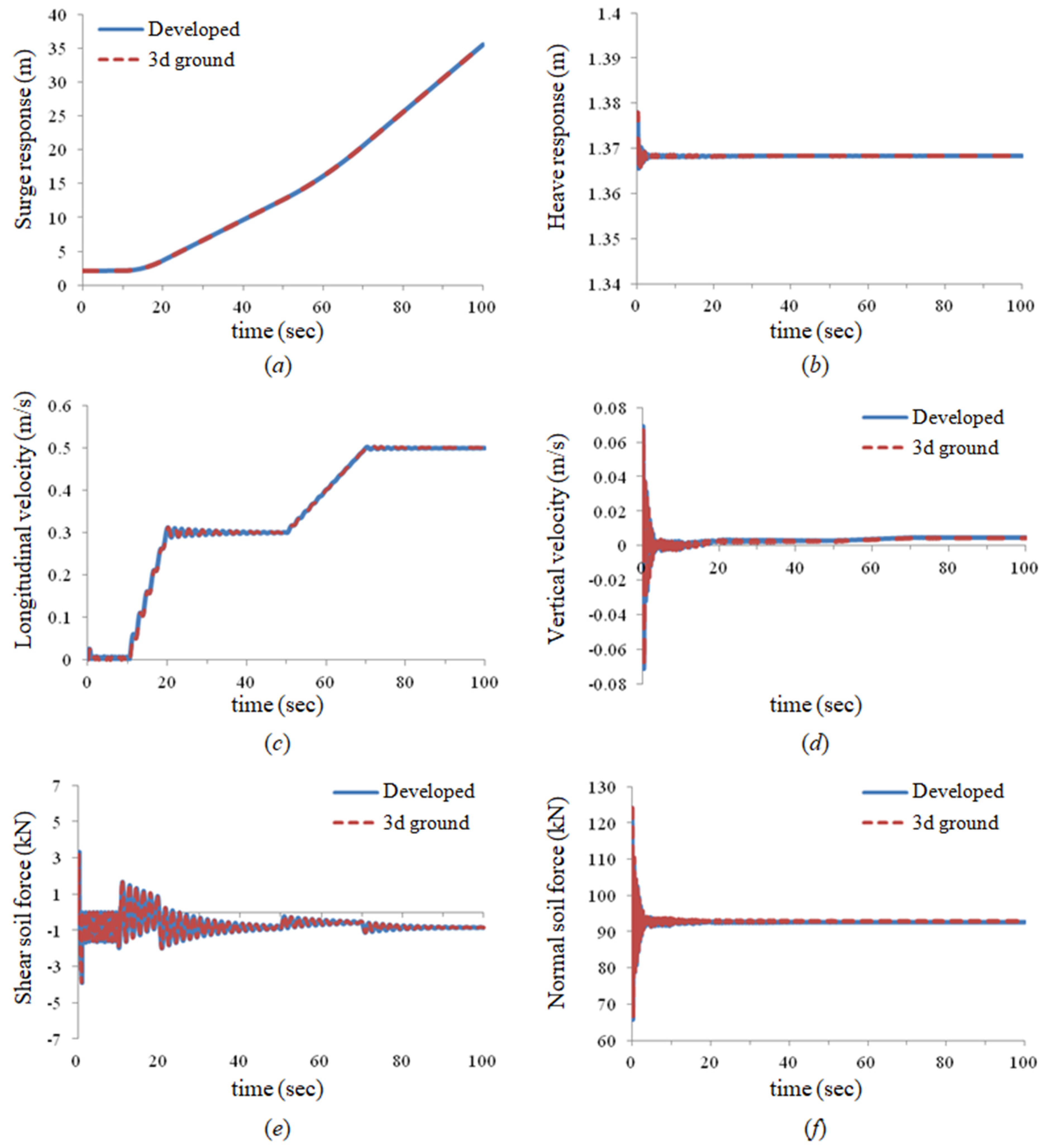
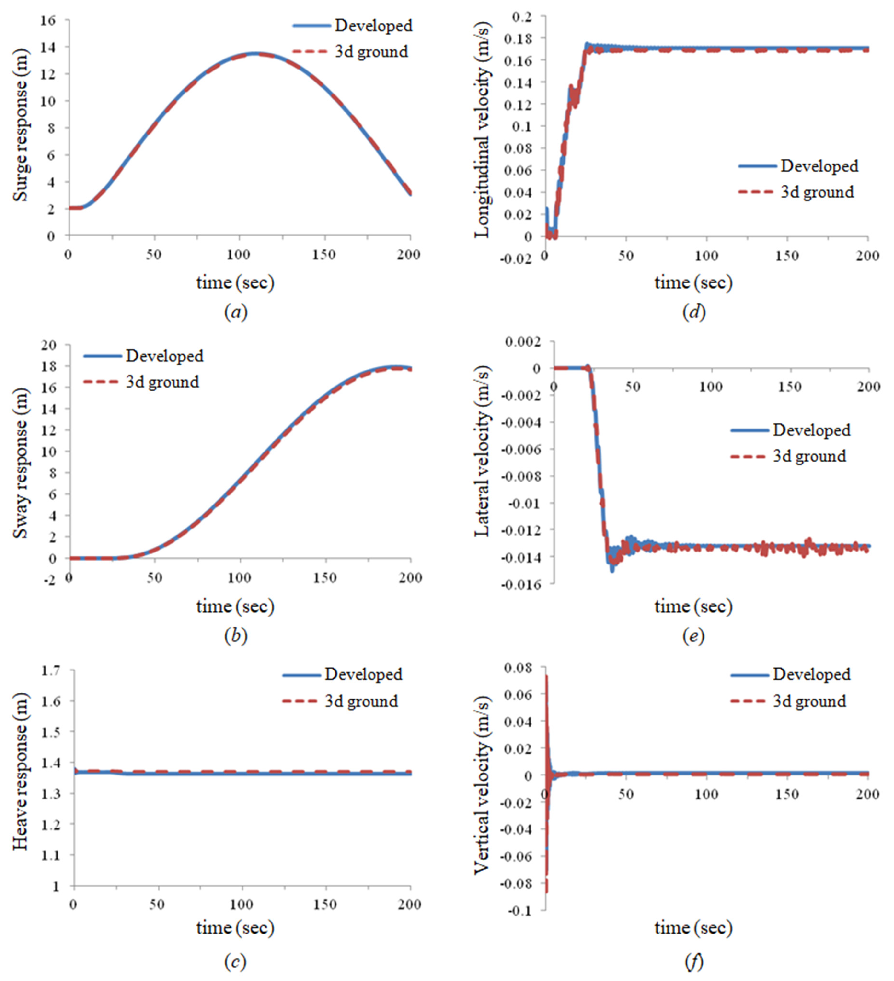
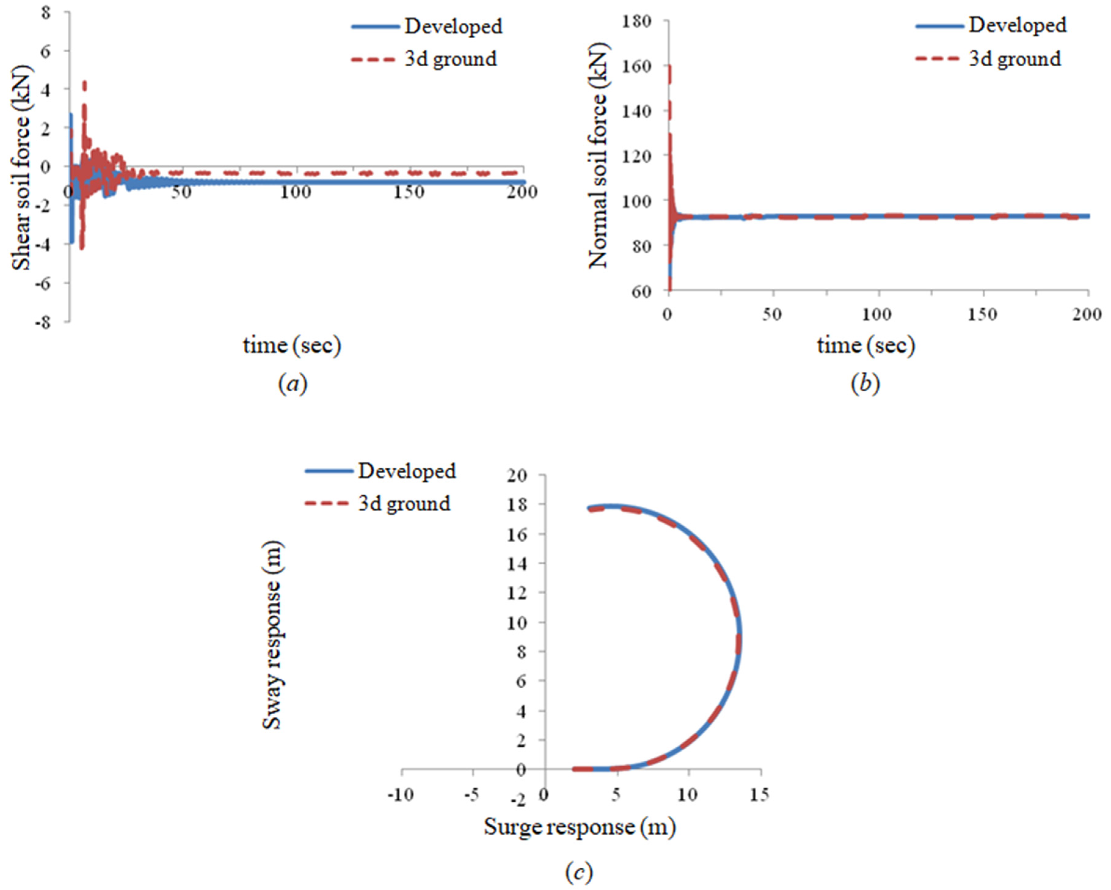
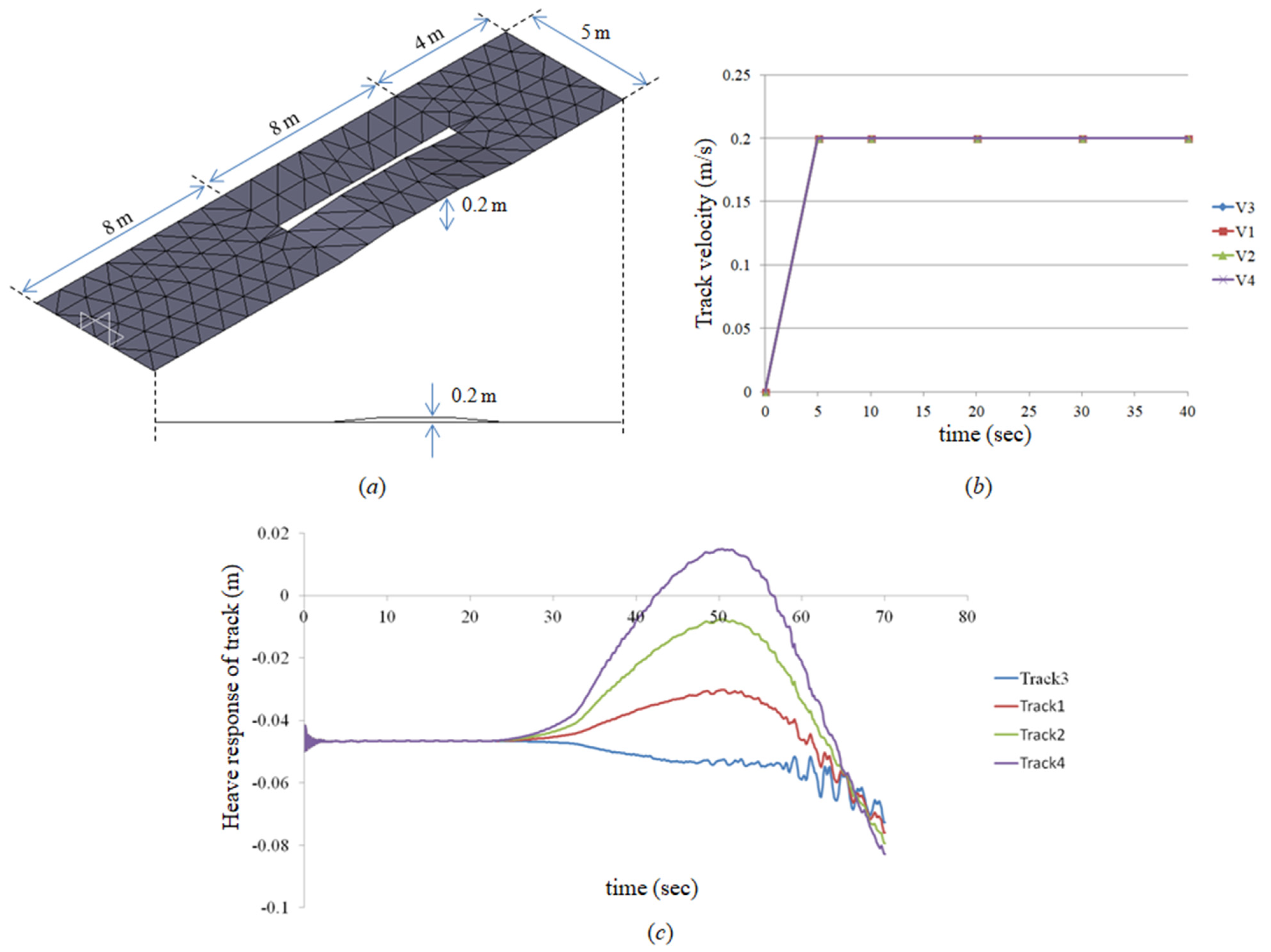
7.3. Three-Dimensional Ground Mechanism for Soil Contact
8. Conclusions
Author Contributions
Funding
Data Availability Statement
Conflicts of Interest
References
- Brink, A.W.; Chung, J.S. Automatic Position Control of a 300,000-Ton Ship Ocean Mining System. J. Energy Resour. Technol. 1982, 104, 285–293. [Google Scholar] [CrossRef]
- Amann, H.; Oebius, H.U.; Gehbauer, F.; Schwarz, W.; Weber, R. Soft Ocean Mining. In Proceedings of the Offshore Technology Conference, Houston, TX, USA, 6–9 May 1991. [Google Scholar]
- Chung, J.S. Deep-ocean Mining: Technologies for Manganese Nodules and Crusts. Int. J. Offshore Polar Eng. 1996, 6, 244–254. [Google Scholar]
- Hong, S.; Kim, K. Proposed Technologies for Mining Deep-Seabed Polymetallic Nodules—Chap 12 Research and Development of Deep Seabed Mining Technologies for Polymetallic Nodules in Korea. In Proceedings of the International Seabed Authority’s Workshop, Kingston, Jamaica, 3–6 August 1999. [Google Scholar]
- Deepak, C.R.; Shajahan, M.A.; Atmanand, M.A.; Annamalai, K. Development Tests on the Underwater Mining System Using Flexible Riser Concept. In Proceedings of the 4th ISOPE Ocean Mining Symposium, Szczecin, Poland, 23–27 September 2001. [Google Scholar]
- Leng, D.; Shao, S.; Xie, Y.; Wang, H.; Liu, G. A brief review of recent progress on deep sea mining vehicle. Ocean Eng. 2021, 228, 108565. [Google Scholar] [CrossRef]
- Bleier, M.; Almeida, C.; Ferreira, A.; Pereira, R.; Matias, B.; Almeida, J.; Pidgeon, J.; Lucht, J.V.D.; Schilling, K.; Martins, A.; et al. 3D Underwater Mine Modelling in the Vamos Project. In Proceedings of the International Archives of the Photogrammetry, Remote Sensing and Spatial Information Sciences, Limassol, Cyprus, 2–3 May 2019. [Google Scholar]
- Kang, Y.; Liu, S. The Development History and Latest Progress of Deep-Sea Polymetallic Nodule Mining Technology. Minerals 2021, 11, 1132. [Google Scholar] [CrossRef]
- Raja, V.; Solaiappan, S.K.; Kumar, L.; Marimuthu, A.; Gnanasekaran, R.K.; Choi, Y. Design and Computational Analyses of Nature Inspired Unmanned Amphibious Vehicle for Deep Sea Mining. Minerals 2022, 12, 342. [Google Scholar] [CrossRef]
- Wu, Q.; Yang, J.; Guo, X.; Liu, L.; Lu, W.; Lu, H. Experimental study on dynamic responses of a deep-sea mining system. Ocean Eng. 2022, 248, 110675. [Google Scholar] [CrossRef]
- Oh, J.-W.; Lee, C.-H.; Hong, S.; Bae, D.-S.; Cho, H.-J.; Kim, H.-W. A study of the kinematic characteristic of a coupling device between the buffer system and the flexible pipe of a deep-seabed mining system. Int. J. Nav. Arch. Ocean Eng. 2014, 6, 652–669. [Google Scholar] [CrossRef] [Green Version]
- Oh, J.-W.; Lee, C.-H.; Hong, S.; Bae, D.-S.; Lim, J.-H.; Kim, H.-W. Study on Optimum Curve Driving of Four-row Tracked Vehicle in Soft Ground using Multi-body Dynamics (in Korean). J. Ocean Eng. Technol. 2014, 28, 167–176. [Google Scholar] [CrossRef] [Green Version]
- Hong, S.; Choi, J.; Yeu, T.; Kim, H.; Kim, S.; Min, C.; Lee, M.; Seong, K.; Lee, C.; Oh, J. Development of buffer station for safe and eco-friendly mining of seabed mineral resources. In Proceedings of the Underwater Mining Institute, Lisbon, Portugal, 21–28 September 2014. [Google Scholar]
- Park, S.J.; Yeu, T.K.; Yoon, S.M.; Hong, S.; Kim, H.W. Development of Operating S/W and DBMS for Deep-sea Manganese Nodule Miner. J. Korean Soc. Oceanogr. 2008, 13, 229–236. [Google Scholar]
- Hong, S. Dynamic Analysis of Riser with Vortex Excitation by Coupled Wake Oscillator Model. J. Korean Soc. Oceanogr. 2000, 13, 237–245. [Google Scholar]
- Hwang, S.; Choi, J.; Yeu, T.; Kim, H.; Kim, S.; Min, C.; Lee, M.; Seong, K.; Lee, C.; Oh, J. Three-Dimensional flow response analysis of subsea riser transporting deep ocean water. In Proceedings of the Underwater Mining Institute, Lisbon, Portugal, 21–28 September 2014. [Google Scholar]
- Haug, E.J. Computer Aided Kinematics and Dynamics of Mechanical Systems Volume I: Basic Methods; Allyn & Bacon: Boston, MA, USA, 1989. [Google Scholar]
- Lee, J.K.; Kang, J.S.; Bae, D.S. An Efficient Real-time Vehicle Simulation Method Using a Chassis-based Kinematic Formulation. Proc. Inst. Mech. Eng. Part D J. Automob. Eng. 2014, 228, 272–284. [Google Scholar] [CrossRef]
- Lim, J.-H.; Jo, S.-C.; Bae, D.-S.; Cho, H.-J. A Jacobian formulation for efficient simulation of multibody chain dynamics. J. Mech. Sci. Technol. 2018, 32, 3745–3754. [Google Scholar] [CrossRef]
- Bae, D.S.; Kim, H.W.; Yoo, H.H.; Suh, M.S. A Decoupling Solution Method for Implicit Numerical Integration of Constrained Mechanical Systems. Mech. Struct. Mach. 1999, 27, 129–141. [Google Scholar] [CrossRef]
- Potter, M.C. Mechanics of Fluids; 3/E: SI Ver.; Cengage Learning: Boston, MA, USA, 2008. [Google Scholar]
- Fossen, T.I. Marine Control System: Guidance, Navigation and Control of Ships, Rigs and Underwater Vehicles; Marine Cybernetics: Trondheim, Norway, 2002. [Google Scholar]
- Kim, H.W.; Hong, S. Hydrodynamic Effects on Dynamics of Test Miner on Soft Deep Seafloor. J. Korean Soc. Precis. Eng. 2007, 24, 19–25. [Google Scholar]
- Hong, S.; Kim, H.W. Coupled Dynamic Analyses of Underwater Tracked Vehicle and Long Flexible Pipe. J. Korean Soc. Oceanogr. 2008, 13, 237–245. [Google Scholar]
- Diebel, J. Representing Attitude: Euler Angles, Unit Quarterions, and Rotation Vectors; Stanford University: Stanford, CA, USA, 2006. [Google Scholar]
- Crandall, S.H. An Introduction to Mechanics of Solids: In SI Units, 3rd ed.; McGrawHill: New York, NY, USA, 2012. [Google Scholar]
- Oh, J.-W.; Min, C.-H.; Lee, C.-H.; Hong, S.; Bae, D.-S.; Lim, J.-H.; Kim, H.-W. Arrangement Plan of Buoyancy Modules for the Stable Operation of the Flexible Riser in a Deep-Seabed Mining System. Ocean Polar Res. 2015, 37, 119–125. [Google Scholar] [CrossRef] [Green Version]
- Kim, H.-W.; Lee, C.-H.; Hong, S.; Choi, J.-S.; Yeu, T.-K.; Min, C.-H. Study on Steering Ratio of Four-Row Rigid Tracked Vehicle on Extremely Cohesive Soft Soil Using Numerical Simulation. J. Ocean Eng. Technol. 2013, 27, 81–89. [Google Scholar] [CrossRef]
- Kim, H.-W.; Min, C.-H.; Lee, C.-H.; Hong, S.; Bae, D.-S.; Oh, J.-W. Dynamic Analysis of Tracked Vehicle by Buoy Characteristics. Ocean Polar Res. 2014, 36, 495–503. [Google Scholar] [CrossRef]
- Ryu, H.S.; Bae, D.S.; Choi, J.H.; Shabana, A.A. A compliant track link model for high-speed, high-mobility tracked vehicles. Int. J. Numer. Methods Eng. 2000, 48, 1481–1502. [Google Scholar] [CrossRef]
- Machado, M.; Moreira, P.; Flores, P.; Lankarani, H.M. Compliant contact force models in multibody dynamics: Evolution of the Hertz contact theory. Mech. Mach. Theory 2012, 53, 99–121. [Google Scholar] [CrossRef]
- Bode, O. Simulation der Fahrt von Raupen-fahrwerken auf Teefseeböden. Ph.D. Thesis, University of Hannover, Hannover, Germany, 1991. [Google Scholar]
- Wong, J.Y. Theory of Ground Vehicles, 3rd ed.; John Wiley & Sons: Hoboken, NJ, USA, 2001. [Google Scholar]
- Kreyszig, E. Advanced Engineering Mathematics, 9th ed.; John Wiley & Sons: Hoboken, NJ, USA, 2006. [Google Scholar]
- Ruan, W.; Liu, S.; Li, Y.; Bai, Y.; Yuan, S. Nonlinear Dynamic Analysis of Deepwater Steel Lazy Wave Riser Subjected to Imposed Top-End Excitations. In Proceedings of the ASME 2016 35th International Conference on Ocean, Offshore and Arctic Engineering, Busan, Korea, 19–24 June 2016. [Google Scholar]
- Oh, J.; Jung, D.; Kim, H.; Min, C.; Cho, S. A study on the simulation-based installation shape design method of steel lazy wave riser (SLWR) in ultra deepwater depth. Ocean Eng. 2020, 197, 106902. [Google Scholar] [CrossRef]


| Parameters | Units | Values |
|---|---|---|
| Outer radius | [m] | 0.2286 |
| Inner radius | [m] | 0.2032 |
| Dry weight | [kg/m] | 270.48 |
| Density | [kg/m3] | 7853.9685 |
| Young’s modulus | [N/m2] | 2.061 × 10¹¹ |
| Poisson’s ratio | [-] | 0.3 |
| Added mass coefficient | [-] | 1.0 |
| Drag coefficient | [-] | 1.2 |
| Parameters | Unit | OrcaFlex | Ruan’s Results | Developed Method |
|---|---|---|---|---|
| Touchdown position | [m] | −1364.183 | −1364.880 | −1370.0 |
| Top tension | [kN] | 3161.277 | 3162.757 | 3104.314 |
| Bottom tension | [kN] | 683.125 | 683.249 | 595.101 |
| Top degree | [deg] | 171.799 | 171.764 | 169.933 |
| Properties | Units | Values |
|---|---|---|
| Robot mass (in air) | [ton] | 27.336 |
| Robot mass (under water) | [ton] | 9.389 |
| Track length | [m] | 4.048 |
| Track width | [m] | 0.7 |
| Number of total track | [EA] | 4 |
| Number of track mesh (length) | [EA] | 33 |
| Number of track mesh (width) | [EA] | 2 |
| Contents | Properties | Symbols | Values |
|---|---|---|---|
| Normal pressure | Pressure | p0 | 11 |
| Pressure coefficient | k1 | 363 | |
| Pressure coefficient | k2 | 440 | |
| Shear pressure | Cohesion | c | 4.4 |
| Internal friction degree | 0 | ||
| Sensitivity | 2.97 | ||
| Shear displacement at the maximum yield stress | 0.44 | ||
| Dynamic sinkage | Dynamic sinkage coefficient | fE | 0.11 |
| Critical pressure coefficient | p_cr | 20 | |
| Dynamic sinkage coefficient | ms | 1 |
| Driving Condition | Contents | Developed Method (Original) | Developed Method (3D Ground) |
|---|---|---|---|
| Straight (100 s) | CPU time | 52.02 s | 74.09 s |
| Memory | 38.32 MB | 38.71 MB | |
| Steering (200 s) | CPU time | 105.89 s | 150.04 s |
| Memory | 41.30 MB | 41.86 MB |
Publisher’s Note: MDPI stays neutral with regard to jurisdictional claims in published maps and institutional affiliations. |
© 2022 by the authors. Licensee MDPI, Basel, Switzerland. This article is an open access article distributed under the terms and conditions of the Creative Commons Attribution (CC BY) license (https://creativecommons.org/licenses/by/4.0/).
Share and Cite
Lim, J.-H.; Kim, H.-W.; Hong, S.; Oh, J.-W.; Bae, D.-S. Simulation Technology Development for Dynamic Analysis of Mechanical System in Deep-Seabed Integrated Mining System Using Multibody Dynamics. Minerals 2022, 12, 498. https://doi.org/10.3390/min12050498
Lim J-H, Kim H-W, Hong S, Oh J-W, Bae D-S. Simulation Technology Development for Dynamic Analysis of Mechanical System in Deep-Seabed Integrated Mining System Using Multibody Dynamics. Minerals. 2022; 12(5):498. https://doi.org/10.3390/min12050498
Chicago/Turabian StyleLim, Jun-Hyun, Hyung-Woo Kim, Sup Hong, Jae-Won Oh, and Dae-Sung Bae. 2022. "Simulation Technology Development for Dynamic Analysis of Mechanical System in Deep-Seabed Integrated Mining System Using Multibody Dynamics" Minerals 12, no. 5: 498. https://doi.org/10.3390/min12050498