Experimental and Numerical Modelling of Deep-Sea-Mining-Generated Turbidity Currents

Abstract

Renewable energy installations and energy storage solutions require significant quantities of critical raw materials such as nickel, cobalt and rare earth metals. The supply chains of these raw materials face many difficulties, such as the continuous decrease of mineral ore grades on land. In view of these complications, the motivation to search for new resources has grown, with the deep sea being seen as a potential source of these minerals. Polymetallic nodule mining generates turbidity currents, which could negatively impact the deep-sea environment. For that reason, we investigate this type of current experimentally and numerically in order to characterize the generated turbidity current. Various non-cohesive sediment types, i.e., different particle sizes, and different concentrations are tested using a lock-exchange set-up. Three sediment types (glass beads, silica sand and a 50/50 blend of glass beads and silica sand) with seven initial sediment concentrations are examined. Additionally, for the numerical work, a drift–flux modelling approach is used to simulate the performed lock-exchange experiments. The results show that the front velocities of the currents resulting from the three sediment types increases with increasing initial concentrations inside the lock regardless. Moreover, using the same initial concentration, the difference in front velocities between the generated currents of the three sediment types decreases as the initial concentration increases. When using an initial volumetric concentration of 2.5% and 3%, the difference in front velocities between the generated current of the three sediment types vanishes. Finally, by comparing the numerical and experimental results, the drift–flux model is proven to be a reliable numerical model for predicting the current.

1. Introduction

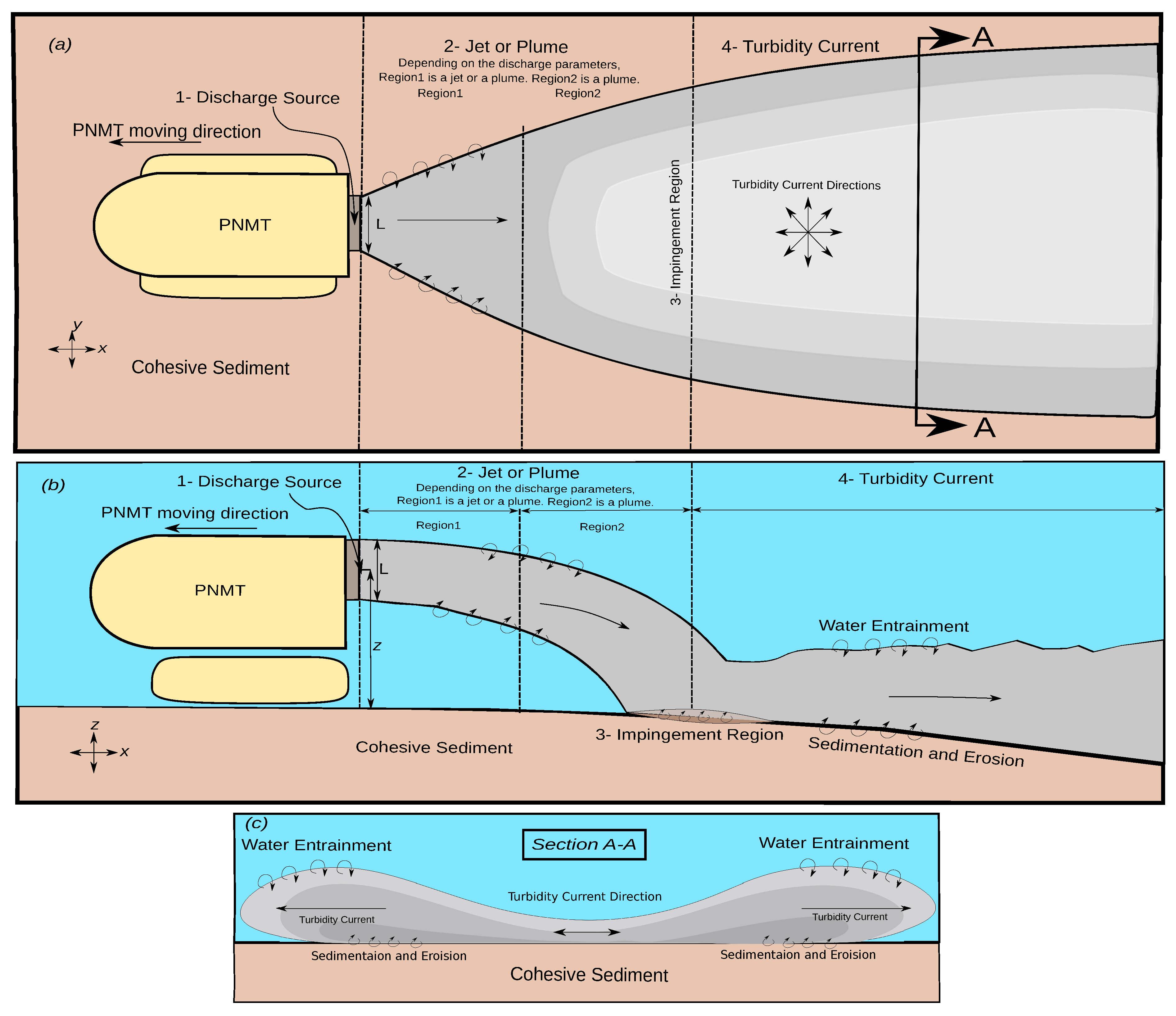
Deep-sea mining involves extracting minerals from the ocean bed, including sulphide deposits, polymetallic nodules and cobalt-rich crusts [1]. In case of polymetallic nodules, a Polymetallic Nodule Mining Tool (PNMT) collects the potato-shaped ore from the ocean bed, after which a primary separation process separates the ore from the excess water–sediment mixture (Figure 1). At the end of the process, the mixture is discharged from the back of the mining tool. The discharged mixture ends up triggering turbidity currents [2], that can significantly alter deep-sea turbidity levels. Keep in mind that not only the discharged mixture affects the surrounding environment but also the disturbances resulting from driving gears such as the wake generated behind the PNMT. According to [3], the negative impact of the generated turbidity current on the environment will result in a change in fauna behaviour and increase the mortality rate of benthic organisms. For that reason, and for the sake of minimizing the affected area by optimizing discharge properties, the present paper focuses on characterizing the different physical parameters (e.g., propagation speed and concentration distribution) that describe a generated current. Moreover, we present our numerical modeling approach that can accurately predict the current.

Overall, gravity currents are characterized by a heavier fluid flowing underneath a lighter fluid, creating a mixing zone in between [4]. Turbidity currents are sediment-laden gravity currents, with forward motion being caused by gravity acting on the density difference between the denser water–sediment mixture and the lighter ambient fluid. Note that the concentration of the suspended sediment within the current is subject to changes throughout the propagation of the current, i.e., sediment deposition, sediment (re-)suspension (erosion) and entrainment of the ambient water.

Generally speaking, turbidity currents are challenging to investigate in the field [5] because of the high cost of the field experiments, and the same applies to mining-generated turbidity currents. However, scaled laboratory experiments are an alternative and widely used option for investigating turbidity currents, with lock-exchange experiments being a particularly simple and useful experimental technique to study turbidity currents [6,7,8,9]. This type of experiments involves suddenly releasing a higher density fluid into a slightly lower density fluid.

Employing lock-exchange experiments, a two-layer shallow-water model including the effect of water entrainment is developed by [10]. Moreover, using an image analysis technique the propagation velocity of the current and concentration profiles are quantified by [11]. Lock-exchange experiments are carried out by [12] to study the effect of bottom roughness on current hydrodynamics. Furthermore, unconfined lock-exchange experiments are also used to study the effect of the lock width on the dynamics of the current by [13].

The effect of particle size on the propagation of turbidity currents is also discussed in literature. The effect of poorly sorted sediments (i.e., wide range of grain sizes) on the deposition behaviour of a turbidity current is investigated by [9,14]. Lock-exchange techniques are also utilized by [6] to examine the effect of bi- and poly-disperse particle mixtures (silicon carbide particles with a particle density of ${\rho }_p=3217$ kg/m³) on the propagation of turbidity currents with a fixed initial volumetric concentration of 0.349% at the lock.

Mathematical and numerical models are also employed to investigate turbidity currents [2,15,16,17,18], but with consideration of a proper validation against field or laboratory experiments. Many numerical studies have been carried out to investigate the characteristics of turbidity currents. Direct numerical simulations are performed for lock-exchange experiments to analyse the structure of the head [16]. The work of [17] presents the effect of the sedimentation on the propagation of the current. Moreover, two- and three-dimensional CFD simulations are used by [18] to investigate the effect of the turbulence vortices on the breakdown of turbidity currents into different sections, i.e., body and tail. Two-dimensional Large Eddy Simulations are performed by [17] to simulate a lock-exchange experiment. Eulerian-Eulerian approach is also used to investigate the effect of particle inertia on current propagation [19]. Additionally, turbidity currents generated in lock-exchange experiments are studied by [20] through LES simulations, comparing the results to an older DNS simulation to assess the quality of this approach.

The well-known Euler–Euler model approaches the turbidity current as separate phases of fluid and solids which are considered interpenetrating continua. From this perspective, the model consists of fluid and solid momentum equations. These equations are coupled by means of source terms [21], which are obtained from the application of the kinetic theory. Mixture models such as the drift–flux model, on the other hand, approach turbidity currents as a single continuum. In other words, the model requires that a single momentum equation to be solved for the mixture as a whole [22,23]. Note that so-called drift velocities are a correction of the “drift” of particles relative to mixture momentum. Many researchers have worked on developing the two-phase drift–flux model, i.e., liquid and single solid phases [22,23,24,25,26]. Recently, a clear mathematical framework for a multiple-phase drift–flux model was presented, where each particle size represents a phase. In this respect, he reported a closure to the relative velocity of the different phases (see Section 4). The main assumptions of drift–flux model are [27]:

(i)

Settling velocity of particles is small compared with the bulk velocity of the mixture;

(ii)

Particles react instantaneously to velocity changes.

The propagation of bi-disperse currents (i.e., two particle sizes are present in the mixture) is investigated by [5], where the lock-exchange experiments done by [6] are simulated and validated by [5] using an Euler–Euler modelling approach.

Beyond the impingement region, the generated turbidity current is directed towards all directions, as shown in the top view in Figure 1. As mentioned before, it is challenging to investigate full-scale generated turbidity currents due to the high costs of the field experiment involved. In order to simplify the process of investigating such a complicated current, we hypothesize that the full-scale turbidity current consists of many small currents next to each other. Taking a small section from a developed mining-generated current such as section A-A in Figure 1, we find that a current generated in a lock-exchange experiment is representative of these small currents in terms of front velocities. In this regard, lock-exchange experiments can be a valuable tool to investigate the effect of different parameters on the propagation behaviour of the current, e.g., initial concentration and particle size. However, it is important to note that the lock-exchange generated currents are not scaled to those generated in mining contexts due to various limitations, such as the free surface area in the lock-exchange experiment and a moving discharge source. We believe that the conclusions drawn from this study will improve approaches to designing the discharge process.

In the present study, we use lock-exchange experiments to investigate the effect of particle size and initial concentration on the behaviour of turbidity currents. We test different initial concentrations for three sediment types with particle densities of ${\rho }_p=2460$ kg/m³ to 2650 kg/m³ which is similar to sediment densities in abyssal plains (see Section 2 for the methodology of the lock-exchange experiments). Moreover, we model the turbidity current by taking multiple fractions into account. Supported by our experimental study, using minimal computational efforts, we aim to demonstrate that the drift–flux model is capable of predicting the main physical parameters (e.g., forward velocity, concentration profiles) associated with turbidity currents. The findings of this paper contribute to defining a discharge framework for mining technology to minimize environmental impact. We present our lock-exchange experimental methodology in Section 2. In Section 3, the experimental results, such as front speed and concentration profiles, are discussed. In Section 4, we describe the numerical methodology based on the drift–flux modelling approach. The numerical results are compared with the laboratory experiments in Section 5. Finally, conclusions are drawn in Section 6.

2. Experimental Apparatus and Laboratory Experiments

2.1. Lock-Exchange Experiments

The lock-exchange experiments are conducted in a rectangular perspex tank with dimensions: $L=3$ m, $W=0.2$ m and $D=0.4$ m. For all runs, the gate is positioned at a horizontal distance of $x_o=0.2$ m (Figure 2). A background plate with white LED strips is installed at the back of the tank. A paper sheet is fixed in front of the white LED strips to generate homogeneous diffused light (Figure 3). A black tent is built around the setup to create a high level of contrast between the tank and the surrounding area. A “IL5HM8512D Fastec” high-speed camera with a Navitar 17 mm lens are used to record video footage of each run (Figure 3). A mixer is used to mix the sediment with the fresh water in the lock (behind the gate at $x_o$) for 1 to 2 min before removing the gate. Three sediment types are tested.

Table 1. Main parameters of the experimental runs.

Runs	Sediment Type	Particle Size Range [$\mathsf{\mu }$m]	Mass [kg]	Volumetric Concentration [%]	Density of Particles [kg/m3]
1	Type1	65–105	0.172	0.5	2460
2	Type1	65–105	0.344	1	2460
3	Type1	65–105	0.517	1.5	2460
4	Type1	65–105	0.689	2	2460
5	Type1	65–105	0.861	2.5	2460
6	Type1	65–105	1.033	3	2460
7	Type2	4–60	0.037	0.1	2650
8	Type2	4–60	0.093	0.25	2650
9	Type2	4–60	0.186	0.5	2650
10	Type2	4–60	0.371	1	2650
11	Type2	4–60	0.557	1.5	2650
12	Type2	4–60	0.742	2	2650
13	Type2	4–60	0.928	2.5	2650
14	Type2	4–60	1.113	3	2650
15	Type3	4–105	0.036	0.1	2460–2650
16	Type3	4–105	0.089	0.25	2460–2650
17	Type3	4–105	0.179	0.5	2460–2650
18	Type3	4–105	0.358	1	2460–2650
19	Type3	4–105	0.537	1.5	2460–2650
20	Type3	4–105	0.715	2	2460–2650
21	Type3	4–105	0.894	2.5	2460–2650
22	Type3	4–105	1.073	3	2460–2650

shows the particle size range, sediment type and density of each type. Type1 sediment consists of round, white synthetic glass beads, Type2 is made up of fine silica sand particles (Millisil M10, irregular particle shape) and Type3 is a mixture of equal parts Type1 and Type2 (50-50 mass). The sediment types were selected to represent a range of particle sizes from coarse to fine. The $D_{10}$, $D_{50}$ and $D_{90}$ for Type1 and Type2 are reported in

Table 2. $D_{10}$, $D_{50}$ and $D_{90}$ in μm for Type1 and Type2.

	D10	D50	D90
Type1	59.09	88.6	132.7
Type2	1.6	17	51

.

The tank is filled with fresh tap water to a depth of $H=0.35$ m for each run. Based on the water volume inside the lock, the required initial concentration is determined by the mass of sediment added in the lock and mixed with the fresh water. The run starts when the gate is suddenly removed, initiating a turbidity current in the tank. The experimental run ends when the current is out of the video boundaries ($L_o=2.4$ m, Figure 3). The propagation of each turbidity current is recorded with a rate of 130 frames per second, 8 bit depth (i.e., number of bits used to define the colour channels).

2.2. Concentration Calibration Method

The same setup (tank and the camera) is used to perform the calibration process. This process begins with filling the mixing section with fresh tap water, after which a pre-weighed mass of sediment is added and mixed. After the water and sediment have been properly mixed, a snapshot is taken of the mixing section. Subsequently, another pre-weighed portion of sediment is added to the mixture and recorded. This process of adding sediment proceeds until the resulting pixel values reach about 255 (i.e., a pixel value of 255 is the camera’s limit for determining different shades of grey, with pixel values ranging from 0 for white to 255 for black, see Figure 4). As a result, every snapshot shows a certain level of concentration.

Table 3. Step-by-step sediment addition and sediment concentration ranges.

Sediment	Concentration Ranges	Increments
Type1	0.0–0.1%	0.01%
	0.1–0.5%	0.05%
	0.5–1.0%	0.10%
	1.0–2.0%	0.25%
Type2	0.0–0.1%	0.01%
	0.1–0.5%	0.05%
Type3	0.0–0.1%	0.01%
	0.1–0.5%	0.05%

shows the concentration ranges and sediment addition steps for each sediment type. For example, Figure 4 shows the calibration process of Type2 sediment, with each snapshot showing a certain volumetric concentration level. The calibration process must be repeated for each sediment type due to differences in the particle reflection index.

The snapshots are identical in terms of length and width, i.e., they feature an equal number of pixels. A Gaussian blur is applied to each snapshot to average the value across the pixel range. Pixels values are not identical across snapshots due to the heterogeneous intensity of the background light. To correct this discrepancy, the pixel value of each pixel is recorded throughout the addition process, following the fact that the pixel indices are fixed in all snapshots. Finally, the concentration-pixel matrix is determined, yielding a calibration curve for each pixel (Figure 5).

2.3. Concentration Measurements

The concentration measurement begins with targeting a specific frame of interest. An algorithm is developed using Python to calculate the concentration. The algorithm proceeds as follows:

• Gaussian blur is applied to the targeted frame.
• The pixel value matrix of the clear water tank frame (the frame taken before opening the lock gate) is obtained.
• The pixel value matrix of the targeted frame is obtained.
• The two matrices of both frames are compared to each other pixel by pixel.
• If a pixel value change is detected between the two frames, based on a pixel value of the clear water tank frame, the concentration–pixel value curve is called.
• From the concentration-pixel value curve (Figure 5), using the pixel value of the targeted frame, the concentration of this pixel is calculated.
• Finally, the targeted frame concentration matrix is calculated, after which the grey scale images are converted into colour maps (red, green and blue) based on concentration values (see Section 3.2 ).

2.4. Front Velocity Measurements

The calculation of the front velocity begins when a distinctive head is formed. An algorithm is developed in Python to calculate the front velocity using a subtraction procedure. The algorithm proceeds as follows:

• The first frame of the recorded video (clear water tank) is obtained.
• The subsequent frames, with a time step of 0.23 s, are subtracted from the first frame in terms of pixel values. Note that the time step represents 30 frames. This number of frames was selected in order to smoothen the distance–time curves.
• The resulting frame from each subtraction step is converted into a binary image with a pixel value of 25 as a threshold.
• The resulting binary image is used to track the front position over time.

3. Experimental Results

This section presents the experimental results and discusses front velocity and concentration maps. In this section, concentration and velocity calculations are based on a two-dimensional approach.

3.1. Front Velocities

One of the most commonly studied quantities in lock-exchange experiments is front speed. According to literature [7,8], based on the front speed, a turbidity current in a lock-exchange experiment exhibits three phases: slumping phase, self-similar phase and viscous-buoyancy phase. The slumping phase occurs near the lock gate, where the dense fluid near the lock starts to collapse. This phase features the formation of a turbidity current front, also known as the head of the current. In this phase, constant propagation speed is observed due to the balance between inertia and buoyancy forces. After the slumping phase, the self-similar phase commences, where the propagation speed of the current is not constant anymore and starts to decrease. Eventually, since viscous forces dominate the flow, the viscous-buoyancy phase is initiated and the current dies out.

Figure 6 shows the measured front positions $x_n$ for all runs as a function of the propagation time t. Velocity instabilities can be observed near the lock gate region, especially with low initial concentrations (i.e., runs 1 and 7). These instabilities are caused by the wave generated by removing the lock gate, since the driving buoyancy force of the low-concentration current might be lower than wave forces. There is an evident positive correlation between the initial concentration and front speed, independent of sediment type. The increase in particle suspension leads to higher buoyancy forces, which provide the current with momentum.

For each sediment type, Figure 7 compares the time needed by the currents as a function of the concentration inside the lock to reach the end of the visualization region. Interestingly, starting from an initial concentration of 1.5% (runs 11, 19) until the end (runs 14, 22), small differences can be observed in front velocity between Type2 and Type3. For initial concentrations of 2.5% (runs 5, 13, 21) and 3% (runs 6, 14, 22), the front velocities are found to be almost the same for all sediment types. Increasing initial concentration strengthens the presence of an important mechanism that increases particles suspension during the development of the current. The resulting high-buoyancy driving forces from the presence of the particles would increase turbulence intensity (i.e., the particles’ gravity forces cannot overcome the turbulence forces, causing the particles to remain suspended). It is therefore obvious that particle size does not play a major role with high concentrations, with the proviso that this may be different for turbidity currents with long run-out distances.

It is challenging to determine the different phases from Figure 6. The work of [7], studying saline gravity currents, showed that the slopes of dimensionless distance–time curves can define the different phases, with the slopes of 1, 2/3 and 1/3 of these curves defining the slumping, self-similar and viscous phases, respectively. To distinguish the different phases in our experiments, the normalized time-distance figures are plotted in Figure 8. The front position $x_n$ is normalized to the lock length $x_o=0.2$, where $X_n=x_n/x_o$ and the time is normalized in accordance with Froude number, where $T=t/(x_o/\sqrt{g_o^{\prime }H})$. Reduced gravity $g_o^{\prime }$ is calculated using the following equation:

$$g_o^{\prime }=\frac{g({\rho }_m-{\rho }_c)}{{\rho }_c},$$

(1)

where g is the the gravitational acceleration, ${\rho }_c$ is water density and ${\rho }_m$ is initial mixture density. The curves shown in Figure 8 are characterized by two distinct slopes: The first slope $\approx 1$ for the slumping phase and second slope $\approx 2/3$ for the self-similar phase. The $1/3$ slope was not observed in any runs, implying that none of the experimental runs made it to the viscous phase. As expected, the slope values for the slumping and self-similar phases follow the findings of [7], since all currents exhibit the slumping phase. After the slumping phase, only run1, i.e., with the lowest initial concentration of Type1 sediment, exhibits the self-similar phase. All runs, except for run1, failed to transition to the self-similar phase. Runs 2–6 of Type1 and run 15–17 of Type3 show that front velocity starts to increase at the end of the visualized region. Nevertheless, no run exhibits a self-similar phase. Moreover, the transition time t* for run1 can be calculated from the intersection between the slopes of 1 and 2/3 of that curve; $t^{*}$ is estimated to be 19.76 s.

The effect of sediment particle size can be observed by examining the dynamics of the currents, with Type2 sediment, consisting of fine particles, revealing no decrease in front velocity. The low particle size and the irregular shapes of Type2 result in low particle settling velocities that cause no decrease in the current’s front velocity. On the other hand, the effect of the coarser particles (in Type1, runs 1–4) is visible at the end of the visualized region, with the coarse particles settling and not contributing to the buoyancy driving forces of the current anymore. For this reason, the curves approach the 2/3 slope line near the end of the visualized region. With Type3, the front velocity observed in runs 15–17 decays at the end because of the deposition of the coarser particles. This can be seen from the slope of the curves, which approach the 2/3 slope. However, for remaining runs of Type3, as mentioned above, the coarser particles did not settle due to high turbulence forces resulting from high driving buoyancy forces. In other words, the curves of the remaining runs have a slope of 1 until the end of the visualization region. In essence, increasing the initial concentration delays the transition time towards the self-similar phase.

3.2. Concentration Distributions

With the calibration process described above, it is possible to measure the concentration of a running current at any time and location, assessing the vertical dispersion of the current. Figure 9 shows colour maps of different snapshots of runs 1, 7–9 and 15–17 acquired at the same front position. The snapshots are taken with the front at the end of the visualized region to ensure the development of the current. The x and y-axes denote the pixel positions. In runs 15–17, currents with type3 sediment have lower concentration distribution values than for Type2 along the whole length of the tank, due to the deposition of large particles. In these specific runs, the settling of coarse particles affects the dynamics of the current during current propagation, whereas the fine particles remain in suspension. Moreover, in run 1, most particles settle and the current is not visible anymore with the used threshold before it reaches the end of the visualized area. For runs 7–9, because of the sediment characteristics of Type2 (i.e., small particle size and irregular particles shape), the particles do not settle during the propagation period of the current. Taking everything into account, only for the runs shown in Figure 9,

(i)

increasing initial concentration leads to higher concentration distribution values and high front speed of the current;

(ii)

increasing particle size reduces the concentration distribution values and the front velocity of the current.

4. Numerical Model Description

In this section, we present a drift–flux model that is used in turbidity current simulations. The drift–flux model is a mixture model where one momentum equation for the whole mixture is required. In this modelling approach, the particles follow the surrounding flow motion but also have a deposition behaviour. In order to justify our choice of drift–flux modeling approach, first, we have to ensure that the particles follow the flow and do not have their own trajectories. Fortunately, Stokes number ($St$) can be used to determine this criterion, where a particle’s Stokes number is the ratio between particle response time ${\tau }_p$ to the flow characteristic time scale $T_k$ of the flow:

$$St=\frac{{\tau }_p}{T_k}=\frac{{\rho }_p{d}_p^2/18\mu }{L/U}$$

(2)

where ${\rho }_p$ is particle concentration, $d_p$ is particle diameter, $\mu$ is the liquid phase dynamic viscosity, L is the characteristic length scale and U is the velocity of the flow at the length scale. In our case, L and U are taken to be the thickness of the current and the front speed of the current, respectively. In case of $St<<1$, this means that the particle response time is much lower than the shortest eddy time scale, which means the particles remain within the flow eddies. If $St>>1$, on the other hand, the particle’s response time is much longer. Consequently, the particle does not follow the eddy. Coarse particles have a high Stokes number. Accordingly, following the experimental results mentioned in Section 3, using the diameter sizes of 60 and 105 μm for runs 6,14 and 22, which the highest front velocity, $St$ is calculated to be $1.3\times {10}^{-3}$, $4.2\times {10}^{-4}$ and $1.2\times {10}^{-3}$, respectively. As such, the drift–flux model is appropriate for this study.

The main assumption of the drift–flux model is that the momentum of solid phases (i.e., each particle size represents a phase) rapidly adapts to the momentum of the liquid phase in a planar direction while continuing to move relative to the liquid phase in the gravitational direction [28]. To put it differently, there is little or no momentum exchange between the solid and liquid phases [27]. This study uses the mathematical multiple-fractions-drift–flux model that was recently reported by [27]. Furthermore, this model is extended in OpenFOAM (an open-source CFD tool). OpenFOAM solves the governing equations sequentially using the Finite-Volume Method (FVM). Accordingly, the equations are integrated at each computational cell, yielding discretized equations for each quantity.

4.1. Governing Equations

The drift–flux model is composed mainly of one mixture momentum equation, one mixture continuity equation and one phase transport equation for each particle size fraction. The mixture continuity equation is defined by the following relationship:

$$\frac{\partial {\rho }_m{\mathbf{u}}_{\mathbf{m}}}{\partial t}+\nabla .{\rho }_m{\mathbf{u}}_{\mathbf{m}}=0,$$

(3)

and the mixture momentum equation can be described as follows:

$$\begin{array}{c}\hfill \frac{\partial {\rho }_m{\mathbf{u}}_{\mathbf{m}}}{\partial t}+\nabla .{\rho }_m{\mathbf{u}}_{\mathbf{m}}{\mathbf{u}}_{\mathbf{m}}=\nabla p_m+\nabla .(({\nu }_m+{\nu }_t)\nabla {\mathbf{u}}_{\mathbf{m}})\\ \hfill -\sum _{k=1}^n{\alpha }_k{\rho }_k{\mathbf{u}}_{\mathbf{km}}{\mathbf{u}}_{\mathbf{km}}+{\rho }_{m}g+M_m,\end{array}$$

(4)

where the subscripts k and m denote the phase k and mixture m, $p_m$ is the mixture pressure gradient, ${\alpha }_k$ is the volume fraction phase k, ${\nu }_m$ is the mixture kinematic viscosity, ${\nu }_t$ is the eddy viscosity, $M_m$ is external source term, ${\rho }_m={\sum }_{k=1}^n{\rho }_k{\alpha }_k$ is the mixture density, ${\mathbf{u}}_{\mathbf{km}}={\mathbf{u}}_{\mathbf{k}}-{\mathbf{u}}_{\mathbf{m}}$ is the relative velocity of the phase k to the mixture m, ${\mathbf{u}}_{\mathbf{k}}$ is the phase velocity and ${\mathbf{u}}_{\mathbf{m}}$ is the mixture velocity and is calculated as follows:

$${\mathbf{u}}_{\mathbf{m}}=\frac{1}{{\rho }_m}\sum _{k=1}^n{\rho }_k{\alpha }_k{\mathbf{u}}_{\mathbf{k}}.$$

(5)

Interestingly, the third term on the right-hand side of equation 4, ${\sum }_{k=1}^n{\alpha }_k{\rho }_k{\mathbf{u}}_{\mathbf{km}}{\mathbf{u}}_{\mathbf{km}}$, is the advection term resulting from the existence of the solid particles. The phase transport equation is given as follows:

$$\begin{array}{c}\hfill \frac{\partial {\alpha }_k}{\partial t}+\nabla .\left({\alpha }_k{\mathbf{u}}_{\mathbf{k}}\right)=\nabla .{\Gamma }_t\nabla {\alpha }_k,\end{array}$$

(6)

$$\begin{array}{c}\hfill \frac{\partial {\alpha }_k}{\partial t}+\nabla .\left({\alpha }_k({\mathbf{u}}_{\mathbf{m}}+{\mathbf{u}}_{\mathbf{km}})\right)=\nabla .{\Gamma }_t\nabla {\alpha }_k.\end{array}$$

(7)

The right-hand side represents the particle turbulence diffusion. ${\Gamma }_t$ is the turbulence diffusion coefficient, which is defined as the ratio between the eddy viscosity ${\mu }_t$ and turbulent Schmidt number $Sc$. In this study, $Sc$ is taken to be 1. Note that we solve the phase transport equation only for the solid phases. To calculate the liquid phase, we use the following:

$$\sum _{k=1}^n{\alpha }_k=1.$$

(8)

Based on that, ${\alpha }_c=1-{\alpha }_t$, where ${\alpha }_c$ is the volumetric concentration of the liquid phase and ${\alpha }_t={\sum }_{k=2}^n{\alpha }_k$ is the volumetric concentration of total solid phases.

Following Equations (4) and (6), ${\mathbf{u}}_{\mathbf{km}}$, ${\nu }_m$, and ${\nu }_t$ require closure. Starting with ${\mathbf{u}}_{\mathbf{km}}$, we employ the following equation using the relative velocity approach [27]:

$${\mathbf{u}}_{\mathbf{km}}={\mathbf{u}}_{\mathbf{kr}}-\sum _{k=1}^n{c}_k{\mathbf{u}}_{\mathbf{kr}},$$

(9)

where ${\mathbf{u}}_{\mathbf{kr}}={\mathbf{u}}_{\mathbf{k}}-{\mathbf{u}}_{\mathbf{c}}$, ${\mathbf{u}}_{\mathbf{kr}}$ is the relative velocity of the phase k to the liquid phase c, which is also known as the terminal settling velocity, and $c_k$ is the mass fraction of phase k. The terminal settling velocity $u_{kr}$ is calculated for each solid phase using the following equation [29]:

$$\begin{array}{c}\hfill u_{kr}=\frac{Rg{d}_p^2}{C_1{\nu }_f+{\left(0.75C_{2}Rg{d}_p^3\right)}^{1/2}},\end{array}$$

(10)

where ${\nu }_f$ is the kinematic viscosity of the liquid phase, g is the gravitational acceleration, $R=({\rho }_p-{\rho }_a)/{\rho }_p$, ${\rho }_p$ is the particle density, ${\rho }_a$ is the liquid phase density, and $C_1$ and $C_2$ are presented in

Table 4. Values of $C_1$ and $C_2$ used for the three sediment types. The typical values of $C_1$ and $C_2$ are 18 < $C_1<24$ and $1<C_2<1.2$.

	Type1	Type2	Type3
$C_1$	18	24	22
$C_2$	0.4	12	1

.

The effect of hindered settling is also taken into account, by using the [30] formula for hindered settling.

$$\begin{array}{c}\hfill u_{kr}=V_m\left({\alpha }_t\right),\end{array}$$

(11)

$$\begin{array}{ccc}\hfill V_m\left({\alpha }_t\right)={(1-{\alpha }_t)}^{e-1}& \mathrm{if}& {\alpha }_t<{\alpha }_{tmax},\hfill \end{array}$$

(12)

$$\begin{array}{ccc}\hfill V_m\left({\alpha }_t\right)=0& \mathrm{if}& {\alpha }_t={\alpha }_{tmax},\hfill \end{array}$$

(13)

where e is the so-called Richardson and Zaki index, which depends on a particle’s Reynolds number that can be defined as the ratio between the particle inertial and viscous forces. We use the empirical equation of [31] to calculate the value of e as follows:

$$e=\frac{a+bR{e}_p^d}{1+cR{e}_p^d},$$

(14)

where $a,b,c,$ and d are experimental coefficients and are taken to be $4.7,0.41,0.175$ and $0.75$, respectively.

The presence of the particles will influence the viscosity. Noting that the mixture is considered in the Newtonian regime, we use the formula of [32] that describes the mixture viscosity as a function of the volume concentration of solids as follows:

$${\nu }_m={\nu }_f(1+2.5{\alpha }_t+10.05{\alpha }_t^2+Aexp\left(B{\alpha }_t\right)),$$

(15)

where A and B are empirical factors that are taken to be $=0.00273$ and $16.6$, respectively [27].

Finally, to calculate ${\nu }_t$ in Equation 4, we use the buoyant $k-ϵ$ model as a closure for turbulence, where k accounts for the turbulence kinetic energy and $ϵ$ for the turbulence energy dissipation rate. The Buoyant $k-ϵ$ model can be described by the following equations [26]:

$$\begin{array}{c}\hfill \frac{\partial {\rho }_{m}k}{\partial t}+\nabla .\left({\rho }_{m}k{\mathbf{u}}_{\mathbf{m}}\right)=\nabla .[({\nu }_m+\frac{{\nu }_t}{{\sigma }_k})\nabla k]+\\ \hfill P_k+P_b+{\rho }_mϵ,\end{array}$$

(16)

$$\begin{array}{c}\hfill \frac{\partial {\rho }_mϵ}{\partial t}+\nabla .\left({\rho }_mϵ{\mathbf{u}}_{\mathbf{m}}\right)=\nabla .[({\nu }_m+\frac{{\nu }_t}{{\sigma }_{ϵ}})\nabla ϵ]+\\ \hfill C_{t1}\frac{ϵ}{k}(P_k+C_{t3}{P}_b)-C_{t2}{\rho }_m\frac{{ϵ}^2}{k},\end{array}$$

(17)

where ${\sigma }_k=1$, ${\sigma }_{ϵ}=1.3$ are the turbulent Prandtl numbers, $C_{t1}=1.44$, $C_{t2}=1.92$, and $C_{t3}=1$ are turbulence model constants. $P_k$ is the generation of turbulence kinetic energy due to mean velocity gradients, and $P_b$ is the generation of turbulence kinetic energy due to buoyancy. It is important to emphasize that, for non-stratified flows, the buoyancy term vanishes where $C_{t3}=0$, while $C_{t3}=1$ in the case of stable stratification. After solving the $k-ϵ$ model, eddy viscosity ${\nu }_t$ can be calculated following this relation:

$${\nu }_t=C_{\mu }\frac{k^2}{ϵ},$$

(18)

where $C_{\mu }=0.09$ is a turbulence constant.

4.2. Application of the Numerical Model

Two-dimensional (2D) computational mesh representing the experimental set-up is shown in Figure 2. A 2D mesh is used further to reduce the computational efforts required. Figure 10 also shows the used Boundary Conditions (B.C); see Section 4.2.1. Two cell zones are defined, with first cell zone 1 representing clear water, i.e., ${\alpha }_c=1$, ${\alpha }_t=0$ and cell zone 2 representing the lock region where ${\alpha }_t$ has a value depending on the initial condition of the numerical run and ${\alpha }_c=1-{\alpha }_t$. The 2D mesh consists of 8000 mesh cells. Furthermore, in both zones, cell dimensions increase in the positive Z direction with a growth rate of 1.02, for the purpose of capturing the dynamics of the current near the bottom in greater detail. The cell dimensions are kept constant in the x-direction (see Figure 10).

4.2.1. Boundary Conditions

In this section, we summarize the general aspects and characteristics of the B.C used in the numerical runs presented here. Boundary conditions are specified for quantities $u_m,p_m,{\alpha }_k,ϵ,k$.

For the velocities ($u_m$), at the free ambient water surface, a slip boundary condition is used. Thus, there are neither convective nor diffusive fluxes present at the top surface, but velocity values are calculated at the boundary. A no-slip condition, i.e., zero velocities at the boundaries, is applied to all solid boundaries of the tank domain. For the pressure $p_m$, a value of 1.013 bar is used at the top surface of the tank to simulate the effect of atmospheric pressure, while zero gradient is used at all tank walls. In addition, the zero gradient for volume fractions ${\alpha }_k$ is assigned to all boundaries of the domain, including the free surface. A zero-gradient boundary condition guarantees that the volume fractions do not escape the domain, and that a bed builds up at the bottom boundary. The presence of walls affects the turbulent flow significantly. In the region near the wall, viscous damping and kinematic blocking reduce normal and tangential velocity fluctuations. Far from the near-wall region, turbulence increases rapidly because of the production of turbulent kinetic energy k. In the current study, wall functions are used for solid boundaries in order to link the viscosity-affected sub-layers between the fully turbulent and near-wall regions. For the free top surface, a zero- gradient BC is used for k and $ϵ$.

4.2.2. Grid Dependency

To investigate the influence of the mesh sizes, front position versus time is depicted for four different computational meshes. Three 2D meshes with 4800, 8000 and 16,800 cells and one three-dimensional (3D)mesh with 60,000 cells are selected to represent coarse, used, fine and 3D meshes, respectively. Experimental run7 is reproduced numerically, using the four proposed computational meshes, and the resulting distance–time figures are plotted in Figure 11. An adjustable time step is used, which means that a new time step is calculated at the end of the previous time step based on the Courant number $C=u\Delta t/\Delta x$. The Courant number represents how quickly information travels along the mesh cells. To have steady numerical runs, we keep C below 1.

The resulting distance–time curves for the four meshes compare very well, which means that the numerical solution can be considered mesh independent. To ascertain the mesh-independence of the solution in more detail, we also calculated the error in two cases: between used/fine meshes and used/3D meshes. Comparing the results of the used and fine meshes, we found that doubling the cell number yields an average difference of 1% in the values of time with respect to distance, while the average difference between the 3D and used meshes is found to be 6.43%. Both are in an acceptable range.

4.3. Number of Used Fractions Sensitivity Analysis

The number of the used fractions in the numerical runs is also a critical factor that can affect the simulation’s accuracy in predicting the parameters associated with a turbidity current. Therefore, we must carry out a number-of-fractions sensitivity analysis to investigate the effect of the used fractions number on the forward velocity of the currents. Run15 is reproduced numerically using number of fractions of 1, 12 and 24. The resulting distance–time curves for the numerical runs and the experimental run are plotted in Figure 12.

The potential energy that the mixture possesses before the gate is removed and the buoyancy forces resulting from the presence of solid particles are the main driving forces of a current. After removing the gate, the potential energy of a mixture transforms directly into kinetic energy. The effect of the kinetic energy on the driving force of the current decreases with time, and buoyancy forces become dominant. Following this understanding, in the first 60 s on the x-axis in Figure 12, front velocity compares well with experimental results because the driving forces were equal in all numerical runs. However, when the effect of the potential energy reduces and buoyancy forces become dominant, a degree of deviation is observed. As a result, beyond 60 s on the x-axis in Figure 12, in the case of 1 and 12 fractions used, a deviation from the experimental result can be observed. This deviation can be attributed to the change in buoyancy forces, since the number of fractions used significantly influences the buoyancy forces. As a result, the 24-fractions run compares well during the whole propagation time of the current, unlike the 1- and 12-fraction runs. Therefore, using a more representable number of fractions of a sediment type in a numerical run will increase the accuracy of a simulated result.

5. Comparison of Numerical Simulations with Experiments

The predictions of the multi-phase drift–flux model are validated in this section. We compare the experimental results to the corresponding numerical results. Runs 1, 7 and 15 are reproduced numerically using the same initial conditions as in the experimental runs. Particle sizes were analysed through PSD testing for each sediment type in order to identify the quantities of each particle size present in the sediment. In addition, 14,12 and 24 fractions are used for Type1, Type2 and Type3, respectively. This information is used to set up the initial conditions of each numerical run.

Figure 13 compares the observed and simulated front position of the current versus time for runs 1, 7 and 15. The numerical model predicts the observed front position very well. This means that the simulations are capable of predicting the three phases of the current, i.e., the slumping, self-similar and viscous phases mentioned in the experimental results, Section 3.

Since it is also important to compare concentration distribution, two snapshots are taken at the same time frame and same front position in both the simulations and the experiments. The first snapshot is taken when the front of the current is almost at the middle of the tank, while the second snapshot is taken when the current reaches the end of the visualized region (see Figure 2). Two concentration profiles are taken per snapshot. For the first snapshot, the first profile is taken at the front of the current, at $\cong 1.6$ m from the lock gate, while the second profile is taken at the body region of the current at a distance of $\cong 0.5$ m from the lock gate. For the second snapshot, the front is taken to be at the end of the visualized region, which is $\cong 2.3$ m from the lock gate and the second profile is at $\cong 1.2$ m from the lock gate. In run 1, only the first snapshot is taken at 24.5 s because the current is unquantifiable when it reaches the last third of the tank. For runs 7 and 15, the first snapshot is taken at 69.5 s and 73.1 s, while the second snapshot is taken at 113 s and 130 s, respectively.

Figure 14, Figure 15 and Figure 16, show the experimental concentration profiles versus the simulated concentration profiles for runs 1, 7 and 15. Generally speaking, the numerical simulations show good agreement with the experimental data. Looking in more detail, a minor degree of divergence is observed between the experiments and simulations in all validation cases, which can be explained by two main factors:

• The use of buoyant $k-ϵ$ turbulence modelling, as this model introduces a degree of inaccuracy to the turbulence calculations.
• The accuracy of the concentration calibration process in the experiments.

Various processes contribute to the turbulence process. One of the most important turbulence damping mechanisms in turbidity currents is damping by buoyancy forces, where solid-particle gravity forces oppose the upward flow fluctuations. This will result in a reduction in kinetic turbulence energy [33]. This mechanism could have a significant effect on the turbulence calculations even in low-concentration currents. Another damping mechanism is the reduction in turbulence kinetic energy due to the change in the effective viscosity, which is why the presence of particles increases the bulk viscosity of the mixture [33].

The standard $k-ϵ$ model was originally developed on the basis of isotropic eddy viscosity and eddy diffusivity models. Accordingly, this model produces good estimations of turbulence calculations in non-stratified flows [34]. With stratified flows (e.g., turbidity currents), the model needs to be tweaked to account for the presence of sediment particles [34]. One of these modifications involves adding a buoyancy damping function term $P_b$ to account for damped turbulence flux resulting from particle buoyancy. Note that this modification was made in the present study (see Equations (16) and (17)). However, our approach still lacks two other damping processes: the turbulence flux of momentum in the vertical direction and the extra vertical mixing between the flow layers due to the particles, i.e., turbulent wake resulting from particle deposition in the vertical direction. These two processes must be modelled in the $k-ϵ$ model. In addition, an accurate estimation of the Schmidt number $Sc={\sigma }_o{F}_m/F_s$ is needed, where $F_m$ is the damping function for momentum, $F_s$ is the damping function for the mixing and ${\sigma }_o$ is the neutral Schmidt number. Normally, the $F_m$ and $F_s$ are calculated as a function of the Richardson number, which is defined as the ratio between buoyancy flux and flow shear (for more on estimating damping functions, see [33]). In addition to damping processes, another possible reason for the observed divergence is the wave at the tank surface caused by removing the lock gate, which is not taken into consideration. Moreover, there is a miss-estimation of the bed formed in the experiments because of the limitations of the calibration process (Section 2.2, Table 3). Keeping this in mind, the deviation between the experimental and numerical calculated concentration distribution at the bottom of the tank, i.e., first 2 cm on the y-axis Figure 14, Figure 15 and Figure 16, can be attributed to the inaccuracy of the measured concentration distribution in the experiments.

To conclude, the damping processes mentioned here and the wave are the reasons for the minor degree of divergence observed in the vertical concentration profiles. However, for the sake of minimizing computational efforts and capturing the general trend of the current without extra costs, we consider that the multiple fractions drift–flux modelling approach can effectively predict the behaviour of a current in a good manner.

6. Conclusions

Particle size plays a major role in turbidity current propagation. In order to quantify turbidity currents generated by mining, this paper investigated the effect of particle size and initial concentration on the propagation of turbidity currents experimentally and numerically. In the following context, the low-concentration turbidity currents and high-concentration turbidity currents are denoted to the currents of $\alpha \le 1\%$ and $1\%\le \alpha \le 3\%$ of the initial concentration, respectively. Note that these conclusions are limited by the tested run-out distance of the current, i.e., the tank length.

• Increasing initial concentrations inside the lock yields high front velocities independent of sediment type. In other words, the transition time to the self-similar phase increases when increasing the initial concentration.
• Increasing particle size leads to low front velocities. With coarse-particle, low-concentration currents, the turbidity current transitions to the self-similar phase more quickly, unlike fine-particle currents that take much longer to transition.
• Increasing initial concentrations neutralizes the particle size effect on current propagation.
• With high-concentration currents, coarse particles have little/no effect on the motion of the current compared to fine-particle currents with the same initial concentration, while in low-concentration currents, coarse particles settle and affect the forward velocity of the current.
• In case of fine-particle, low-concentration currents, low local concentration distribution values are observed during the propagation of the current.
• The new multiple fractions drift–flux model can satisfactorily predict how turbidity currents develop. It is important to remember that the number of fractions used is critical to the accuracy of the predictions, with a greater degree of accuracy being achieved when using a large number of fractions.

These findings can contribute to our understanding of the discharge process from a PNMT. Increasing particle size through flocculation and decreasing the initial concentration at the source might be beneficial in order to minimize environmental impact. Another key point is that the drift–flux model can be utilized to predict the behaviour of turbidity flows behind mining tools. Furthermore, the drift–flux model can be an acceptable choice to optimize the momentum, volume and buoyancy fluxes at the discharge source.

The aggregation-breakup processes that occur between sediment particles during the discharge process and during turbidity current propagation is a matter of importance in any discharge process assessment. However, despite the fact that there are some studies about flocculation processes for deep-sea mininig applications [1,35], a comprehensive understanding of flocculation is still lacking. Moreover, a properly validated numerical model that can predict particle size in the near-field region is still needed.

References

1. Spearman, J.; Taylor, J.; Crossouard, N.; Cooper, A.; Turnbull, M.; Manning, A.; Lee, M.; Murton, B. Measurement and modelling of deep sea sediment plumes and implications for deep sea mining. Sci. Rep. 2020, 10, 5075. [Google Scholar] [CrossRef] [PubMed] [Green Version]
2. Elerian, M.; Alhaddad, S.; Helmons, R.; van Rhee, C. Near-Field Analysis of Turbidity Flows Generated by Polymetallic Nodule Mining Tools. Mining 2021, 1, 251–278. [Google Scholar] [CrossRef]
3. Sharma, R. Environmental issues of deep-sea mining. Procedia Earth Planet. Sci. 2015, 11, 204–211. [Google Scholar] [CrossRef] [Green Version]
4. Chowdhury, M.; Testik, F. Laboratory testing of mathematical models for high-concentration fluid mud turbidity currents. Ocean Eng. 2011, 38, 256–270. [Google Scholar] [CrossRef]
5. Georgoulas, A.N.; Angelidis, P.B.; Panagiotidis, T.G.; Kotsovinos, N.E. 3D numerical modelling of turbidity currents. Environ. Fluid Mech. 2010, 10, 603–635. [Google Scholar] [CrossRef] [Green Version]
6. Gladstone, C.; Phillips, J.; Sparks, R. Experiments on bidisperse, constant-volume gravity currents: Propagation and sediment deposition. Sedimentology 1998, 45, 833–843. [Google Scholar] [CrossRef]
7. Rottman, J.W.; Simpson, J.E. Gravity currents produced by instantaneous releases of a heavy fluid in a rectangular channel. J. Fluid Mech. 1983, 135, 95–110. [Google Scholar] [CrossRef]
8. Huppert, H.E.; Simpson, J.E. The slumping of gravity currents. J. Fluid Mech. 1980, 99, 785–799. [Google Scholar] [CrossRef]
9. Altinakar, S.; Graf, W.H.; Hopfinger, E. Weakly depositing turbidity current on a small slope. J. Hydraul. Res. 1990, 28, 55–80. [Google Scholar] [CrossRef]
10. Adduce, C.; Sciortino, G.; Proietti, S. Gravity currents produced by lock exchanges: Experiments and simulations with a two-layer shallow-water model with entrainment. J. Hydraul. Eng. 2012, 138, 111–121. [Google Scholar] [CrossRef]
11. Nogueira, H.I.; Adduce, C.; Alves, E.; Franca, M.J. Analysis of lock-exchange gravity currents over smooth and rough beds. J. Hydraul. Res. 2013, 51, 417–431. [Google Scholar] [CrossRef]
12. Nogueira, H.I.; Adduce, C.; Alves, E.; Franca, M.J. Image analysis technique applied to lock-exchange gravity currents. Meas. Sci. Technol. 2013, 24, 047001. [Google Scholar] [CrossRef] [Green Version]
13. Lombardi, V.; Adduce, C.; La Rocca, M. Unconfined lock-exchange gravity currents with variable lock width: Laboratory experiments and shallow-water simulations. J. Hydraul. Res. 2018, 56, 399–411. [Google Scholar] [CrossRef] [Green Version]
14. Härtel, C.; Meiburg, E.; Necker, F. Analysis and direct numerical simulation of the flow at a gravity-current head. Part 1. Flow topology and front speed for slip and no-slip boundaries. J. Fluid Mech. 2000, 418, 189–212. [Google Scholar] [CrossRef] [Green Version]
15. Alhaddad, S.; Labeur, R.J.; Uijttewaal, W. Breaching flow slides and the associated turbidity current. J. Mar. Sci. Eng. 2020, 8, 67. [Google Scholar] [CrossRef] [Green Version]
16. Necker, F.; Härtel, C.; Kleiser, L.; Meiburg, E. High-resolution simulations of particle-driven gravity currents. Int. J. Multiph. Flow 2002, 28, 279–300. [Google Scholar] [CrossRef] [Green Version]
17. Cantero, M.; Garcia, M.; Buscaglia, G.; Bombardelli, F.; Dari, E. Multidimensional CFD simulation of a discontinuous density current. In Proceedings of the XXX IAHR International Congress, Thessaloniki, Greece, 24–29 August 2003; pp. 24–29. [Google Scholar]
18. Ooi, S.K.; Constantinescu, G.; Weber, L.J. 2D large-eddy simulation of lock-exchange gravity current flows at high Grashof numbers. J. Hydraul. Eng. 2007, 133, 1037–1047. [Google Scholar] [CrossRef]
19. Henniger, R.; Meiburg, E.; Kleiser, L. Large-Eddy Simulation of Particle-Driven Gravity-Currents. In APS Division of Fluid Dynamics Meeting Abstracts; APS: Melbourne, Australia, 2008; Volume 61, p. GQ-009. [Google Scholar]
20. Garcia, M.H. Depositional turbidity currents laden with poorly sorted sediment. J. Hydraul. Eng. 1994, 120, 1240–1263. [Google Scholar] [CrossRef]
21. Schouten, T.; van Rhee, C.; Keetels, G. Two-phase modelling for sediment water mixtures above the limit deposit velocity in horizontal pipelines. J. Hydrol. Hydromech. 2021, 69, 263–274. [Google Scholar] [CrossRef]
22. Ishii, M. Thermo-fluid dynamic theory of two-phase flow. NASA Sti/Recon Tech. Rep. A 1975, 75, 29657. [Google Scholar]
23. Drew, D.A. Mathematical modeling of two-phase flow. Annu. Rev. Fluid Mech. 1983, 15, 261–291. [Google Scholar] [CrossRef]
24. Zuber, N.; Findlay, J.A. Average Volumetric Concentration in Two-Phase Flow Systems. J. Heat Transf. 1965, 87, 453–468. Available online: https://asmedigitalcollection.asme.org/heattransfer/article-abstract/87/4/453/429617/Average-Volumetric-Concentration-in-Two-Phase-Flow?redirectedFrom=fulltext (accessed on 15 March 2022). [CrossRef]
25. Manninen, M.; Taivassalo, V.; Kallio, S. On the Mixture Model 603 for Multiphase Flow; English; VTT Publications 288; Project Code: 21HIPO Project 604 Code: N5SU00204; VTT Technical Research Centre of Finland: Espoo, Finland, 1996; ISBN 605 951-38-4946-5. [Google Scholar]
26. Van Rhee, C. On the Sedimentation Process in a Trailing Suction Hopper Dredger. Ph.D. Thesis, Delft University of Technology, Delft, The Netherlands, 2002. [Google Scholar]
27. Goeree, J. Drift-Flux Modeling of Hyper-Concentrated Solid-Liquid Flows in 609 Dredging Applications. Ph.D. Thesis, Delft University of Technology, Delft, The Netherlands, 2018. [Google Scholar]
28. Burt, D. Improved Design of Settling Tanks Using an Extended Drift Flux 612 Model. Ph.D. Thesis, University of Bristol, Bristol, UK, 2010. [Google Scholar] [CrossRef]
29. Ferguson, R.; Church, M. A simple universal equation for grain settling velocity. J. Sediment. Res. 2004, 74, 933–937. [Google Scholar] [CrossRef]
30. Richardson, J.; Zaki, W. Sedimentation and fluidisation: Part I. Chem. Eng. Res. Des. 1997, 75, S82–S100. [Google Scholar] [CrossRef]
31. Rowe, P. A convenient empirical equation for estimation of the Richardson-Zaki exponent. Chem. Eng. Sci. 1987, 42, 2795–2796. [Google Scholar] [CrossRef]
32. Thomas, D.G. Transport characteristics of suspension: VIII. A note on the viscosity of Newtonian suspensions of uniform spherical particles. J. Colloid Sci. 1965, 20, 267–277. [Google Scholar] [CrossRef]
33. Toorman, E.; Bruens, A.; Kranenburg, C.; Winterwerp, J. Interaction of suspended cohesive sediment and turbulence. In Proceedings in Marine Science; Elsevier: Amsterdam, The Netherlands, 2002; Volume 5, pp. 7–23. [Google Scholar]
34. Murakami, S.; Kato, S.; Chikamoto, T.; Laurence, D.; Blay, D. New low-Reynolds-number k-ε model including damping effect due to buoyancy in a stratified flow field. Int. J. Heat Mass Transf. 1996, 39, 3483–3496. [Google Scholar] [CrossRef]
35. Gillard, B.; Purkiani, K.; Chatzievangelou, D.; Vink, A.; Iversen, M.H.; Thomsen, L.; Ackley, S.F. Physical and hydrodynamic properties of deep sea mining-generated, abyssal sediment plumes in the Clarion Clipperton Fracture Zone (eastern-central Pacific). Elem. Sci. Anthr. 2019, 7. [Google Scholar] [CrossRef] [Green Version]
Figure 1. Conceptual sketch of the evolution of the sediment–water mixture discharged from a PNMT. (a) Top view of the discharge process from a PNMT; (b) right-side view of the discharge process from a PNMT [2]; (c) section A-A shows the direction of a turbidity current.
Minerals 12 00558 g001
Figure 2. Schematic representation of the tank used in the experiments. The dimensions of the lock and the tank and the water depth are shown.
Minerals 12 00558 g002
Figure 3. (a) Final setup of the tank with the diffused light. The black tent is used to create the maximum contrast; (b) side view of the tank setup showing wooden panel with LED stripes; (c) side view of the LED stripes and the diffused paper in front of it; (d) the high speed/definition camera used in the experiments.
Minerals 12 00558 g003
Figure 4. Shades of grey for Type1 sediment.
Minerals 12 00558 g004
Figure 5. Calibration curve for one of the pixels for Type1 sediment.
Minerals 12 00558 g005
Figure 6. Front position of the turbidity currents x n as a function of the propagation time t.
Minerals 12 00558 g006
Figure 7. Time needed by the current to reach the end of the visualized region as a function of the initial concentrations.
Minerals 12 00558 g007
Figure 8. Log-Log plot of dimensionless time, T, vs. dimensionless front positions for all experimental runs. The solid lines represent the slopes 1 and 2/3 for the long and short lines, respectively. The right figure provides a more detailed look at the transition point of the current from slope 1 to slope 2/3.
Minerals 12 00558 g008
Figure 9. Comparison of the concentration distribution of the currents. The rows represent the same initial concentration and the columns represent the same sediment type. All the runs are acquired at the same front position.
Minerals 12 00558 g009
Figure 10. Geometry, mesh and boundary conditions used in the numerical simulations.
Minerals 12 00558 g010
Figure 11. Grid-dependency study of numerical Run7. The front position of the current is plotted with respect to time for three different 2D meshes and one 3D mesh.
Minerals 12 00558 g011
Figure 12. Sensitivity analysis for the number of the used fractions in the case of numerical run 15. The front position of the current is plotted with respect to time for the number of used fractions of 1, 12, 24 and experimental results.
Minerals 12 00558 g012
Figure 13. Validation cases for runs 1, 7 and 15. Front velocities of the numerical runs are compared to experimental runs.
Minerals 12 00558 g013
Figure 14. Validation case for run1. Vertical concentration profiles are shown for the front and the body of the current. The first snapshot is taken when the front of the current has almost reached the middle of the tank.
Minerals 12 00558 g014
Figure 15. Validation case for run7. Vertical concentration profiles are shown for the front and the body of the current. The first snapshot is taken when the front of the current has almost reached the middle of the tank.
Minerals 12 00558 g015
Figure 16. Validation case for run15. Vertical concentration profiles are shown for the front and the body of the current. The first snapshot is taken when the front of the current has almost reached the middle of the tank.
Minerals 12 00558 g016