Geochemical Fractal Characteristics of Deep-Sea REE-Rich Sediments in the Western Pacific

Abstract

At present, the challenge for geochemical prospecting of deep-sea, rare, earth-rich sediments is the selection of exploration sites. Because of the unpredictability of offshore operations, the distribution and selection of survey line stations face great challenges. In this paper, we study the fact that the concentration distribution of geochemistry in space may be a part of a special complex process, which is called the multifractal. It requires a large number of indexes to characterize its scale characteristics. Based on the multifractal spectrum, 38 geochemical indices in the Pigafetta Basin region of the western Pacific Ocean are divided into three categories. The three indexes are distinguished by the multifractal parameters. The results of multifractals are in good agreement with those of the cluster analysis and principal component analysis. In addition, on the basis of principal component analysis, we further used the multifractal filtering method to extract element anomalies and delineate element enrichment regions. The first principal component clearly represents the potential element enrichment area. The spatial analysis technique and multifractal method proposed in the paper provide a new idea for geochemical prospecting of deep-sea, rare, earth-rich sediments.

1. Introduction

The study area is located in the Pigafetta Basin in the northwest Pacific Ocean (Figure 1). The research samples were obtained in the western Pacific Ocean by the marine geology No. 6 ship using gravity piston cylinder samples. The depth of the basin is about 5000 m–6500 m, and it spreads southeast. The sedimentary strata of Pigafetta Basin are affected by multiple sedimentary discontinuities. Because the basin is surrounded by seamounts, the influence of an undercurrent on the area is relatively weak, and the sedimentary strata are relatively intact. Quaternary sediments are mainly deep-sea clays with great thickness variations. Pliocene strata are relatively complete in this region. Late Miocene strata generally have layers below 6 m. Generally, the deposition rate of deep-sea clay is almost less than 1 mm/ka. However, the deposition rate in this area is relatively high, which may be related to the special topography of the area. Because the basin is surrounded by mountains, more marine debris is transported to the intermountain basin due to turbidity or current, and the provenance is rich. The clay in the sediments is not only dusty clay, which leads to the rapid deposition rate in this area.

There are a lot of rare earth resources in deep-sea sediments [1,2,3]. In the past, mineralogical [4] and geochemical methods [1,3,5,6,7,8] have been used to analyze rare earth-rich sediments. However, they mainly discussed the correlation between REE and mineral content. The range of anomalous enrichment has not been delineated quantitatively. In the past, the multifractal method has been used to extract geochemical anomalies from solid minerals and achieved good results [9,10], but it is rarely used in the Marine field. In this paper, the multifractal technique is applied for the first time in the analysis of geochemical elements in deep-sea sediments in the western Pacific Ocean, which point out the direction of ocean drilling.

2. Methods

Before chemical analysis of deep-sea sediment samples, the samples were dried, crushed, and ground to 200 mesh, dried at 105 °C, and placed in a dryer. The Si, Ti, Al, Fe, Mn, Mg, Ca, Na, K, and P were tested by an X-ray fluorescence spectrometer (Axios XRF) with detection limits of 0.01%–0.1% and a precision RSD ≤ 2%. The sample preparation process of trace and REE is as follows: weigh the sample to about 0.1 g, place the sample in a Teflon solution tank, add 1 drop of ultra-pure water to wet, add 4 mL of 50% HCL, 10mL of HF, and 2 mL of HCLO₄ to shake well, and place the sample in an electric heating plate to heat and dry the solution. Add 4 mL of 50% HCL and shake until fully dissolved. Rinse the wall with ultra-pure water, heat until the solution is clear and bright, cool for about 30 min, and transfer to 25 mL of constant volume. Trace elements (Cu, Co, Ni, Zn, Sr, Ba, and V) were detected by ICP-OES, and other trace elements and REE were detected by ICP-MS with the detection limit of 0.01–0.1 μg/mL and a precision RSD ≤ 2%. All samples were tested in Guangzhou Marine Geological Survey Laboratory (Guangzhou, China). The analysis and test of sediment samples are in accordance with the relevant provisions of the “Geological and Mineral Industry standard of the People’s Republic of China” in the “Geological and Mineral Industry Standard” of the “Geological and mineral Laboratory Testing quality management standards” for quality accuracy and precision monitoring. In accordance with the relevant provisions of quality control and quality assessment in the chemical composition analysis of rock and mineral samples, the original qualified rate of standard samples and internal samples are checked during the analysis.

2.1. Multifractal Spectrum and Simulation Experiments

In terms of space, a multifractal is the mutual entanglement of single fractals. It describes a measure, which is usually expressed in two or three dimensions. If the measure has spatial or statistical self-similarity, it is called a multifractal. The singularity can decompose the defined region into a series of sub-regions of a single fractal. These sub-regions have not only fractal dimensions, but also the singularity of their respective measures. The fractal dimension and singularity of all these sub-regions form the dimension spectral function, f (α).

The histogram method, wavelet method, multiplier method, and moment method are the most common methods in calculating multifractal spectral functions. Although more and more evidence shows that the distribution of element content has fractal characteristics, most studies are based on a small number of data, are limited to a small number of metal elements, and are seldom design oil and gas exploration fields. In view of this, this paper adopts the typical multifractal moment method for analysis.

The moment method is divided into four steps:

• First, build the allocation function, Xq($\epsilon$) = ${\displaystyle \sum }_{n\left(\epsilon \right)}{(\mathrm{x}i{\epsilon }^2)}_i^q$, the mapping graph of q’s mass distribution function, Xq($\epsilon$), and draw the grid size, ε, on the log–log coordinate graph. Where q is any number and represents the statistical moment order of u(ε), x_iε² represents the total amount of metal in the element with the serial number I and length ε. x_i is the taste value of unit i. Here, the analysis results of P₂O₅ are taken as an example. The value of q ranges from −10 to 10 (−10, −9, and −8…). The step size is 1. It can be seen from Figure 3 that the allocation function has a good linear relationship with the step size, and the slope changes accordingly when the q value changes. The line in Figure 3 shows that the q value is −10, −9, …, 0, and …, with the line corresponding to 10.
• The method of calculating the mass index, τ(q), is determined by the mass distribution function. If u($\epsilon$) has multiplicity, the exponential relation Xq($\epsilon$)∝∈^(τ(q)) exists for any q value, and the mass index can be calculated according to the slope between τ and q, as shown in Figure 3.
• The calculation formula of singular index α is: α(q) = $\partial \mathsf{\tau }\left(q\right)/\partial q$.
• Calculate the fractal dimension f(α): f(α) = α(q)q − $\mathsf{\tau }\left(q\right)$.

2.2. Spatial Principal Component Analysis

Principal component analysis (PCA) is made to replace the original indexes by recombining the original indexes with a certain correlation (such as P indexes) into a group of new, comprehensive indexes that are unrelated to each other. Usually, the mathematical processing makes a linear combination of the original P indicators as a new comprehensive indicator. PCA can effectively improve the interpretability of information [11]. In geochemical element analysis, different element combination characteristics can indicate different geological processes, and different geological processes indicate the enrichment process of different elements [12].

F_p = a_1iZX₁ + a_2iZX₂ + … + a_piZX_p

(1)

a_1i, a_2i…, and the a_pi (i = 1, …, and m) are the eigenvectors corresponding to the eigenvalue of the X covariance matrix sigma. ZX₁, ZX₂…, and ZX_p are the standardized values of the original variable. In a practical application, there are often dimensional differences in indicators, so the dimensional influence must be eliminated before calculation, and the data used in this paper will have a dimensional influence when the original data is standardized. For more information on the PCA approach, see Grunsky (2010) [13] and Ueki and Iwamori (2017) [14].

A = (a_ij) p (m = (a₁, a₂, … a_m)),

(2)

R_ai = λ_i a_i,

(3)

R is the correlation coefficient matrix, λ_i and a_i are the corresponding eigenvalues, and there are unit eigenvectors, λ1 ≥ λ2 ≥…≥ λp ≥ 0.

2.3. Multifractal Filtering Analysis

S-A uses the generalized self-similarity in the frequency domain, adopts the integration of spatial analysis and spectral analysis, and adopts the filtering method to select frequency information to restore the spatial pattern and separate the anomaly from the background [9,15,16]. The relation between the spectral density, S, and the area, A, of the wave number set, whose spectral density is greater than S, is:

A(≥S) ∝ S^−ꞵ

(4)

The logarithm of the above formula is taken, and then LgA-LgS is segmentally fitted by the least square method to obtain the power index β, corresponding to the range of different spectral densities. Filter filtering is designed according to the spectral density, so as to achieve the purpose of field separation [17,18].

3. Results and Discussion

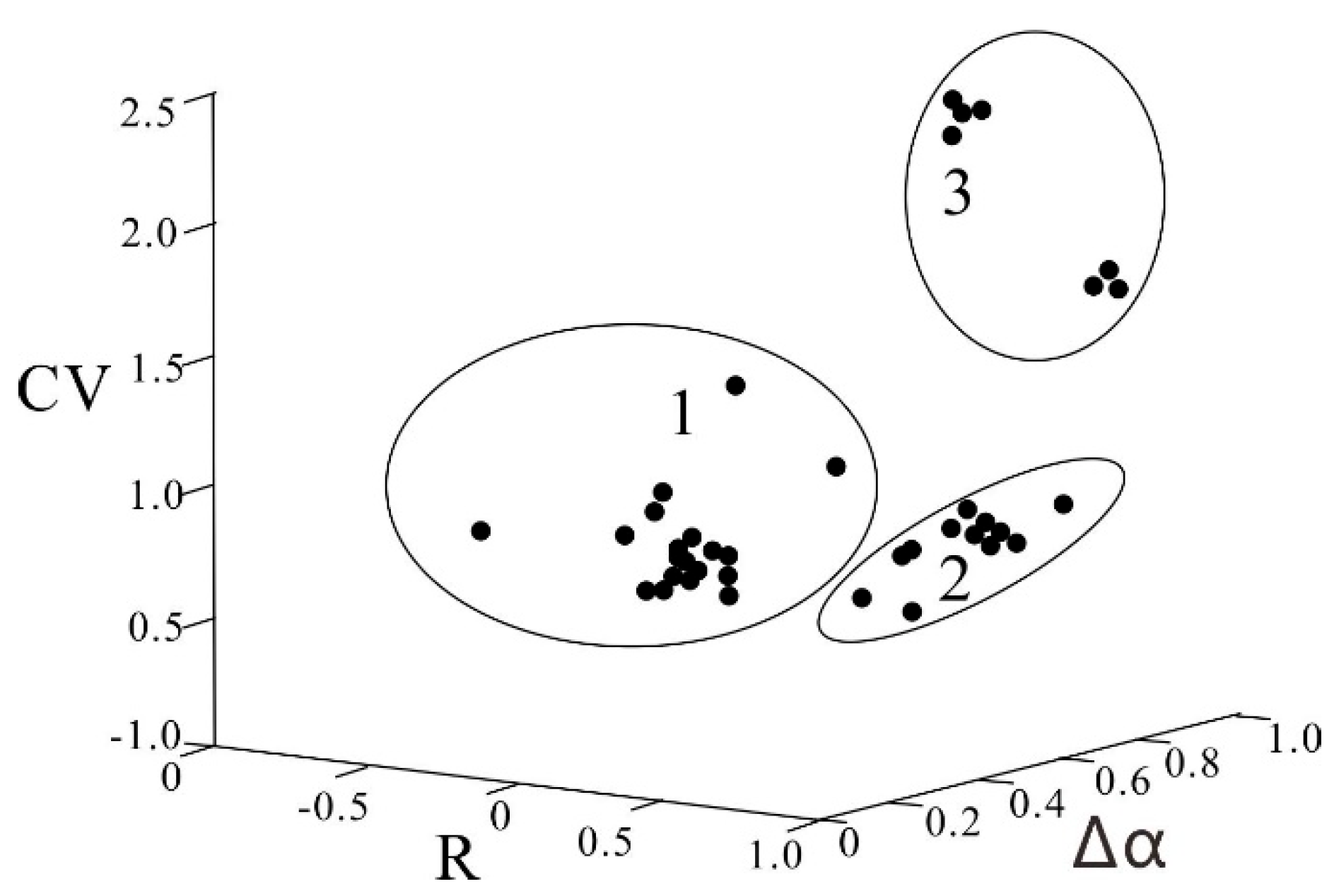
3.1. Statistical Analysis of Samples

Statistical analysis of 3316 samples showed that the original element data set had the following characteristics (

Table 1. The statistical parameters for rare earth elements of 3316 samples from the western pacific.

Elements	Min	Max	Mean	Standard Deviation	Variance	Skewness	Kurtosis	CV%
SiO2	6.53	71.13	49.49	5.09	25.87	−5.18	40.76	10.28
Al2O3	2.26	19.07	15.88	1.82	3.32	−4.61	25.90	11.48
Fe2O3	2.20	19.81	8.62	1.15	1.33	−1.82	9.74	13.40
MgO	0.63	7.29	2.40	0.93	0.86	0.70	0.35	38.66
CaO	1.03	46.53	4.06	4.36	19.00	7.47	60.53	107.44
Na2O	0.10	6.94	2.51	1.61	2.58	0.47	−1.46	64.01
K2O	0.15	4.49	1.51	1.07	1.15	0.45	−1.43	71.22
MnO	0.06	4.05	2.62	1.02	1.04	−0.68	−1.01	38.98
TiO2	0.45	4.80	2.22	1.04	1.08	−0.31	−1.45	46.82
P2O5	0.13	9.99	1.00	0.68	0.46	6.01	52.96	67.38
Co	8.99	556	143.60	48.89	2390.30	0.86	3.45	34.05
Ni	20.50	749	242.70	96.87	9382.95	1.58	4.58	39.91
Cu	45.10	590	355.40	71.00	5041.10	−1.07	2.54	19.98
Zn	25.40	343	155.66	22.21	493.18	−0.80	7.94	14.27
V	34.70	275	160.32	27.18	738.82	−1.43	2.99	16.95
Ba	12.00	4453	178.52	270.84	73353.87	4.39	44.75	151.72
Sc	3.88	1469	48.44	115.47	13332.49	5.94	46.07	238.39
Ga	4.13	86.70	35.71	13.15	172.97	0.19	0.04	36.83
Pb	11.20	358	150.28	86.24	7436.58	−0.40	−1.48	57.38
Sr	19.10	1954	459.97	333.99	111552.29	1.74	3.31	72.61
Cr	20.70	160	72.46	18.83	354.58	−0.45	−0.10	25.99
Zr	39.20	1015	182.80	31.69	1004.55	5.55	149.36	17.34
Y	17.50	1877	173.11	126.00	15875.13	5.33	50.36	72.78
La	13.00	953	102.54	62.42	3896.71	5.52	52.58	60.87
Ce	12.20	1209	114.10	34.98	1223.58	10.70	298.01	30.66
Pr	2.77	263	27.00	17.29	299.06	5.43	51.26	64.06
Nd	12.40	1180	121.69	79.35	6296.30	5.22	48.01	65.21
Sm	2.61	271	26.86	18.01	324.46	5.29	49.05	67.07
Eu	0.76	58.40	6.01	3.95	15.56	5.12	46.44	65.60
Gd	2.67	285	28.66	19.27	371.41	5.15	47.02	67.24
Tb	0.43	47.10	4.62	3.14	9.88	5.36	50.55	68.02
Dy	2.55	268	27.24	18.29	334.52	4.98	44.79	67.15
Ho	0.59	61.40	6.11	4.15	17.22	5.13	47.04	67.93
Er	1.48	164	16.12	10.82	117.14	5.34	50.76	67.16
Tm	0.21	22.50	2.27	1.50	2.26	5.31	49.99	66.25
Yb	1.29	134	13.95	8.94	79.88	5.32	50.68	64.08
Lu	0.19	20	2.08	1.32	1.75	5.36	51.47	63.53
REY	70.76	5983.2	672.36	397.09	157680.99	5.23	48.50	59.06

). Skewness is caused by extreme values in the data set. The frequency distribution of REE is positively skewed, as shown in Table 1, while the skewness degree of P₂O₅ is closest to that of REE, which indicates that the statistical characteristics of REE are very similar to P₂O₅ in the data.

The coefficient of variation (CV) is an important index to evaluate the degree of differentiation of elements. It can be used to statistically characterize the variation of various elements. When CV is greater than 50%, the concentration difference is significant, and the strong differentiation may be due to the fact that the values of these elements may be the result of combined geological processes from a complex genesis. CaO, Sc, and Ba have the largest coefficient of variation, and the corresponding skewness and kurtosis are also larger.

R-type clustering. Classification is carried out according to the degree of correlation between different variables. In the study, if there are many variables and their correlation is strong, the R-type clustering method can be used to cluster the variables into several major categories. There is a strong correlation between the same variables, and the correlation between different variables is low. A typical variable can be found from the same variables as a representative, and the number of variables can be found.

Hierarchical cluster analysis was performed on all elements, and the results were shown in Figure 2. All elements were divided into three categories:

• Ba, Sc, Y, La, Nd, Sm, Eu, Gd, Tb, Dy, Ho, Pr, Er, Tm, Yb, Lu, REY, P₂O₅, Na₂O;
• Co, Ce, Cr, Pb, Ga, SiO₂, MnO, TiO₂, Al₂O₃, Fe₂O₃, Cu, V;
• MgO, CaO, K₂O, Ni, Zn, Sr, Zr.

The first group shows that phosphates are closely related to REE, the second group shows that the iron manganese material, Co, and other metal elements are closely related. REE can be considered to be mainly present in phosphates.

Figure 3 illustrates the process of calculating the multifractal spectrum function of P₂O₅ by the moment method. When constructing the distribution function (Figure 3a), q was set as (−10 and 10) with an interval of one. When ε_s was small, χ_q(ε)-ε showed a straight line. The slope τ(q) of the line was calculated by the least square method, as shown in Figure 3b. The relationship between the singularity index and q value is shown in Figure 3c. Finally, the multifractal spectrum, f(α), was obtained by Lagrange transformation (Figure 3d).

The asymmetry index, R, was first introduced by Xie and Bao (2004) [19] to measure the deviation degree from the symmetric multifractal spectrum curve. R is between −1 and 1. Previous studies [20] used the parameter method to analyze the fractal spectrum function curve, where α₀ is the value of α when q is 0.

Δα_L = |α_min − α₀|

(5)

Δα_R = |α_max − α₀|

(6)

R = (Δα_L − Δα_R)/(Δα_L + Δα_R)

(7)

When R = 0, it means that both sides of the spectral function curve are completely symmetric. R > 0 indicates that the spectral function curve skews to the left; R < 0 indicates that the spectral function curve skews to the right.

Table 2. Multifractal parameter list of chemical elements in the Pijiafeita Basin, in the western Pacific.

	Δα	Δf(α)	[τ(q) − τ(1)]/(q − 1)				ΔαL	ΔαR	R
			q = −10	q = −5	q = 5	Q = 10
SiO2	0.03	−0.18	2.01	2.00	2.00	2.00	0.00	0.03	−0.96
Al2O3	0.02	−0.13	2.01	2.00	2.00	2.00	0.00	0.02	−0.91
Fe2O3	0.01	−0.04	2.00	2.00	2.00	2.00	0.00	0.01	−0.69
MgO	0.03	0.01	2.01	2.01	2.00	1.99	0.02	0.01	0.01
CaO	0.28	−0.64	2.08	2.03	1.94	1.92	0.10	0.18	−0.28
Na2O	0.05	0.14	2.01	2.01	1.99	1.98	0.04	0.01	0.59
K2O	0.09	−0.14	2.03	2.02	1.99	1.98	0.04	0.05	−0.17
MnO	0.18	−0.12	2.14	2.10	1.99	1.99	0.02	0.16	−0.83
TiO2	0.13	−0.40	2.07	2.04	1.99	1.99	0.01	0.12	−0.78
P2O5	0.36	1.22	2.03	2.01	1.96	1.85	0.29	0.07	0.63
Co	0.12	−0.36	2.04	2.01	2.00	1.99	0.02	0.09	−0.59
Ni	0.10	0.07	2.02	2.01	1.99	1.98	0.05	0.05	0.08
Cu	0.01	−0.07	2.00	2.00	2.00	2.00	0.00	0.01	−0.68
Zn	0.00	0.00	2.00	2.00	2.00	2.00	0.00	0.00	−0.02
V	0.03	−0.16	2.01	2.00	2.00	2.00	0.00	0.03	−0.81
Ba	0.07	0.18	2.01	2.02	1.95	1.94	0.08	0.01	0.85
Sc	0.50	1.11	2.03	2.02	1.75	1.65	0.45	0.04	0.82
Ga	0.10	−0.29	2.04	2.02	1.99	1.99	0.01	0.08	−0.69
Pb	0.18	0.04	2.15	2.13	1.99	1.99	0.03	0.15	−0.69
Sr	0.89	−0.71	2.35	2.14	1.97	1.87	0.28	0.61	−0.37
Cr	0.06	−0.33	2.02	2.00	2.00	2.00	0.01	0.06	−0.77
Zr	0.01	−0.01	2.00	2.00	2.00	2.00	0.00	0.00	−0.20
Y	0.34	1.45	2.03	2.01	1.98	1.88	0.29	0.06	0.66
La	0.28	1.38	2.02	2.01	1.98	1.90	0.25	0.03	0.76
Ce	0.09	−0.30	2.03	2.01	2.00	1.99	0.02	0.07	−0.58
Pr	0.32	1.52	2.02	2.01	1.98	1.88	0.28	0.04	0.73
Nd	0.32	1.47	2.02	2.01	1.98	1.89	0.27	0.04	0.72
Sm	0.34	1.58	2.02	2.01	1.98	1.88	0.29	0.05	0.72
Eu	0.33	1.62	2.02	2.01	1.98	1.88	0.29	0.04	0.76
Gd	0.32	1.46	2.02	2.01	1.98	1.88	0.27	0.05	0.70
Tb	0.37	1.69	2.03	2.01	1.97	1.86	0.32	0.05	0.71
Dy	0.30	1.27	2.03	2.01	1.98	1.90	0.25	0.06	0.64
Ho	0.31	1.30	2.03	2.01	1.98	1.89	0.25	0.06	0.64
Er	0.33	1.43	2.03	2.01	1.98	1.88	0.28	0.06	0.66
Tm	0.32	1.40	2.03	2.01	1.98	1.89	0.27	0.05	0.67
Yb	0.30	1.22	2.03	2.01	1.98	1.90	0.24	0.06	0.62
Lu	0.30	1.25	2.03	2.01	1.98	1.90	0.24	0.06	0.63
REY	0.28	1.24	2.02	2.01	1.98	1.91	0.23	0.05	0.66

lists the Δα_L, Δα_R, and R values of spectral functions of each element. According to the results of the R value, we can conclude that the spectral function curve of REE is mainly left-biased.

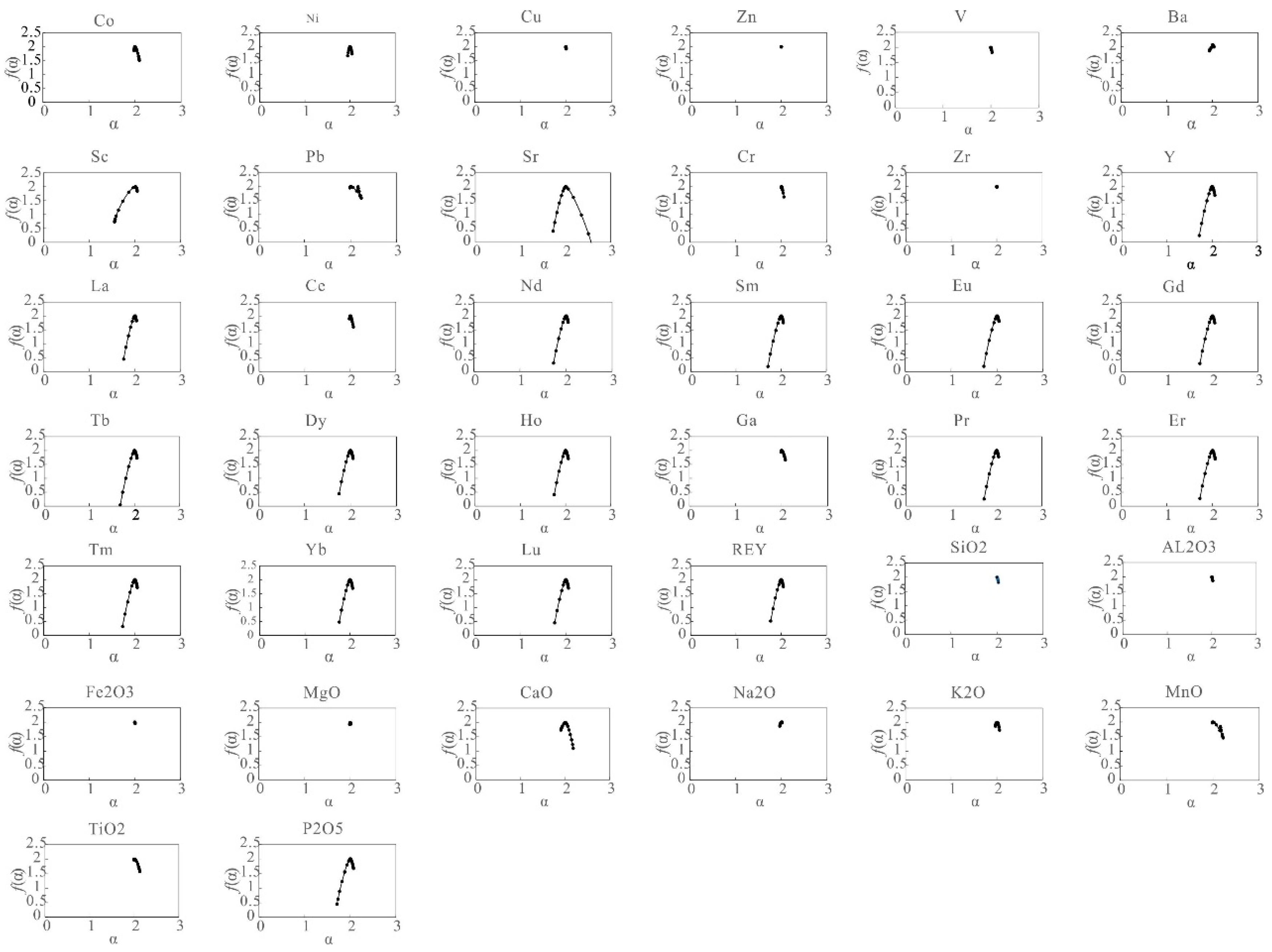
3.2. Multifractal Analysis of REE

These elements were divided into three categories by the analysis of the fractal spectrum curve (Figure 4) and R value:

• Ba, Sc, Y, La, Nd, Sm, Eu, Gd, Tb, Dy, Ho, Pr, Er, Tm, Yb, Lu, REY, P₂O₅, and Na₂O. The Δα group is relatively large, and the corresponding Δf (α) is also large, showing strong multifractal characteristics. The R values of these elements are all greater than 0, and the spectral function curve is biased to the left.
• Co, Ce, Cr, Pb, Ga, SiO₂, MnO, TiO₂, Al₂O₃, Fe₂O₃, Cu, and V. The R values are all less than 0, and the spectral function curves deviate to the right. These indices have a narrow continuous multifractal spectrum curve and show very weak multifractal characteristics.
• The absolute values of R of MgO, CaO, K₂O, Ni, Zn, Sr, and Zr are less than 0.5, indicating a simple single fractal.

In Figure 5, the X-axis is the difference between the maximum value and minimum value of the local singular index of each indicator. The Y-axis is the asymmetric value R, which represents the degree of symmetry deviation from the fractal spectrum, and the Z axis is CV. All elements are divided into three categories.

To further study the relationship between REE and multifractal distribution patterns, dividing each value in P₂O₅ by a constant [21] such as 10, has no effect on the shape of the multifractal spectrum. This indicates that the multifractal spectrum, Δα, and asymmetric index, R, are not affected by the global distortion. The multifractal spectrum is the same, as long as the relatively higher and lower values in the space remain constant. From this point of view, the multifractal spectrum function can effectively reflect the internal spatial structure of the geochemical field of REE. Therefore, Δα, R, and CV, three relatively unchanged parameters, can be used to characterize the inner space characteristics of REE.

Based on the above analysis, the grouping results of 38 geochemical elements by multifractal and statistical analysis are basically consistent.

PCA analysis results of 38 elements in the study area are as follows (Figure 6): (1) Ba, Sc, Y, La, Nd, Sm, Eu, Gd, Tb, Dy, Ho, Pr, Er, Tm, Yb, Lu, REY, P₂O₅, Na₂O; (2) Co, Ce, Cr, Pb, Ga, SiO₂, MnO, TiO₂, Al₂O₃, Fe₂O₃, Cu, V; (3) MgO, CaO, K₂O, Ni, Zn, Sr, and Zr.

Studies have shown that the content of P in deep-sea sediments is the main controlling factor of REE enrichment [22]. Abundant geochemical evidence indicates that REE may be closely related to phosphorus [2,3,5,6]. An analysis showed that P₂O₅ in the study area was positively correlated with Rey (Figure 7), and the correlation coefficient is 0.58. It is also verified that the main carriers of REE in the deep-sea sediments of the western Pacific Ocean are biological phosphates [2,8,23].

The S-A method is applied to multifractal processing of three principal components. In this paper, S-A logarithmic fitting is carried out according to the actual situation of the study area. The dividing point is determined based on the least square method. The basic idea is to calculate the sum of the squares of the difference between the interval fitting data and the original data, namely the sum of the remaining squares. The smaller the sum of the remaining squares, the higher the fitting accuracy. In general, the S-A log–log graph is divided into three fitting lines. In this paper, after comparing the three and four segments, it is found that the fitting accuracy of four segments is higher. Therefore, this paper adopts a 4-section method to separate the abnormal background. Principal component one is divided into four sections, and the four intervals of spectral density are 5–28, 28–646, 646–1173, and 1173–2272, respectively. The slopes of the four straight line segments are 0, −1.32, −2.24, and −2.09, respectively, and the intercepts are 0, 12.32, 18.32, and 17.06, respectively. In order to test the significance of each interval regression equation, an error test was carried out on each equation. The fitting errors of each section are 0, 0.001, 0.001, and 0.002, respectively. Two filters were defined with the threshold of 646: an anomaly filter, S < 646, and a background filter, S > 646. Principal component two is divided into four segments; the energy spectrum densities of four segments are 13–628, 628–1259, 1259–1729, and 1729–1804; the slopes of the four straight segments are −1.27, −1.99, −0.17, and −10.95; and the intercepts are 11.98, 16.69, 3.22, and 83.45, respectively. In order to test the significance of the regression equation of each interval, an error test was carried out on each equation, and the fitting errors of each interval were calculated to be 0.004, 0.007, 0.002, and 0.007, respectively. Two filters were defined with the threshold of 1259: an anomaly filter, S 1259, and a background filter, S > 1259. Principal component three is divided into four segments, and the energy spectrum densities are 5–28, 28–512, 512–807, and 807–1110, respectively. The slopes of the four straight segments are 0, −1.45, −1.51, and −0.18, respectively, and the intercepts are 0, 12.06, 12.37, and 3.02 respectively. In order to test the significance of the regression equation of each interval segment, an error test was carried out on each equation, and the fitting errors of each segment were calculated to be 0, 0.008, 0.006, and 0.002, respectively. Two filters were defined with 512 as the threshold: an anomaly filter, S < 512, and the background filter, S > 512. It can be seen from S-A figure (Figure 8) that this figure always shows a downward trend because as the spectral value increases, the area value of the high spectral value region always decreases. Anomaly filter results mainly reflect the high frequency components of element content, including the local anomaly content of elements and random noise related to interpolation. High values may indicate the enrichment areas of elements and may guide our next exploration direction.

It can be seen that the distribution of high PC1 scores reflects the enrichment area of REE. The distribution of PC1 (Figure 9a) well-summarizes this situation. From this point of view, the distribution of the first group of elements revealed by multifractal analysis mainly reflects the areas of rare earth enrichment. These indexes are regarded as effective auxiliary indexes for rare earth element anomaly delineation.

4. Conclusions

From the perspective of geochemistry, the enrichment of geochemical elements in deep-sea sediments is worth paying attention to, because it has been shown to have fractal or multifractal characteristics on different scales. In this paper, the geochemical indices of deep-sea sediments from the Pijiafeita Basin in the western Pacific Ocean are studied. The classification of geochemical elements in the study area can help deep-sea exploration geochemists better identify useful information of exploration targets. Delineate geochemical anomaly information of deep-sea sediments. Then quantitatively extract comprehensive reservoir evaluation information.

The study concludes that:

• Using multifractal analysis, conventional cluster analysis, and principal component analysis, the sediment samples tend to group according to their geochemical characteristics, i.e., the concentrations of measured elements. They are then divided into three categories. The first group comprises Ba, Sc, Y, La, Nd, Sm, Eu, Gd, Tb, Dy, Ho, Pr, Er, Tm, Yb, Lu, REY, P₂O₅, and Na₂O. The second group comprises Co, Ce, Cr, Pb, Ga, SiO₂, MnO, TiO₂, Al₂O₃, Fe₂O₃, Cu, and V. The third group consists of MgO, CaO, K₂O, Ni, Zn, Sr, and Zr.
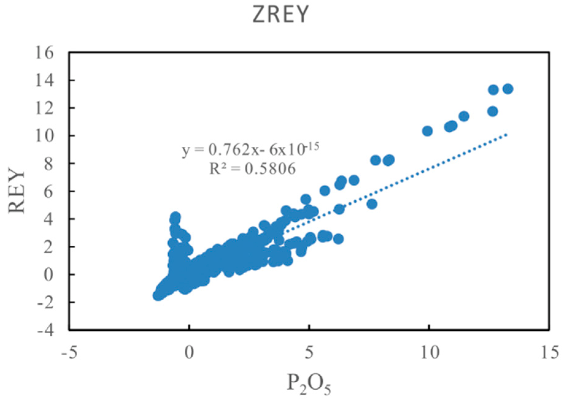
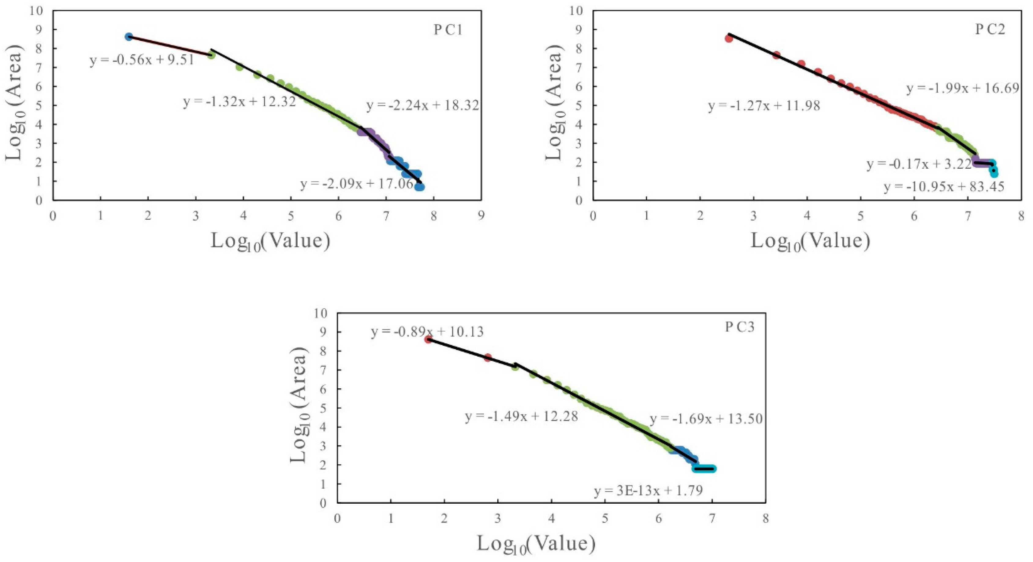
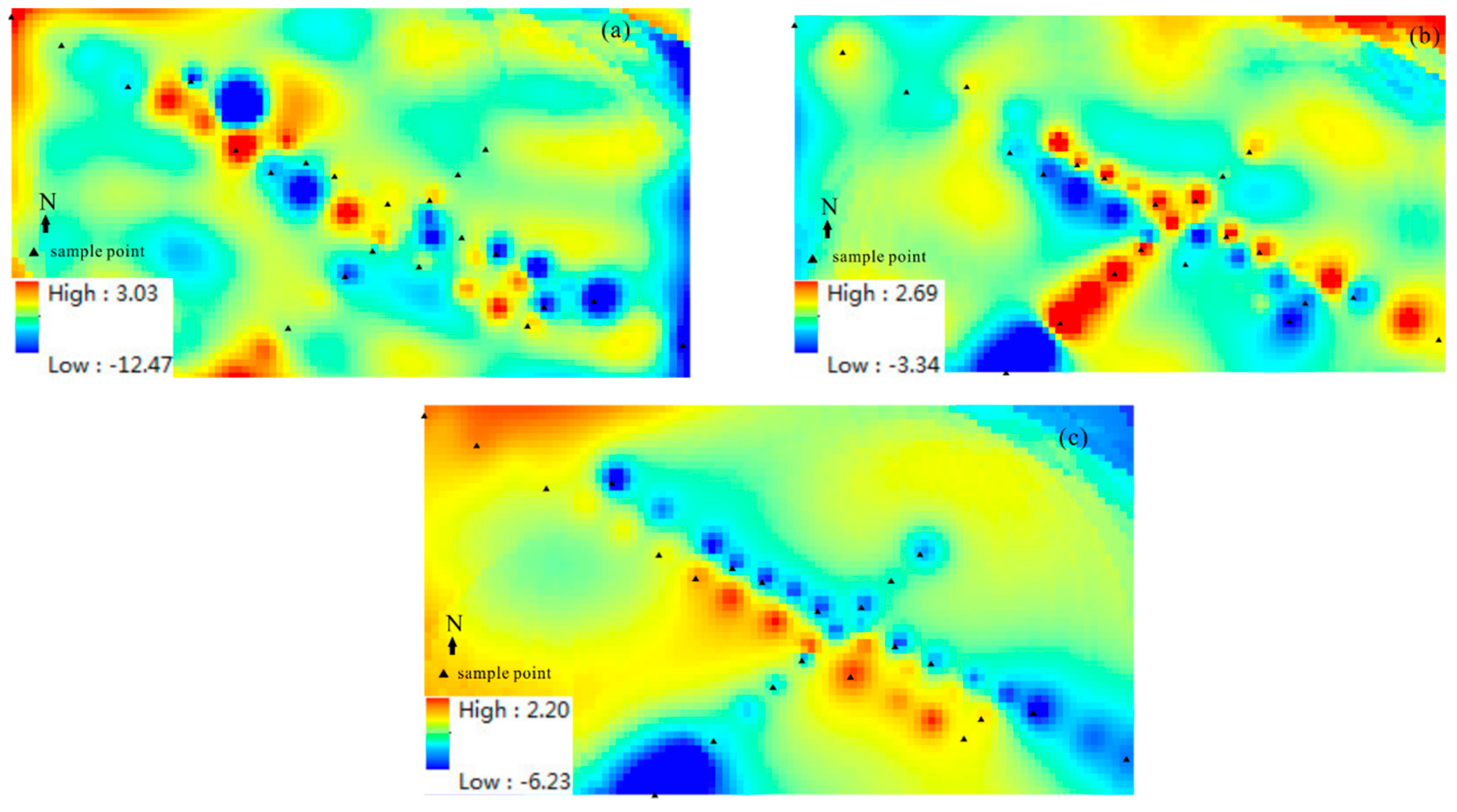
• In order to reduce the number of variables, principal component distribution maps of geochemical elements were compiled based on principal component analysis results, and element enrichment areas were delineated by the S-A multifractal filtering method. The results show that the high content of elements corresponds to the anomaly of the first principal component analysis, represented by Ba, Sc, Y, La, Nd, Sm, Eu, Gd, Tb, Dy, Ho, Pr, Er, Tm, Yb, Lu, REY, P₂O₅, and Na₂O.
• The classification results can provide a new understanding for the delineation of REE anomalies in deep-sea sediments. Understanding these rules can provide quantitative basis for the prediction of REE enrichment and deep-sea resource exploration targets.
• From a new point of view, this paper discusses the resource potential of rare earth in the deep sea. It is proved that surface sediment exploration is not only beneficial to environmental geochemical exploration, and oil and gas geochemical exploration, but it is also beneficial to deep-sea sediment geochemical exploration. Although the statistical analysis of REE enrichment and mineralization in recent years is limited to some extent, this study provides a new idea for the evaluation of deep-sea REE resources.

References

1. Kato, Y.; Fujinaga, K.; Nakamura, K.; Takaya, Y.; Kitamura, K.; Ohta, J.; Toda, R.; Nakashima, T.; Iwamori, H. Deep-sea mud in the Pacific Ocean as a potential resource for rare-earth elements. Nat. Geosci. 2011, 4, 535–539. [Google Scholar] [CrossRef]
2. Yasukawa, K.; Liu, H.; Fujinaga, K.; Machida, S.; Haraguchi, S.; Ishii, T.; Nakamura, K.; Kato, Y. Geochemistry and mineralogy of REY-rich mud in the eastern Indian Ocean. J. Southeast Asian Earth Sci. 2014, 93, 25–36. [Google Scholar] [CrossRef]
3. Emsbo, P.; McLaughlin, P.I.; Breit, G.N.; Du Bray, E.A.; Koenig, A.E. Rare earth elements in sedimentary phosphate deposits: Solution to the global REE crisis? Gondwana Res. 2015, 27, 776–785. [Google Scholar] [CrossRef] [Green Version]
4. Liu, J.H.; Zhang, L.J.; Liang, H.F. The REE geochemistry of sediments in core cc48 from the East Pacific Ocean. Oceanol. Limnol. Sin. 1994, 25, 15–22, (In Chinese with English abstract). [Google Scholar]
5. Kon, Y.; Hoshino, M.; Sanematsu, K.; Morita, S.; Tsunematsu, M.; Okamoto, N.; Yano, N.; Tanaka, M.; Takagi, T. Geochemical characteristics of apatite in Heavy REE-rich deep-sea mud from Minami-Torishima area, southeastern Japan. Resour. Geol. 2014, 64, 47–57. [Google Scholar] [CrossRef]
6. Ren, J.B.; Yao, H.Q.; Zhu, K.C.; He, G.W.; Deng, X.G.; Wang, H.F.; Liu, J.Y.; Fu, P.E.; Yang, S.X. Enrichment mechanism of rare earth elements and yttrium in deep-sea mud of Clarion-Clipperton Region. Earth Sci. Front. 2015, 22, 200–211, (In Chinese with English abstract). [Google Scholar]
7. Zhu, K.C.; Ren, J.B.; Wang, H.F.; Lu, F.F. Enrichment mechanism of REY and geochemical characteristics of REY-rich pelagic clay from the central Pacific. Earth Sci. (J. China Univ. Geosci.) 2015, 40, 1052–1060, (In Chinese with English abstract). [Google Scholar]
8. Wang, F.L.; He, G.W.; Sun, X.M.; Yang, Y.; Zhao, T.P. The host of REE + Y elements in deep-sea sediments from the Pacific Ocean. Acta Petrol. Sin. 2016, 32, 2057–2068, (In Chinese with English abstract). [Google Scholar]
9. Zuo, R.; Wang, J. Fractal/multifractal modeling of geochemical data: A review. J. Geochem. Explor. 2016, 164, 33–41. [Google Scholar] [CrossRef]
10. Zuo, R.; Wang, J. ArcFractal: An ArcGIS Add-In for Processing Geoscience Data Using Fractal/Multifractal Models. Nonrenew. Resour. 2020, 29, 3–12. [Google Scholar] [CrossRef]
11. Cheng, Q.; Bonham-Carter, G.; Wang, W.; Zhang, S.; Li, W.; Qinglin, X. A spatially weighted principal component analysis for multi-element geochemical data for mapping locations of felsic intrusions in the Gejiu mineral district of Yunnan, China. Comput. Geosci. 2011, 37, 662–669. [Google Scholar] [CrossRef]
12. Lei, L.; Xie, S.; Chen, Z.; Carranza, E.J.M.; Bao, Z.; Cheng, Q.; Yang, F. Distribution patterns of petroleum indices based on multifractal and spatial PCA. J. Pet. Sci. Eng. 2018, 171, 714–723. [Google Scholar] [CrossRef]
13. Grunsky, E.C. The interpretation of geochemical survey data. Geochem. Explor. Environ. Anal. 2010, 10, 27–74. [Google Scholar] [CrossRef]
14. Ueki, K.; Iwamori, H. Geochemical differentiation processes for arc magma of the Sengan volcanic cluster, Northeastern Japan, constrained from principal component analysis. Lithos 2017, 290–291, 60–75. [Google Scholar] [CrossRef]
15. Cheng, Q. Spatial and scaling modelling for geochemical anomaly separation. J. Geochem. Explor. 1999, 65, 175–194. [Google Scholar] [CrossRef]
16. Zhang, Y.; Zhou, Y.-Z.; Wang, L.-F.; Wang, Z.-H.; He, J.-G.; An, Y.-F.; Li, H.-Z.; Zeng, C.-Y.; Liang, J.; Lu, W.-C.; et al. Mineralization-related geochemical anomalies derived from stream sediment geochemical data using multifractal analysis in Pangxidong area of Qinzhou-Hangzhou tectonic joint belt, Guangdong Province, China. J. Central South Univ. 2013, 20, 184–192. [Google Scholar] [CrossRef]
17. Ali, K.; Cheng, Q.; Chen, Z. Multifractal power spectrum and singularity analysis for modelling stream sediment geochemical distribution patterns to identify anomalies related to gold mineralization in Yunnan Province, South China. Geochem. Explor. Environ. Anal. 2007, 7, 293–301. [Google Scholar] [CrossRef]
18. Zuo, R.; Xia, Q.; Zhang, D. A comparison study of the C–A and S–A models with singularity analysis to identify geochemical anomalies in covered areas. Appl. Geochem. 2013, 33, 165–172. [Google Scholar] [CrossRef]
19. Xie, S.; Bao, Z. Fractal and Multifractal Properties of Geochemical Fields. Math. Geol. 2004, 36, 847–864. [Google Scholar] [CrossRef]
20. Galuszka, A. A review of geochemical background concepts and an example using data from Poland. Environ. Geol. 2007, 52, 861–870. [Google Scholar] [CrossRef]
21. Zhang, T.; Li, Y.; Chen, Y.; Feng, X.; Zhu, X.; Chen, Z.; Yao, J.; Zheng, Y.; Cai, J.; Song, H.; et al. Review on space energy. Appl. Energy 2021, 292, 116896. [Google Scholar] [CrossRef]
22. Deng, Y.N.; Ren, J.B.; Guo, Q.J.; Cao, J.; Wang, H.F.; Liu, C.H. Geochemistry characteristics of REY-rich sediment from deep sea in Western Pacific, and their indicative significance. Acta Petrol. Sin. 2018, 34, 733–747. [Google Scholar]
23. Zhang, X.; Tao, C.; Shi, X.; Li, H.; Huang, M.; Huang, D. Geochemical characteristics of REY-rich pelagic sediments from the GC02 in central Indian Ocean Basin. J. Rare Earths 2017, 35, 1047–1058. [Google Scholar] [CrossRef]
Figure 1. Sketch map of the location of the study area of the western Pacific.
Minerals 12 00835 g001
Figure 2. Results of cluster analysis of the rare earth elements in the western pacific.
Minerals 12 00835 g002
Figure 3. Process of calculating the multifractal spectral function of P2O5 by the moment method: (a) log–log plot of the mass-partition function vs. the scale length of the cell side for P2O5 concentration values; (b) relation between mass exponents τ(q) and q; (c) and the relationship between singularity exponents α(q) and q; and (d) relation between the multifractal spectrum value f(α) and singularity exponent α.
Minerals 12 00835 g003
Figure 4. Multifractal spectrum curves of the studied elements in the western pacific.
Minerals 12 00835 g004
Figure 5. Verification of the discriminant results based on multifractal parameters Δα and R and CV.
Minerals 12 00835 g005
Figure 6. Results of spatial PCA1 of the 38 elements.
Minerals 12 00835 g006
Figure 7. Cross plots of REY vs P2O5 values.
Minerals 12 00835 g007
Figure 8. Fractal S-A plots (S-A method) for PC1, PC2, and PC3(from left to right). The vertical axis represents cumulative pixel areas, A(r), with PC scores greater than r, and the horizontal axis is the value itself(r). Breaks between straight-line segments and corresponding values of r were used as cutoffs to reclassify pixel values in the multifractal-IDW interpolated map (Figure 9a–c).
Minerals 12 00835 g008
Figure 9. Maps of the distribution of principal components ((ac), the first three principal components) using the multifractal-IDW interpolation method.
Minerals 12 00835 g009