3D Mineral Prospectivity Mapping from 3D Geological Models Using Return–Risk Analysis and Machine Learning on Imbalance Data

Abstract

Three-dimensional Mineral Prospectivity Mapping (3DMPM) is an innovative approach to mineral exploration that combines multiple geological data sources to create a three-dimensional (3D) model of a mineral deposit. It provides an accurate representation of the subsurface that can be used to identify areas with mineral potential. These 3D geological models are the typical data source for 3D prospective modeling. Geological data sets from multiple sources are used to construct 3D geological models. Since in practice there is a significant imbalance in the ratio of mineralized to non-mineralized classes, the classification results will be biased in favor of the more observed classes. Borderline-SMOTE (BLSMOTE) is an oversampling technique used to solve the problem of unbalanced datasets and works by generating synthetic data points along the boundary line between the minority and majority classes. This helps to create a more balanced dataset without introducing too much noise. Non-mineralized samples can be generated by randomly selecting non-mineralized locations, which means that uncertainties are generated. In this paper, we take the shallow-forming low-temperature hydrothermal deposit Guizhou Lannigou gold deposit as an example to extract the ore-controlling elements and establish a 3D geological model. A total of 50 training samples are generated using the sampling method described above, and 50 mineralization prospects are generated using Random Forests. A return–risk analysis was used to explore the uncertainties associated with synthetic positive samples and randomly selected negative samples, and to determine the final mineral potential values. Based on the evaluation metrics G-mean and F-value, the model using BLSMOTE outperforms the model without the synthetic algorithm and the models using SMOTE and KMeansSMOTE. The optimal model BLSMOTE18 has an AUC of 0.9288. The methodology also performs superiorly with different levels of class imbalance datasets. Excluding the predictions where the results highly overlap with known deposits, five target zones were circled for the targets using a P-A plot, all of which have obvious metallogenic geological features. Among them, Target1 and Target2 have good potential for mineralization, which is of great significance for future mineral exploration work.

1. Introduction

Mineral Prospectivity Mapping (MPM) is a geoscientific process that involves assessing and predicting the likelihood of discovering economically viable mineral deposits in a given region. The primary goal of MPM is to identify areas with a higher potential for hosting mineral deposits. This process involves integrating various types of geological, geochemical, geophysical, and remote sensing data, along with an understanding of mineralization processes and geological controls [1,2,3,4,5,6,7,8]. MPM can be subdivided into three types: data-driven methods (such as the evidence weight method, multivariate statistical methods [4]), knowledge-driven methods (such as the Continuous Weighting algorithm [7,9,10]), and hybrid-driven methods [11,12].

Three-dimensional geological modeling techniques have rapidly developed with the advancement of computer technology, 3D geographic information systems, geological statistics, and the mining industry [13,14,15]. Three-dimensional MPM has been widely applied in deep ore prospecting and takes the concept of mapping mineral potential a step further by incorporating the 3D aspect of geological structures and mineralization [12,16,17].

Data-driven MPM refers to the use of ore deposit theories and statistical models to analyze the spatial correlations between known ore deposits and geological features. In the past decade, with the development of computational technology, various machine learning and deep learning algorithms have emerged as the most advanced data-driven MPM methods. Common machine learning methods include Support Vector Machine (SVM), Random Forest (RF), Logistic Regression, and Neural Network [3,6,18,19,20,21,22]. In recent years, deep learning methods have also been introduced into the MPM domain, showing a strong ability to extract mineralized information from complex data structures. Deep learning methods that have been used include: Convolutional Neural Networks (CNN) [23,24,25], Deep Auto-coder (DAE) [26,27], Recurrent Neural Networks (RNN) [28], Long and Short Term Memory Networks (LSTMs) [29], Deep regression networks [30], and Generative Adversariant Networks (GANs) [31].

MPM methods that utilize supervised machine learning typically require positive training datasets and negative training datasets, representing the presence and absence of ore deposits, respectively. Positive training samples can be created based on the known locations of ore deposits. However, research has shown that the mineralization process is a complex system that occurs in anomalous environments, and ore deposits are the result of the coupling of multiple factors at a certain spatiotemporal scale, making them to be considered as rare events [32]. In this geological context, known ore deposits exhibit sparsity, which leads to insufficient positive training samples [18,26,33,34]. The imbalance of the data inevitably affects the accuracy of MPM. Supervised machine learning tends to favor the majority class and ignore the minority class, leading to False Negatives (FN) errors, where positive samples are classified as negative samples [35,36]. Solutions to address the imbalance problem are mainly studied at the classification algorithm level and the data level.

At the classification algorithm level, common methods include cost-sensitive neural networks [35,37], single classifier methods [38,39], semi-supervised/unsupervised algorithms, and ensemble learning methods [26,40]. For example, Zhang et al. [41,42] used Bagging-based PUL (BPUL) to conduct MPM in the Wulong Depression area. Xiong and Zuo [35] applied a cost-sensitive neural network to MPM of the Fe-polymetallic metallogenic belt in southwest Fujian.

On the data level, some strategies are adopted to change the distribution of samples and transform unbalanced samples into a relatively balanced state. Undersampling and oversampling are often used for data resampling. Researchers note that the number of positive samples equal to the number of negative samples in the training set is optimal [43,44,45]. For example, Hariharan et al. [20] use the Synthetic Minority Oversampling technique (SMOTE) to produce a more balanced dataset. The synthetic sample also introduces uncertainty. The study of Li Tongfei et al. [46] showed that the change in the oversampling rate would affect the final result of MPM. In this study, we modify the original training set using the advanced method, Borderline-SMOTE, to balance positive and negative samples.

The selection of negative training samples is also challenging. Many scholars have proposed methods for generating negative training samples, such as those far away from known deposits, other types of known deposits, or random locations [21,47]. However, the study of Zuo and Carranza [18] shows that the selection of negative samples can affect the performance of MPM. At the same time, not all non-metallogenic locations are selected as negative samples, which means that the creation of negative sample datasets introduces uncertainty. However, only a few studies have quantified both the occurrence probability and uncertainty of MPM (e.g., [48,49,50,51]). Resolving this uncertainty is challenging. Because there are no other types of deposits in the study area and there is a high level of drill engineering, this study chose to create negative samples using random non-mineral locations, reducing the risk of introducing bias into the model. Different sets of negative samples have different effects on the results, and in this paper 50 random negative sample sets were created. This variety can help the model generalize better and reduces the uncertainty that can arise from overfitting a specific set of negative samples.

This article proposes a framework for data-driven MPM utilizing machine learning from a three-dimensional geological model. Addressing the issues of data imbalance and uncertainty in negative sample selection, the framework employs the random selection of negative samples and the BLSMOTE technique to generate positive samples for creating the training dataset. The return–risk analysis is utilized to quantify the uncertainty. The RF algorithm is employed for constructing the 3DMPM model of the gold deposit. The practicality of this framework is demonstrated using the case study of the 3DMPM of the Lannigou gold deposit in Guizhou Province.

2. Study Area and 3D Geological Models

2.1. Geological Setting of the Study Area

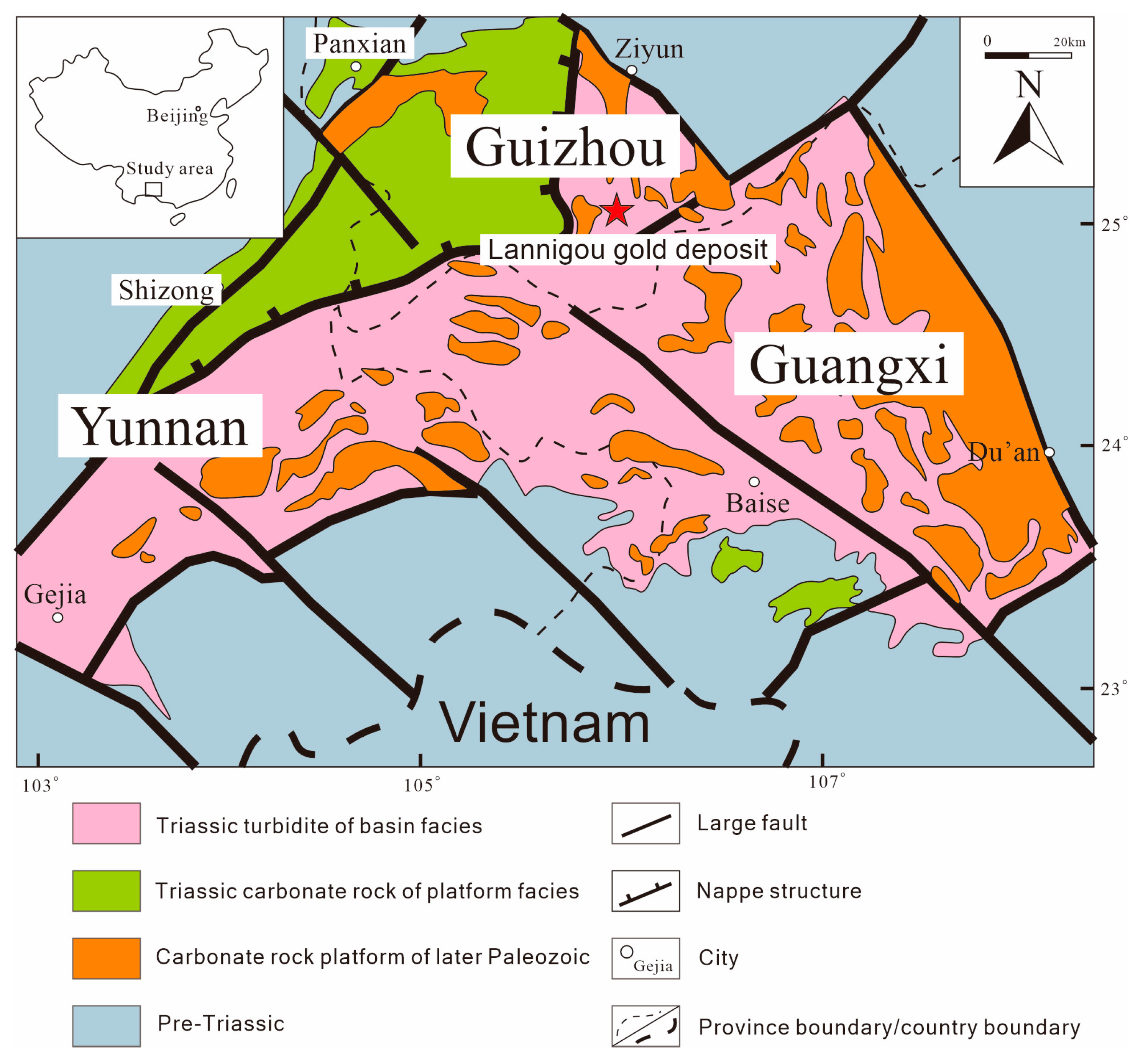
The Lannigou gold deposit is located in the junction of the southwest margin of the Yangtze para-platform and Youjiang Basin, which belongs to the back-arc extensional basin of Lingnan Island, namely the Youjiang fold belt (Figure 1). This area is roughly bounded by the Maitreu-Shizong fault zone, Yadu-Ziyun fault zone, and Kaiyuan-Pingtang fault zone, which constitute the gold deposit concentration area in southwest Guizhou and has good prospective prospect. The mineral resources in the area are dominated by fine-grained disseminated gold deposits, and there is arsenic, mercury, antimony, and other minerals associated with gold deposits (points) or that are independent.

In the west of the mining area, carbonate rocks of Permian shallow water platform facies are found, including the middle Permian Qixia Formation and Maokou Formation, Upper Permian Wujiaping Formation and platform margin reef-beach facies deposits-reef limestone. In the eastern part of the mining area, terrigenous clastic rocks of Triassic trough basin facies are widely exposed, including the Lower Triassic Luolou Formation, Middle Triassic Xuman Formation, Nilo Formation, and Bianyang Formation, with turbidite characteristics, which is the main gold-bearing horizon in the area.

Faults and folds are the most developed in this area, and the faults are mainly divided into three groups: NE trending, NW trending, and NW trending. Fold structure controls the distribution of ore deposits in this area together with large fault structures, while secondary fault structures control the emplacement space of ore deposits. The secondary structural unit belongs to the west side of the NW Wangmo tectonic deformation area and borders the Pu‘an torsional tectonic deformation area in the west. The deposit occurs at the northern apex of the triangular tectonic deformation zone formed by the NE-trending Laizishan anticline, the Luofan extensional fault, the NW trending Banchang thrust fault and the EW-trending Sheheng tectonic belt [52,53,54].

Magmatic activity is weak in the area, and magmatic rocks are mainly distributed in the northeast direction of Zhenfeng County, showing a small-scale mafic and ultrabasic dike, mainly porphyritic and porphyritic pyroxite.

The main types of gold-bearing rocks in the area are sandstone and claystone. Sandstones include fine sandstone, siltstone, and clayey siltstone, and claystone includes claystone and silty claystone. All kinds of ore-bearing rocks have been subjected to intense tectonic fragmentation and different degrees of dynamic hydrothermal metamorphism, which have changed the appearance, internal structure, and even material composition of the original rocks to a large extent, resulting in the formation of cataclastic rocks, porphyry, brecciation, and gouge. The rocks are interspersed by hydrothermal quartz, carbonate veins, and mesh veins, resulting in metasomatic residual erosion and mineralization alteration such as pyrite, calcite, and illytization.

2.2. Ore-Controlling Factors

Geological elements related to mineralization should be extracted before building a 3D geological ore search model [55]. The theory of mineralization systems analyzes the geological and mineralization factors that control the formation, change, and preservation of mineral deposits, including the tectonic system, fluid system, and deposit mechanism [6,56,57]. On this basis, we determined the geological anomaly-controlling factors related to mineralization and established an ore-finding model (

Table 1. Ore controlling factors of the Lannigou gold deposit.

Ore Controlling Factors	Description of Factors	3D Models
Fault	The fault structures provide favorable pathways for the migration of ore-forming fluids.	Regional fault model and fault distance model.
Strata	Ore-bearing strata exhibit distinct trends.	Stratigraphic model.
Hydrothermal solution	Shallow, low-temperature hydrothermal deposits show coexistence and development of Au with As, Sb, and Hg.	Regional geochemical model.
Gathering and protecting	Mineralization occurs in favorable combinations of lithology and intersectional faults.	Geological complexity model and resistivity geophysical model.

). Predictors are provided for the machine learning ore-finding model.

The results of previous studies show that tectonics has a clear control on the location of gold deposits in the study area. Several deep fractures in the area provide upward transportation channels for deep magmatic activity. On the deposit scale, almost all ore bodies are strictly controlled by the fracture structure. The fracture structure provides a good channel for the transportation of metallogenic fluids, and at the same time, in the process of fracture movement, a series of tensional faults will be generated, which provides a good space for mineralization. Therefore, the fracture model and the fracture distance model are used in this paper to jointly describe the regional fracture characteristics.

The survey results show that the ore-bearing strata in the study area are mainly Permian and Triassic strata. The stratigraphically controlled ore bodies are mainly controlled by the impure chert of the Middle Permian Maokou Formation and the unconformity between siltstone and claystone of the Upper Permian Longtan Formation. Fracture-controlled ore bodies are mainly controlled by high-angle faults in the Triassic strata. Therefore, stratigraphic modeling is crucial in the search for ore.

Au, As, Hg, and Sb deposits occur in the Qianxinan Ore Concentration. Gold deposits are mostly produced in the range of the low-temperature hydrothermal mineralization belt of As, Hg, and Sb. Gold deposits are mostly distributed in the vicinity of As, Sb, and Hg ore fields or deposits. They are spatially characterized by close co-(associated) development. According to the results of geochemical aqueous sediment measurements and some rock geochemical measurements, the area is basically characterized by high backgrounds of Au, As, Hg, and Sb. By studying the relationship between different elements and Au, it is possible to determine the ore-finding indicator elements and reveal the enrichment pattern of Au.

Another characteristic of ore body hosting in the study area is that high-grade and large-scale ore bodies are more likely to form at the intersection of faults [52]. In conjunction with the stratigraphic control of mineralization, mineralization occurs in a favorable combination of lithology and intersecting faults. Geological complexity models can be used to depict such geological anomalies. In addition, resistivity geophysical models can be used to analyze stratigraphic development and tectonic morphology, which can be used to enhance the reliability of predictive models.

2.3. The 3D Evidence Layers of Geological Modeling

The geoscientific datasets utilized for regional scale geological modeling and gold deposit modeling are shown in

Table 2. Geosciences dataset for 3D deposit-scale geological modeling.

Data	Number	Description
Geological map	1	1:10,000-scale geological map; strike/dip measurements of surface structural elements.
Drill holes	635	Depth varies from 75 m to 1266 m, with an average depth of 403 m, containing 11,339 stratigraphic data and nearly 300,000 geochemical data.
Geological profiles	40	1:1000-scale geological profiles at an average depth of 400 m.
2D RT inversion maps	16	1:5000-scale average line length of 3875 m, data effective depth of 4000 m, point spacing of 60 m.
Surface geochemical sampling	430	Each point was tested for Au, As, and Hg taste data, and other chemical elements were tested using XRF.

. The model utilized multiple geological profiles and drill holes, as well as RT inversion profiles and geochemical sampling data. After data processing (e.g., borehole cataloging, profile information extraction, and 3D spatial coordinate conversion), a 3D geologic model of the study area was created using SKUA-GoCAD. The 3D ore body model provided positive samples for this study. Based on the quality of the data, the model has a length and width of 4800 m × 5800 m and a depth of 400 m. The model consists of 204,972 50 m × 50 m × 50 m 3D grid voxels. Figure 2 shows the resistivity, stratigraphy, fracture, ore body, and fracture distance model of the study area.

Geological complexity is a measure of the complexity of a unit subregion relative to the study area. The method is to sum the value of the ground variable of each unit, and then the complexity of each unit can be obtained, $C_i$. The calculation formula is as follows:

$$C_i=\sum _{j=1}^P{X}_{ij}(i=\mathrm{1,2},\dots \dots ,n)$$

(1)

where $X_{ij}$ is the value of the j variable at the i grid point, n is the total number of grids, and P is the number of geological variables. The larger $C_i$ is, the higher the geological complexity of the cell grid is (Figure 3a).

Comprehensive geological factors show that the mineralization of the Lannigou gold deposit is closely related to strata and tectonic movement. Therefore, according to the geological conditions, the favorable degree of mineralization can be assigned, and then quantitative processing and analysis. The ore deposits in the study area are strictly controlled by stratigraphy and structure. Ore bodies are mainly produced in the intersection of Triassic, NW, and NE faults. Therefore, according to previous data and modeling results, detailed values are assigned to strata and faults with different degrees of influence (

Table 3. Formation–fault assignment table.

Stratum	Faults	Values
Bianyang and Xuman Formations	F3, F3N, F7, F70	0.75
Niluo Formation	F5, F7N, F14, F80	0.5
Luolou, Wujiaping, Dachang, and Maokou Formations	F1, F2, F4……	0.25

). The stratigraphic and fracture values at each location are summed and normalized to obtain the final normalized complexity $D_i$:

$$D_i=\left(C_i-C_{min}\right)/\left(C_{max}-C_{min}\right)\left(i=\mathrm{1,2},\dots \dots ,n\right)$$

(2)

where $C_i$ is the complexity of the ith grid point, $C_{min}$ is the minimum value of complexity for the whole region, and $C_{max}$ is the maximum value of complexity for the whole region.

In this paper, we make full use of the rich geological profiles in the study area. The training and testing samples are selected in the limited area defined by the geological profile. Geological exploration line profiles provide the delineation of industrial ore bodies and positive samples for machine learning. Non-orebody locations in the region are randomly selected as negative samples. According to the distribution of profile lines, four three-dimensional spatial domains were delineated to select samples (Figure 3b).

The study area is rich in geochemical data from both borehole assay data and surface sampling. In order to select favorable geochemical elements, 11 elements including Au, As, Hg, Fe, Co, Ni, Cu, Bi, S, Zn, and Pb were selected for analysis and testing according to the mineralization and alteration characteristics of the Lannigou gold ore body. Correlation analysis was carried out on the 11 elements after processing, and the results were shown in the Figure 4a. It can be intuitively seen that elements with a good correlation with Au include As and Hg, indicating that their distribution is similar to that of Au. The local anomalously enriched areas are clearly indicative of the leading edge for gold finding in this zone. Then, R-type cluster analysis was used to process the element content, and the elements in the test area could be roughly divided into three categories, the first category being Au, As, and Hg (Figure 4b). R-type cluster analysis results were consistent with the correlation analysis. The group of elements belongs to the middle-to-low-temperature ore-forming elements, primarily resulting from hydrothermal activities, and may be associated with low-temperature hydrothermal processes related to tectonic activities.

Through regional element R-type clustering and factor analysis, the main ore-forming element Au in this area exhibits a significant correlation with the associated elements As and Hg, while having lower correlation coefficients with other associated elements. This indicates that the ore-forming process of Au in this area has undergone multiple episodes of mineralization and geological activities, influenced by both primary and secondary tectonic structures. Au serves as a direct geochemical indicator for mineralization in this area. As and Hg, on the other hand, can effectively indicate the patterns of Au enrichment, making them the most efficient indirect geochemical indicators for locating gold mineralization in this region. Therefore, As and Hg can to a certain extent effectively indicate the patterns of Au enrichment and can be used as indicator elements for prospective gold deposits. These three elements, after interpolation, serve as geochemical evidence layers (Figure 4c–e).

The geophysical evidence layer is provided by the resistivity model; the geological evidence layer is composed of the stratigraphic model, fault distance model, and geological complexity model; and the geochemical evidence layer is composed of As, Au, and Hg grade models.

3. Methodologies

3.1. Borderline-SMOTE

In order to meet the demand of the RF model for training sample type balancing, the study uses the BLSMOTE balancing algorithm to oversample the mineralized categories with a small number of types. SMOTE is an improved scheme based on the random oversampling algorithm [58]. Since random oversampling adopts the strategy of simply copying samples to increase the number of minority classes, it is prone to the problem of model overfitting, which means that the information learned by the model is too specific and not general enough. The basic idea of the SMOTE algorithm is to analyze the minority samples and add new samples to the dataset artificially based on the minority samples. Borderline-SMOTE is an improved oversampling algorithm based on SMOTE, which uses only the minority class samples on the border to synthesize new samples, thus improving the class distribution of the samples. The algorithm steps are as follows:

(1) For every sample in a few classes x_i, compute the nearest m samples from the entire dataset. The number of other categories in the most recent samples m is denoted by m′.

(2) Classify the samples x_i:

If m′ = m, the surrounding samples of x_i are all samples of different categories, which are denoted as noise data. Such data will have adverse effects on the generation effect; thus, it is considered not to use these samples in the generation.

If m/2 ≤ m′ < m, more than half of the surrounding m samples of x_i are of different categories. Define the boundary sample as Danger.

If 0 ≤ m′ < m/2, more than half of the surrounding m samples of x_i are of the same categories, denoted as Safe.

(3) After the marking, use the SMOTE algorithm to expand the Danger samples. Select x_i in the Danger dataset samples, compute k-nearest neighbor samples of the same kind x_zi. New samples x_n are randomly synthesized according to the following formula:

$$x_n=x_i+\beta \left(x_{zi}-x_i\right)$$

(3)

where β is a random number between 0 and 1.

Compared with the SMOTE method, the BLSMOTE method only performs the linear interpolation of nearest neighbors for the boundary samples, which makes the synthesized minority samples more reasonably distributed.

3.2. Random Forest Algorithm

Random Forest is an advanced integrated learning algorithm composed of a large number of independently generated decision trees [59]. A Decision Tree (DT) is a tree structure in which each internal node represents a test on an attribute, each branch represents a test output, and each leaf node represents a category [60]. The Random Forest is formed by training DT with different classification strategies through random sampling training sets. The operation principle is that for the input sample data, each DT in the forest will make a judgment and output the classification result. Then, the classification results of the whole forest will be counted by voting, and the highest number will be used as the prediction result of the whole forest.

Each tree in the RF has the same distribution, and the classification error depends on the classification ability of each tree and the correlation between them. In order to make the difference between DT as large as possible and increase the diversity of trees, training samples can be sampled to generate several different subsets and then be trained by each subset. However, since only a small part of the training data is used for each DT, the training effect will not be good. To solve this problem, consider using overlapping sampling subsets. This technique is called bootstrap aggregation, also called Bagging.

The basic principle of the Bagging algorithm is to use bootstrap sampling. Given a dataset containing m samples, one sample is extracted each time, and then put back, so that the sample may still be selected in the next extraction. In this way, after m random sampling operations, a sample set containing m samples can be obtained. Some samples appear in the sample set many times, while some never appear in the sample set. In each round of random sampling, about 36.79% of the samples were not collected by the sampling set, and about 63.21% of the samples appeared in the sampling set. For 36.79% Of the uncollected data, it is called Out of Bag data or OOB. These data do not participate in the fitting of the training set model, so it can be used as a verification set to detect the generalization performance of the model.

In recent years, the RF algorithm has been widely used in MPM, especially in copper–gold deposit exploration [20,21,61,62,63]. Rodriguez-Galiano et al. [61] found through research and comparison that the RF algorithm has better performance than other machine learning algorithms (such as Neural Networks, Regression Trees, and SVM) due to its advantages of having a high accuracy, small generalization error, simple parameter setting, and strong anti-overfitting ability.

3.3. Evaluation Metrics

The evaluation metrics of unbalanced classification are different from those of normal classification. In the classification on balanced dataset classification, the classification correct rate is the most commonly used evaluation metric. In unbalanced classification, although the performance of the classifier is degraded by the class imbalance in the dataset, the classification correct rate can still achieve high values. This is because the number of samples in the majority class is much larger than that in the minority class, and the classification model easily classifies the majority class correctly. Although it is difficult for the classification model to identify the minority class correctly, the sample size of the minority class is small.

Therefore, the classification correctness is not applicable in unbalanced classification. Therefore, in unbalanced classification, the commonly used performance metrics include F-measure ( F-value) and G-measure (G-mean). In order to introduce these evaluation metrics, this thesis first introduces the concept of a confusion matrix.

In the confusion matrix, there are TP (True Positive), FN (False Negative), FP (False Positive), and FN (True Negative) samples.

(1)

TP: the number of samples that predict the positive cases in the test set as positive cases.

(2)

FN: the number of samples in which positive cases in the test set are predicted to be negative cases.

(3)

FP: the number of samples of negative cases in the test set is predicted to be positive.

(4)

TN: the class number of negative cases in the test set is predicted to be the number of negative samples output.

By introducing the confusion matrix, the F-value and G-mean can be expressed by formulas. The G-mean represents the geometric mean of positive and negative classification accuracy [64]:

$$Sensitivity=\frac{TP}{TP+FN}$$

(4)

$$Specificity=\frac{TN}{TN+FP}$$

(5)

$$G-mean=\sqrt{Sensitivity\times Specificity}$$

(6)

Sensitivity means the True Positive Rate and specificity means the True Negative Rate.

The F-value is the harmonic average of the accuracy rate and recall rate. Let P (precision) and R (recall) represent the precision rate and recall rate of samples. The F-value is defined as follows:

$$Precision=\frac{TP}{TP+FP}$$

(7)

$$F-value=\frac{\left(1+{\beta }^2\right)\times Preciosn\times Sensitivity}{{\beta }^2\times Preciosn+Sensitivity}$$

(8)

In the experiment, β is 1, indicating that precision and sensitivity are of equal importance.

The F-value and G-mean can evaluate the performance of classifiers in unbalanced classification because F-value and G-mean imply the number of correct predictions for positive and/or negative cases. Among them, F-value implies the accuracy and completeness of the positive cases. A higher F-value means a better prediction of positive cases (minority class) (more accurate prediction of positive case samples). A higher G-mean means that the classifier performs equally well on positive (minority class) and negative (majority class) samples.

In addition to F-value and G-mean, receiver operator characteristic (ROC) curves are also commonly used to assess the performance of predictive models [65,66]. Moreover, ROC curves are suitable for evaluating and comparing such unbalanced datasets as they are not affected by the class distribution. The area under the curve (AUC) is an important parameter for evaluating the merit of the ROC curve. In general, the closer the value of the AUC is to 1, the better the performance of the model. The prediction–area (P–A) plots are also widely used in MPM [41,67]. The P–A plots have two curves and an intersection point. One curve represents the variation in Sensitivity with the probability threshold and the other curve represents the area/total area occupied by values greater than the threshold. In 3DMPM, volume is used instead of area [42]. The intersection of the two curves is the criterion for evaluating and comparing the fuzzy vision model with the expectation value vision model. The x-value of the intersection represents the optimal threshold for outlining the target area and the y-value represents a measure of model performance.

3.4. Return–Risk Analysis

Exploration targets are usually determined using a calculated probability threshold, however this process does not allow for uncertainty. Wang et al. [50] defined probability as return and uncertainty as risk through a logarithmic odds ratio:

$$logO\left(P\right)=\frac{P}{1-P}$$

(9)

where P is the metallogenic probability of each location. Return and risk are defined as:

$$Return\left(x\right)=\overline{\mathit{log}O}=\frac{1}{L}\sum _{l=1}^{L}logO\left(P\right({(x}^{\left(l\right)}\left)\right)$$

(10)

$$Risk\left(x\right)=\frac{1}{L-1}\sum _{l=1}^L{(logO(P\left({(x}^{\left(l\right)}\right)-\overline{\mathit{log}O})}^2$$

(11)

where L is the number of realizations and $P\left({(x}^{\left(l\right)}\right))$ is the probability of location l occurring. In order to introduce uncertainty into the final MPM, the metallogenic prospect value is defined as:

$$P\left(x\right)=1/[1+1/e^{return\left(x\right)})]$$

(12)

We expect exploration targets to be high return and low risk. Scatter plot visualizations of return and risk can be used to weigh the two.

4. Results and Discussion

In this study, seven evidence layers were integrated in the study area using Random Forest for 3DMPM. Since it was not reliable to combine positive samples and randomly select negative samples, we selected 50 random samples and BLSMOTE to combine training samples and make the positive and negative number consistent. The average G-mean and F-value of 5-Fold Cross-Validation were used to evaluate the performance of the RF in the study area. In addition, we also set up three control groups. The original sets were only randomly selected negative samples, and the number of positive and negative samples was not consistent. At the same time, two common synthetic algorithms, SMOTE and KMeansSMOTE, were set as control groups. SMOTE and KMeansSMOTE sets were sampled with the same number of positive and negative samples. Figure 5 shows that the G-mean and F-value of different RF models change when we select different samples. The G-mean and F-value scores of the original sets were significantly lower than those of the balanced samples, indicating that the predictive power of the model using the balanced samples was higher than that of the non-balanced samples. The values in the KMeansSMOTE sets are also significantly lower than those in the BLSMOTE sets, indicating the superiority of the BLSMOTE method. There is not much difference between the results of BLSMOTE sets and SMOTE sets, but by calculation, the variance of the G-mean of BLSMOTE sets is 0.025, the variance of SMOTE sets is 0.06, the variance of the F-value of BLSMOTE sets is 0.012, and the variance of the SMOTE sets is 0.026. This shows that the stability of the BLSMOTE synthetic sample model is better than the SMOTE method.

Among the 50 BLSMOTE models, model number 18 (BLSMOTE18) achieved the highest G-mean and a relatively high F-value, and its confusion matrix and ROC curve are shown in Figure 6. Its sensitivity is 0.92, specificity is 0.88, and Area Under Curve (AUC) is 0.9288, indicating a good performance of this model. In addition, the P–A plot for BLSMOTE18 is shown in Figure 6c. The X of the intersection is 0.33, representing the threshold value for outlining potential targets. This threshold can be used as a reference for the average probability in the return–risk analysis. The Y value of 0.97 represents the final target area of 3% of the study area containing 97% of the known ore bodies. Based on these parameters, the BLSMOTE18 model and the models that utilized the BLSMOTE method perform well and the results are reliable.

In order to comprehensively assess the performance of our method, we conducted experiments on datasets with varying levels of class imbalance. Class imbalance is a common challenge in practical applications where some classes may be severely underrepresented. To evaluate the performance of our proposed method in the face of varying degrees of class imbalance, we selected a set of benchmark datasets, each of which exhibited different levels of class imbalance. The balance rate, which is the ratio of negative samples to positive samples, was used to indicate the degree of class imbalance, with a lower rate indicating a higher class imbalance in the dataset.

Figure 7 reveals the superiority of the BLSMOTE method with RF in handling varying levels of class imbalance. In highly imbalanced scenarios, our method showed significant improvements in the G-mean and F-value scores, demonstrating a more effective prediction of minority classes. In balanced situations, the method also ensured acceptable levels of accuracy. In summary, our experiments highlight the versatility and effectiveness of the BLSMOTE method with RF in mitigating class imbalance at different levels. These findings enhance the applicability of our method in various real-world scenarios where class imbalance is a common issue.

The uncertainty caused by the random selection of negative samples is discussed through the return–risk analysis model developed by Wang et al. [50]. Compared with the traditional C–E and P–A plots, the return–risk analysis quantifies the occurrence probability, non-occurrence probability, and uncertainty of mineralization. The return map and risk map of the RF prediction model are shown in Figure 8. High and low probability of occurrence are represented by a high and low rate of return, respectively. High uncertainty and low uncertainty are represented by a high risk and low risk, respectively. The return–risk scatter chart can be divided into four parts (Figure 8c): high-return–high-risk, high-return–low-risk, low-return–high-risk, and low-return–high-risk. Its spatial distribution is shown in the Figure 8d, taking into account the deposit probability and uncertainty. Therefore, exploration targets should be prioritized in high-return–low-risk areas.

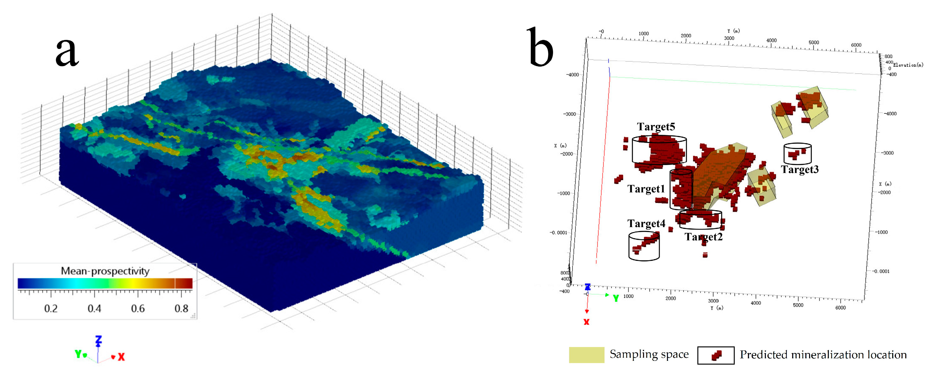
The Figure 9a shows the mean probability deposit prospects for 50 RF models. Based on the prospect map, P–A plot, geological conditions of mineralization, and the results of the benefit–risk analysis, five target areas were identified: Target1, Target2, Target3, Target4, and Target5 (Figure 9b). All five targets are in the high-return–low-risk area. Target1 and Target2 are located to the south and east of the largest known deposit in the center, both at depth on the F7 fault, with a high probability of being large scale and with high potential for mineralization. Target3 is located in the north–central part of F7, within the Xuman Formation, with multiple known gold deposits nearby and Au geochemical anomalies. Target4 is located in the southeast of F5, within the Bianyang Formation, and has Au, As, and Hg geochemical anomalies. Target5 is located in the southern fracture zone area of F1–F7–F17 and has geochemical anomalies at shallow depths. Based on comprehensive analysis, Target1 and Target2 have high prospective potential, followed by Target3, Target4, and Target5 that have low potential.

The RF method was used to model the mineralization probability in the study area. The problem of sample imbalance was solved by using the BLSMOTE method. A total of 50 resampled sets reduced the uncertainty of randomly selecting negative samples and synthesizing positive samples, and quantified the uncertainty using a return–risk analysis. The known deposit is consistent with the high probability zone predicted by the model.

The distribution of predicted results indicates that the position of the ore body is greatly controlled by faults (Figure 10). Known deposits and delineated target areas are closely related to faults. The north–south trending faults, mainly regional faults of F7, constitute the structural system of the study area. The strike of the fault controls the strike of the ore body, while the main fault affects the scale of the ore body. The fault provides a pathway for the migration of deep ore-forming materials. Au, As, and Hg geochemical anomalies are direct indicator elements for ore prospecting. Based on the above geological characteristics and the predicted results of the model, it is indicated that there is significant potential for mineral exploration at the intersection of F7 and F3 faults.

In this study, a comprehensive analysis of mineralization probability in the study area was conducted, employing RF modeling techniques with a focus on addressing sample imbalance using the BLSMOTE method. The results revealed key insights into the reliability and performance of the predictive models.

The study began by assessing the impact of sample balance on the RF models. Three distinct sets were considered: the original sets with randomly selected negative samples, the SMOTE and KMeansSMOTE sets with an equal number of positive and negative samples, and the BLSMOTE sets, which combined positive and negative samples to achieve consistency. It was evident from the analysis that the predictive power of models using balanced samples, particularly the BLSMOTE sets, surpassed that of the non-balanced samples. This observation was substantiated by comparing the variance in the G-mean and F-value between the two techniques, with BLSMOTE exhibiting superior stability.

Among the BLSMOTE models, BLSMOTE18 emerged as the most promising model within the BLSMOTE sets. It boasted the highest G-mean and F-value, indicating excellent performance. The sensitivity of 0.92, specificity of 0.88, and an AUC of 0.9288 further underscored its effectiveness. The selection of an optimal threshold value, 0.33, for delineating potential targets in the P–A plot enhanced its practical utility for the return–risk analysis. Notably, this threshold was associated with a target area encompassing 3% of the study area, capturing 97% of known ore bodies. These parameters collectively supported the conclusion that BLSMOTE models performed exceptionally well and generated reliable results.

To address uncertainties stemming from random negative sample selection, the study employed a return–risk analysis model. This model quantified mineralization occurrence probability, non-occurrence probability, and uncertainty, yielding return and risk maps. The scatter chart was divided into four categories, highlighting areas of high return and low risk as prime targets for exploration. Based on the prospect map, geological considerations, and benefit–risk analysis, five target areas (Target1, Target2, Target3, Target4, and Target5) were identified within the high-return–low-risk zone. Target1 and Target2, situated to the south and east of a central known deposit, exhibited substantial potential for large-scale mineralization. Target3, in the north–central part of F7, showed promise due to nearby gold deposits and geochemical anomalies. Target4, located in the southeast of F5, displayed favorable geochemical anomalies. Target5, in the southern fracture zone, exhibited geochemical anomalies at shallow depths. A comprehensive assessment ranked Target1 and Target2 as high-potential prospects, followed by Target3, Target4, and Target5.

The RF method, coupled with BLSMOTE for sample balancing, proved to be an effective tool for modeling mineralization probability. The results underscored the influence of fault systems on ore body distribution, with known deposits and delineated target areas closely correlated with the regional fault network, particularly F7. The strike of these faults controlled the orientation and scale of ore bodies, while also facilitating the migration of ore-forming materials. Geochemical anomalies of Au, As, and Hg served as valuable indicators for prospecting. Based on the geological characteristics and model predictions, the intersection of F7 and F3 faults emerged as a highly prospective area for mineral exploration.

In conclusion, this study not only successfully addressed sample imbalance but also provided valuable insights into mineralization probability and target identification within the study area. The integration of RF modeling and return–risk analysis yielded reliable results, paving the way for informed decision-making in mineral exploration and resource assessment. Furthermore, the study highlighted the critical role of fault systems in controlling ore body distribution, offering a valuable guideline for future exploration efforts in the region.

5. Conclusions

This paper contributes to the MPM by addressing the problems of unbalanced training data and sample uncertainty. A variety of geological, geochemical, and geomorphological 3D grid models are created in the study area. Training sets are divided based on measured geological profiles. BLSMOTE and random sampling can be used to address data imbalance in supervised machine learning data-driven 3DMPM. Models using balanced datasets outperform unbalanced data, and the BLSMOTE algorithm results are more stable than the SMOTE and KMeansSMOTE algorithms. Uncertainty in the training samples was quantified using return–risk analysis. The prospective target areas are important for further mineralization in the study area.