Abstract
Borehole drilling is required if floor heave in underground mines is to be controlled using bolts through the floor. How well the bolt is anchored depends, in part, on the borehole’s quality. A major factor that can reduce borehole quality is the difficulty of discharging rock fragments from a small-diameter borehole drilled at a downward angle. Therefore, a fuller understanding of the sizes of the rock fragments will aid attempts to achieve smooth fragment discharge. In this study, drilling experiments in the laboratory and SEM imaging were carried out to determine the size and shape of the fragments generated when drilling boreholes in three sedimentary rocks typically found in roadway floors. The results show that the size distribution of the rock fragments conformed to the three-parameter generalized extreme value distribution. The mean fragment size increased with rock density and the mean size of the fragments larger than 1.5 mm increased with the rock’s uniaxial compressive strength. The fractal dimension of the cracks in the fragments was lower for high-density rocks and the mean fragment size was larger for rocks whose cracks had a lower fractal dimension. When a drill rod drills through very dense or high-strength rock, the mean size of the fragments will increase and the discharge power should be increased to prevent fragment discharge blockages. This paper may provide a theoretical basis and a data reference for discharge power settings and discharge channel optimization.
1. Introduction
Coal is the main energy source in China. Statistics show that the coal resource within 2000 m of the surface is about 5.9 trillion tons, of which more than half is below 1000 m [1]. Thus, deep coal mining is imperative to ensure that energy is available for China’s continued economic development. At present, many coal mines in China have moved to deep mining. Under the high stresses in these deep mines, the rocks around most of the mine roadways act like “soft rock” from an engineering standpoint, “soft rock” meaning rock that will undergo significant plastic deformation under a load. The roofs and ribs of these roadways can be seriously deformed and floor heaves are common [2,3,4].
Roof bolting technology has developed rapidly since the 1990s and is widely used in China’s coal mines; it has caused a revolution in coal mine roadway support [5,6,7,8]. In recent years, there have been a series of advancements in the roof bolting techniques used in deep coal mine roadways [9,10,11,12]. However, bolting to control floor heave still has room for improvement. Many researchers have studied floor heave mechanics, and most of them have concluded that floor heave is caused by horizontal compressive stresses that bend the floor strata (Figure 1a). The properties of the floor strata are very important to floor stability [13,14,15,16]. Accordingly, some researchers [17,18,19] have attempted to control floor heave using roof bolting equipment and have achieved good results (Figure 1b). However, there are only a few coal mines in China that use the roof bolting approach to control floor heave. The main reason for not using bolts is that most boreholes for bolting in the floor are drilled downward at a steep angle. Rock fragment discharge is an important part of breaking rock, but there are currently no reference data on the size of the rock fragments generated during borehole drilling. A size mismatch between the rock fragments and the discharge channel coupled with insufficient power to force the fragments out of a deep borehole commonly cause serious blockages and make it more difficult to drill holes (Figure 2).
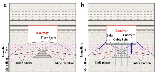
Figure 1.
Sketches showing floor heave and floor heave control with bolts. (a) Floor heave; (b) Floor heave control with bolts and cable bolts.
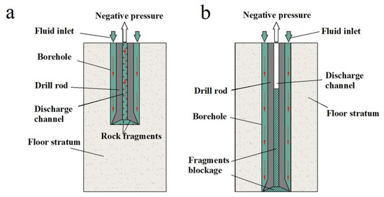
Figure 2.
Diagrams showing discharge channel blockage caused by borehole depth. (a) Fragment discharge from a borehole drilled in a roadway floor; (b) Discharge channel blockage caused by insufficient power to discharge rock fragments owing to great borehole depth.
Brittleness is an intrinsic property of rock. Many studies have been conducted on the size of fragments generated from brittle materials under instantaneous dynamic loads. Grady [20,21] proposed a dynamic fragmentation model by balancing the available kinetic energy against the energy associated with the new surfaces created and derived an equation for mean fragment size. Glenn et al. [22,23] added strain energy to the Grady model and proposed a revised model for mean fragment size based on energy conservation. This model predicted that the strain energy should dominate for brittle materials with low fracture toughness and high fracture-initiation-stress thresholds. Zhou et al. [24] derived expressions for fragment size and strain rate, and calculated the mean fragment size for a wide range of strain rates and a broad range of material properties. Levy and Molinari [25] expanded Zhou’s model further by taking into account defects in the materials. They proposed an equation for calculating the mean fragment size that included material parameters, defect statistics, and the loading rate.
Size distribution is a useful way to describe fragment size. The size distribution of fragments from brittle materials is commonly characterized by the Weibull or Rosin–Rammler distribution [26,27]. Blair [28] analyzed the size distribution of rock fragments produced during blasting and found that the size distribution curve for those rock fragments was similar to a lognormal distribution. Hou et al. [29] and Hogan et al. [30] carried out impact experiments to analyze the fragments from several kinds of brittle rocks and found that the fragment size conformed to the three-parameter generalized extreme value distribution.
The studies mentioned above investigated the characteristics of fragments generated by instantaneous dynamic loads. However, borehole drilling involves imparting a continuous dynamic load to the rock to induce continuous failure. The stresses and energy conversion during fragment generation are obviously different from those generated by instantaneous dynamic loads. Therefore, one cannot expect to obtain accurate size information for drilling fragments using the existing calculation models and distribution functions. In this paper, laboratory experiments were used to analyze the sizes of fragments from three common sedimentary rock types that might be encountered when drilling boreholes in a roadway floor. The results of this work may provide a theoretical basis and reference data for power settings and discharge channel optimization for roadway floor borehole drilling.
2. Laboratory Experiments
2.1. Materials and Methods
Three typical sedimentary coal mine roadway floor rocks were selected as test samples: limestone, gritstone, and mudstone (Figure 3a). The physical and mechanical properties of these specimens are listed in Table 1. A heavy-duty hydraulic automatic drill (Dongguan Zhenjiu Hardware MachineryLTD, Dongguan, China, model CX-15035) was used to drill the boreholes. The drilling rate and rotation rate were set as 0.7 mm/s and 1200 r/min, respectively. A 32 mm-diameter drill bit (Figure 3b) was used for the experiments, the same type of bit used in coal mines. The drilling depth was 20 mm. The drilling fluid (water and rock fragments) generated during drilling was collected in a water tank and piped to a screen with a 0.07 mm mesh size to separate the rock fragments (Figure 3c). The fragments were dried and then categorized as fragments >2.5 mm, 1.5–2.5 mm, 1–1.5 mm, and 0.5–1 mm in size (Figure 3d). Fragments smaller than 0.5 mm, almost all powder, were ignored because they do not significantly affect discharge channel blockages.
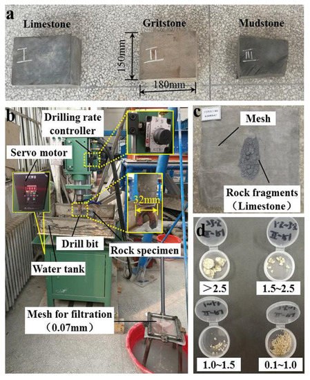
Figure 3.
Photographs of the borehole drilling experiment. (a) Rock specimens; (b) Drilling equipment and rock fragment collection apparatus; (c) Dried limestone rock fragments; (d) Gritstone rock fragments after sieving.

Table 1.
Physical and mechanical properties of the limestone, gritstone, and mudstone rock specimens.
To obtain more accurate data on fragment sizes, the fragments were poured onto a 50 mm × 50 mm sheet of paper (white paper for limestone and mudstone fragments, and black paper for gritstone). The fragments were agitated to make them separate from each other. A Canon 700D SLR camera (Canon Inc., Beijing, China) equipped with a Canon zoom lens (EF-S 1:3.5–5.6 IS STM) was used to take high-resolution photographs of the fragments. The rock fragments from the drilling experiments were divided into the four particle size groups and one high-resolution photograph was taken of each group. If there were too many fragments in a group to fit in one photograph, the fragments were divided into several sub-groups. Taking gritstone as an example, seven high-resolution photographs were obtained, and four of the photographs are shown in Figure 4.
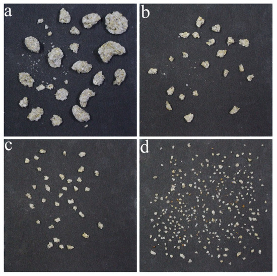
Figure 4.
Four photographs of gritstone fragments showing four different particle sizes. (a) >2.5 mm; (b) 1.5–2.5 mm; (c) 1–1.5 mm; (d) 0.5–1.0 mm.
The photographs were processed with MATLAB software (MathWorks Inc. Natick, MA, USA, ver. 2014b) using the minimum bounding rectangle [31,32]. The horizontal and vertical sizes were determined and the equivalent diameter [33] of each fragment was then calculated. Figure 5 shows the same photographs shown in Figure 4 after image processing.
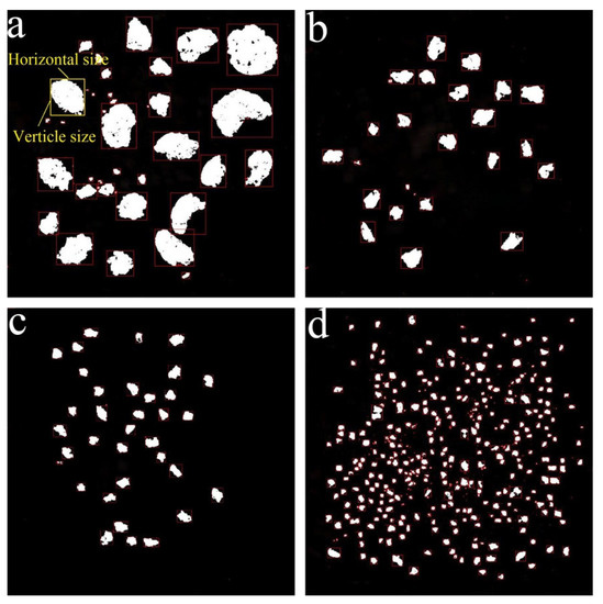
Figure 5.
The same photographs of gritstone fragments shown in Figure 4 after image processing. (a) >2.5 mm; (b) 1.5–2.5 mm; (c) 1–1.5 mm; (d) 0.5–1.0 mm.
2.2. Results and Analysis
2.2.1. Rock Fragment Distribution Curves
Fragment size distributions are commonly analyzed using frequency distribution curves. As the intervals for fragment size on the horizontal axes increase with the number of fragments, the frequency distribution curves plotted with a linear abscissa become very sharp. This has an effect on the analysis of the fragment size distribution. Therefore, in this study, the frequency distribution curves were generated using a log10 transformation of the fragment sizes so that the regularity of the curves could be analyzed more accurately. Rayleigh distributions [25], lognormal distributions [34], Weibull distributions [27], and generalized extreme value distributions [30] are commonly used to analyze the size distribution of fragments generated by instantaneous dynamic loads on brittle materials (glass, rock, etc.). The cumulative frequency distribution functions for the four distributions mentioned above can be represented by Equations (1)–(4).
The Rayleigh distribution is as follows:
where a denotes the scale parameter and x ≥ 0.
The lognormal distribution is as follows:
where denotes the cumulative frequency distribution function of a standard normal distribution, and m and n denote the mean value and standard deviation of a normal distribution, respectively.
The Weibull distribution is as follows:
where k and denote the shape and the scale parameters, respectively, x ≥ 0.
The generalized extreme value distribution is as follows:
where is the shape parameter, is the scale parameter, is the location parameter, and all parameters must satisfy the expression .
As mentioned previously, borehole drilling can be viewed as the continuous failure of rock under a continuous dynamic load. For this reason, maximum likelihood estimation was used to fit the cumulative frequency distribution curves for the equivalent diameter, the horizontal size, and the vertical size of the rock fragments to each distribution function. The results for gritstone are shown in Figure 6.
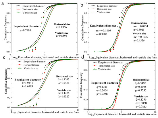
Figure 6.
Cumulative frequency distribution curve fitting results for the equivalent diameter, horizontal size, and vertical size of gritstone drilling fragments. (a) Rayleigh distribution; (b) Lognormal distribution; (c) Weibull distribution; (d) Generalized extreme value distribution.
As can be seen in Figure 6, the Rayleigh distribution function fit (Figure 6a) with a single parameter was significantly worse than the fits to the other three distribution functions. Further, as a two-parameter distribution function, the fit of the lognormal distribution function in Figure 6b was obviously better than that of the Weibull distribution function in Figure 6c. Both the lognormal distribution function and the generalized extreme value distribution (Figure 6d) achieved better fits in that they reflected the size distribution of most fragments sizes better. To obtain the best fitting result, the log likelihoods obtained from fitting tests were analyzed. The results of these tests are illustrated in Figure 7.
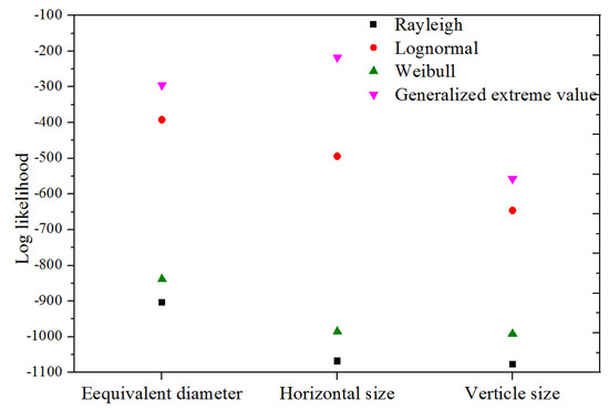
Figure 7.
Log likelihoods obtained from fitting tests on the cumulative frequency distribution curves for the equivalent diameter, horizontal size, and vertical size of gritstone rock fragments.
Figure 7 shows that the log likelihoods of the Rayleigh distribution function with a single parameter were the smallest. The values corresponding to equivalent diameter, horizontal size, and vertical size were −905, −1068, and −1078, respectively, indicating a very poor fit. The log likelihoods of the Weibull distribution were similar to those of the Rayleigh distribution, and the Weibull fit was also poor. In contrast, the log likelihoods of the lognormal distribution function and generalized extreme value distribution function were considerably greater, showing that these two functions fit the data better than the other two functions. The log likelihoods of the generalized extreme value distribution function were −296.263, −217.557, and −557.323, respectively. Apparently, the generalized extreme value distribution function achieved the best fit, so it was the function used to analyze all of the experimental results. The equation for the probability density function is presented as Equation (5) [30].
The expected values can be expressed as the mean size of rock fragments, and these values can be represented by Equation (6):
where , < 1 and ≠ 0.
In many studies, the location parameter has been used as the mean rock fragment size, but as shown in Equation (6), the expected value expressed as the mean rock fragment size is not equal to the location parameter. Therefore, the expected value is a more suitable representation of a rock fragment’s mean size than the location parameter.
2.2.2. Rock Fragment Sizes
The number of rock fragments in each size group for each lithology and their mass, mean equivalent diameter, mean horizontal size, and mean vertical size are listed in Table 2.
Table 2.
Number, particle size, mass, mean equivalent diameter, and mean horizontal and vertical sizes for each size group of limestone, gritstone, and mudstone rock fragments.
As shown in Table 2, there was little difference in the total mass of the rock fragments generated by drilling a 20 mm-deep hole in each of the different rock types. However, the number of fragments generated was quite different. The number of gritstone rock fragments was the largest, followed by mudstone and limestone. The data indicated that the number of fragments increased as the density of the rock decreased; the density of the gritstone was 2415 kg/m3 and that of the limestone was 2678 kg/m3. The denser the rock, the more difficult it was for the particles in the rock to disaggregate. This is consistent with the findings of Hogan [28]. In descending order, the lithologies with the highest number of fragments greater than 1.5 mm in size were mudstone (97 fragments), gritstone (41 fragments), and limestone (16 fragments). By comparing the data in Table 1 and Table 2, it can be seen that the number of large rock fragments increased as the UCS of the rock decreased. As shown in Table 2, the mean fragment size for the three rock types, in descending order, were limestone, mudstone, and gritstone. The mean fragment size was not directly related to rock strength, but it did increase with rock density. This corresponds to the result mentioned above, in that the number of rock fragments increased as the density of the rock decreased and the mean fragment size decreased as the number of fragments increased. To analyze the size distribution of the rock fragments more precisely, the curves fitted by the generalized extreme value distribution function (Equations (4) and (5)) for the cumulative frequency distributions and the percentage composition are presented in Figure 8.
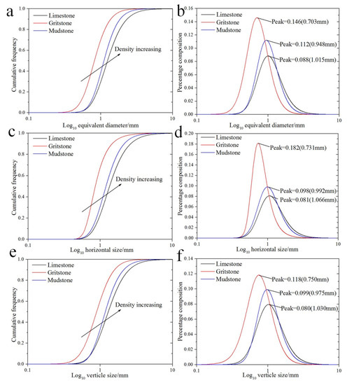
Figure 8.
Fitted cumulative frequency distribution curves and percentage composition curves for the rock fragments from holes drilled in the limestone, gritstone, and mudstone rock specimens. (a) Cumulative frequency distribution curves for equivalent diameter; (b) Percentage composition curve for equivalent diameter; (c) Cumulative frequency distribution curves for horizontal size; (d) Percentage composition curves for horizontal size; (e) Cumulative frequency distribution curves for vertical size; (f) Percentage composition curves for vertical size.
As can be seen in Figure 8a, the gritstone cumulative frequency reached unity first, followed by mudstone and then limestone as the rock densities increased. This demonstrates that the mean equivalent diameter of the fragments generated from gritstone was smallest and the mean equivalent diameter of the fragments generated from limestone was the largest. The results indicated that the mean equivalent diameter of the rock fragments increased with density. The percentage composition curves for equivalent diameters are shown in Figure 8b. There were some differences between the rock fragment peak values. The peak values for the equivalent diameters were, in descending order, 1.015 mm (limestone), 0.948 mm (mudstone), and 0.703 mm (gritstone). It can be seen that the equivalent diameters of the fragments accounting for the largest percentage of the three lithologies increased with rock densities. The frequency distribution curve for gritstone was the narrowest, indicating that the range of equivalent diameters for gritstone fragments was smaller than the ranges for the fragments from the other two lithologies. In contrast, the percentage composition curve for limestone was the widest, indicating that the equivalent diameters covered a wider range. These features will be discussed in more detail later. The cumulative frequency distribution curves for horizontal size are shown in Figure 8c. Like the equivalent diameter curves, the mean horizontal size curves for the rock fragments were, in descending order, limestone, mudstone, and gritstone. The result shows that the mean horizontal size of rock fragments increased as the rock density increased. The percentage composition curves for horizontal size in Figure 8d show that the horizontal size peak values were similar to the equivalent diameter peak values in that the limestone horizontal size of the fragments accounting for the largest percentage was the highest (1.066 mm) and that of gritstone was the lowest (0.731 mm). The cumulative frequency distribution curves for vertical size are presented in Figure 8e. The mean vertical sizes of the rock fragments in descending order were limestone, mudstone, and gritstone; the sizes increased with rock density. The percentage composition curves for vertical size are shown in Figure 8f. The horizontal size of the limestone fragments was the largest (1.030 mm) and they accounted for the highest percentage, whereas the horizontal size of the gritstone fragments, the lowest percentage, was the smallest (0.750 mm). All the above data indicate that the mean size of the rock fragments generated during drilling was larger when the rock being drilled was denser.
The location and scale parameters, and , are important parameters in the equation that defines the generalized extreme value distribution function, Equation (4). The different and values for the fitted curves are shown in Figure 9.
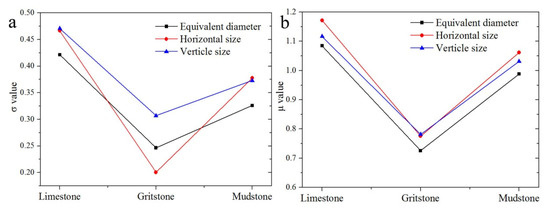
Figure 9.
Location, , and scale, , values for the fitted curves for each rock fragment lithology. (a) values; (b) values.
The scale parameter represents the magnitude of the range in the frequency distribution curves. That is, the value of is higher when the range of fragment sizes is larger. In Figure 9a, the values for the three fragment lithologies, in descending order, are limestone, mudstone, and gritstone. This means that the range of fragment sizes from limestone was the largest and the size range for the gritstone fragments was the smallest. The values determine the position of the percentage composition curves on the horizontal axes; a higher value means that the fragments are larger. In Figure 9b, the values for each lithology, in descending order, were limestone, mudstone, and gritstone. This means that the drilling-generated limestone fragments were larger than the fragments from the other two rock types. The values of and determined the size distribution of the fragments, and these two values increased with rock density. As and increased, the range of rock fragment sizes also increased and this resulted in an increase in the mean size of the rock fragments.
Because the size of the discharge channel is fixed, the generation of large fragments has a considerable influence on fragment discharge when drilling boreholes in the floor. Therefore, analyzing the size of the rock fragments larger than 1.5 mm in diameter is especially important. The fitted curves for the cumulative frequency distribution and percentage composition curves for rock fragments larger than 1.5 mm are shown in Figure 10.
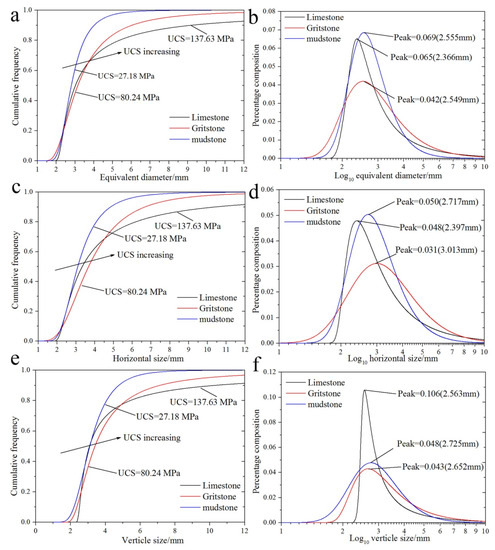
Figure 10.
Fitted cumulative frequency distribution curves and frequency distribution curves for the rock fragments larger than 1.5 mm from holes drilled in the limestone, gritstone, and mudstone. (a) Cumulative frequency distribution curves for equivalent diameter; (b) Percentage composition curves for equivalent diameter; (c) Cumulative frequency distribution curves for horizontal size; (d) Percentage composition curves for horizontal size; (e) Cumulative frequency distribution curves for vertical size; (f) Percentage composition curves for vertical size.
The curves in Figure 10a,c,e show that the cumulative frequency distributions of fragments larger than 1.5 mm are different from the distributions of fragments in the full size range. The cumulative frequency of mudstone reached unity first, followed by gritstone and limestone. This demonstrates that the mean equivalent diameter of the fragments generated from mudstone was the smallest and the mean equivalent diameter of the fragments generated from limestone was the largest. The mean size of the fragments larger than 1.5 mm in descending order was limestone, gritstone, and mudstone. The UCSs for the three rocks are 137.63, 80.24, and 27.18 MPa, which means that the mean size of rock fragments increased with the UCS of the rocks. From Figure 10b,d,f, it can be observed that there was no systematic variation in the peak values for the frequency distribution curves. The sizes corresponding to the peak values were all roughly in the 2.5–3.0 mm range but the curve shapes were quite different. To summarize, the mean size of fragments larger than 1.5 mm increased as the rock UCS increased.
3. Scanning Electron Microscopy
3.1. Fracture Surface Morphologies
An FEI Quanta 250 FEG Field Emission Scanning Electron Microscope (FEI, Hillsboro, OR, USA) (Figure 11a) was used to take secondary electron (SE) images of the fragments’ surfaces to explore the relationship between crack development and fragment shape. The composition of the mineral phases was determined by energy-dispersive X-ray spectroscopy. Selected fragments, gold-coated for SE imaging, are shown in Figure 11b.
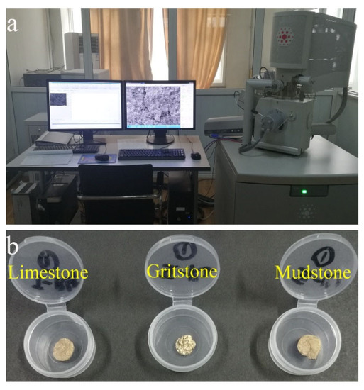
Figure 11.
Photographs of (a) An FEI Quanta 250 FEG Field Emission Scanning Electron Microscope; (b) Selected gold-coated rock fragments prepared for secondary electron imaging.
Secondary electron images of limestone fragments are shown in Figure 12. It can be seen that the surfaces of the limestone fragments were inlaid with clustered or granular masses of calcite (Figure 12a,b). The surfaces of the fragments were relatively rough with many scaly cracks. These cracks did not penetrate the fragments, but were oriented parallel to the surface. The cracks were generally relatively long and are commonly more than 500 µm in length. If the fragment was broken again along these cracks by a cutting force, the cracks would expand and additional small fragments would be generated. As shown in Figure 12b, one calcite block was 860 µm long and 572 µm wide. From Figure 12c, at a magnification of 1600×, it can be seen that there were several lamellar structures on the limestone fragment’s surface and the cracks developed parallel to the surface. These cracks could cause small lamellar fragments to form.
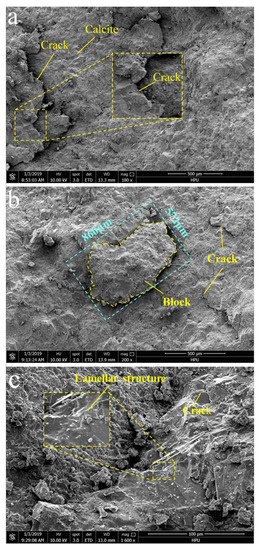
Figure 12.
Secondary electron SEM images of limestone fragments. (a) Cracks developed parallel to the surface; (b) Block on the surface; (c) Lamellar structure.
Microscopic SE images of gritstone fragments are shown in Figure 13. The gritstone fragment surfaces were not as flat and solid looking as the limestone fragment surfaces. There were many cracks and pores on the gritstone surfaces and there were many small mica grains protruding. The cracks, generally open, were commonly perpendicular to the surface and penetrated the fragments. Figure 13c shows a Y-shaped crack formed by the intersection of two cracks. The maximum and minimum distances across this open Y-shaped crack were 94.5 µm and 36.8 µm. The numerous cracks and loose structure suggest that the gritstone fragments would readily break apart to form smaller spherical fragments if they were subjected to a cutting force.
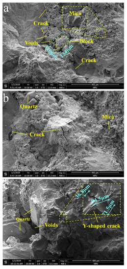
Figure 13.
Secondary electron SEM images of gritstone fragments. (a) Cracks penetrating a fragment; (b) Quartz and mica; (c) Y-shaped crack.
Figure 14 shows SE images of mudstone fragments. As shown in Figure 14a,b, the surfaces of mudstone fragments were relatively smooth and compact (note that the long dimension of the field of view in Figure 14b was ~35 µm). There were numerous kaolinite grains adhering to the surface and there were few pores. The crack orientation was similar to the cracks in the limestone. A few of the cracks were parallel to the surfaces, but most of them penetrated the fragment. The openings across the cracks were generally small and the gap was commonly 50 µm or less. Figure 14c shows a 166 µm by 141 µm block on the surface of a mudstone fragment bounded by two cracks. This kind of cracking may have been the reason that mudstone fragments were not lamellar, like the limestone fragments, or spherical, like the gritstone fragments. The mudstone fragments were polyhedrons with distinct edges and angles.
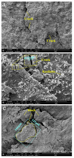
Figure 14.
Secondary electron SEM images of mudstone fragments. (a) Cracks developed parallel to the surface; (b) Cracks penetrating a fragment; (c) Block on a mudstone fragment’s surface.
3.2. Fractal Dimension of Cracks in Fragments
To quantify the characteristics of the cracks observed on the fragments’ surfaces, the fractal dimensions of the cracks in the SEM images were calculated. The fractal dimension reflects a crack’s complexity. A higher fractal dimension means that the crack can be broken more easily by a cutting force and thus further failure is more likely to occur [35,36]. A box-counting algorithm is one of the most common methods used to calculate the fractal dimension of two-dimensional spaces. An equation for determining the fractal dimension of fractures is presented below as Equation (7) [37]:
where ε denotes the size of a square box, ε = ε0, ε1,…εi, i = 0,1,2,3···; denotes the number of the square boxes; A is a constant; and D denotes the fractal dimension.
Taking the logarithm of both sides of Equation (7) yields:
As shown in Equation (8), the transformed fractal dimension D can be represented by the slope of the −(−) curve.
A digital image is composed of an array of pixels. A binary image is only composed of black and white pixels; therefore, it has high discreteness and any target area in a binary image is easy to recognize [38]. Therefore, the cracks in the SEM images (Figure 12, Figure 13 and Figure 14) can be easily extracted and binarized using MATLAB software by adjusting the gray value of the image. Thirteen binarized images of representative cracks in the rock fragments are shown in Figure 15.
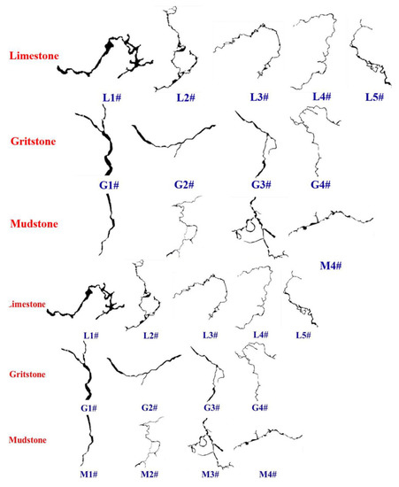
Figure 15.
Binarized images of representative cracks in the limestone, gritstone, and mudstone rock fragments.
The Fraclab subroutine in MATLAB was used to calculate the box-counted dimension of the cracks to obtain the values for and . Then, the least squares fitting method was used to define the −(−) curves shown in Figure 16.
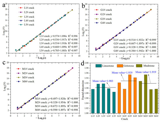
Figure 16.
Log2(N)-(−Log2(ε)) curves for rock fragment cracks and a bar chart summarizing the crack fractal dimensions. (a) Limestone; (b) Gritstone; (c) Mudstone; (d) bar chart summarizing the fractal dimensions of the cracks.
The correlation coefficients for the fitted lines in Figure 16 were all greater than 0.99. The fractal dimensions for the cracks in rock fragments of the same lithology were almost the same; the curves in each panel in Figure 16 are almost coincident. In Figure 16a, the fractal dimensions of cracks L1#–L5# are 1.896, 1.917, 1.918, 1.899, and 1.885, respectively. Figure 16b shows that the fractal dimensions of the gritstone cracks are significantly higher than the limestone cracks’ fractal dimensions; the values for the G1#–G4# cracks are 1.922, 1.897, 1.954, and 1.942, respectively. In Figure 16c the fractal dimensions of the mudstone cracks, M1#–M5#, are 1.928, 1.954, 1.895, and 1.879, respectively. As shown in Figure 16d, the mean fractal dimensions for the cracks in the three rock types are gritstone 1.929, mudstone 1.919, and limestone 1.903. This suggests that the fractal dimensions of cracks in the fragments increased as the rock density decreased. The fractal dimension of these two-dimensional cracks was between one and two. The fractal dimension of the gritstone cracks was the largest; thus, the crack development degree was the highest. Further failure would occur if the crack developed more and the resulting fragments would be smaller in size. Therefore, gritstone generated the most fragments and the mean fragment size was the smallest. Similarly, the cracks in limestone fragments had the smallest fractal dimension and the mean fragment size was the largest. The results of this fractal analysis are consistent with the results of the drilling experiments described in Section 2.
4. Discussion
This paper reports on the results of laboratory drilling experiments carried out to analyze the size of rock fragments generated when drilling boreholes in mine roadway floors. Cumulative frequency curves of the experimental results showed that the equivalent diameter, horizontal size, and vertical size of the rock fragments produced conformed to the three-parameter generalized extreme value distribution model. Analysis of the curves’ fits to the model demonstrated that the mean fragment size increased with rock density. The scale parameter and location parameter determined the distribution of fragment sizes, and both of them increased with rock density. When and increased, the range of rock fragment sizes also increased, and this resulted in an increase in the mean size of the rock fragments. A statistical analysis of the rock fragments larger than 1.5 mm suggested that the mean size increased as the rock’s UCS increased.
The SEM images show that some of the cracks in the limestone fragments developed parallel to the fragment’s surface. If the fragments were subjected to a cutting force, the cracks could expand to generate smaller, lamellar fragments. Most of the cracks in gritstone developed perpendicular to the surface and many of these cracks were open and relatively wide. This means that the gritstone fragments were easily broken, and when broken, they could generate many small secondary spherical fragments. The cracks in the mudstone fragments were both parallel and perpendicular to the surface and when the mudstone fragments were broken along these cracks, new polyhedral fragments with distinct edges and angles were produced. The fractal dimensions determined by the box-counting method were lower for rocks with higher densities and the mean fragment size was larger when the fractal dimension is lower.
To summarize, the size of the rock fragments generated when drilling boreholes in mine roadway floors is closely related to the density and UCS of the rock, as well as to crack complexity, as illustrated in Figure 17.
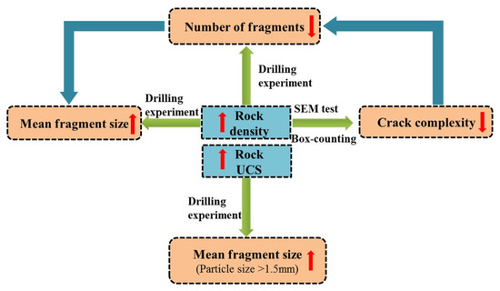
Figure 17.
Relationships between fragment size, rock density, uniaxial compressive strength, and crack complexity.
5. Conclusions
The sizes of rock fragments have an important influence on fragment discharge when drilling boreholes in roadway floors. Laboratory drilling experiments and SEM investigations were conducted to explore the size and shape of drilling fragments generated from three sedimentary rocks typically found in roadways. A box-counting algorithm was used to analyze the fractal dimensions of the cracks in SEM images of the rock fragments. The following conclusions were drawn.
The size distribution of the rock fragments generated during drilling conformed to the three-parameter generalized extreme value distribution. Both the scale parameter and location parameter increased with rock density. The mean fragment size also increased with rock density and the mean size of fragments larger than 1.5 mm increased with the rock’s uniaxial compressive strength.
There was a relationship between crack orientations and the fragment’s lithology and shape. For example, cracks in limestone fragments were, in most cases, parallel to the fragment’s surface and the fragments were most commonly lamellar in shape. The fractal dimension of cracks was lower for cracks that occurred in rocks of higher density. The mean fragment size was larger for lithologies whose cracks had a lower fractal dimension.
During borehole drilling in the roadway floor, the discharge power should be adjusted according to the physical and mechanical properties of the floor strata. When the drill rod drills through very dense or high-strength rock, the mean size of the fragments will increase and the discharge power should be increased to prevent fragment discharge blockages. The results presented in this paper may provide a theoretical basis and a data reference for discharge power settings and discharge channel optimization that should improve roadway floor bolt hole drilling results.
Author Contributions
Conceptualization, M.F.; Data curation, S.H.; Formal analysis, M.F. and S.H.; Funding acquisition, M.F. and S.L.; Investigation, M.F. and S.H.; Methodology, M.F. and S.L.; Resources, H.J.; Supervision, M.F.; Validation, S.H. and H.J.; Writing—original draft, S.H.; Writing—review and editing, M.F. All authors have read and agreed to the published version of the manuscript.
Funding
This work was funded by the National Natural Science Foundation of China (grants 52104083 and 52074102), the Open Research Fund of the State Key Laboratory of Coal Resources and Safe Mining, CUMT (SKLCRSM22KF007), the Key R & D and promotion projects in Henan Province (222102320169), and the Key Scientific Research Projects of Colleges and Universities in Henan Province (22A440004).
Data Availability Statement
The data used to support the findings of this study are available from the corresponding author upon request.
Acknowledgments
Thanks to the relevant departments for fundings.
Conflicts of Interest
The authors declare no conflict of interest.
References
- Kang, H.P.; Wang, G.F.; Jang, P.F.; Wang, J.C.; Zhang, N.; Jing, H.W.; Hang, B.X.; Yang, B.G.; Guan, X.M.; Wang, Z.G. Conception for strata control and intelligent mining technology in deep coal mines with depth more than 1000 m. J. China Coal Soc. 2018, 43, 1789–1800. [Google Scholar]
- Jiao, Y.Y.; Song, L.; Wang, X.Z.; Adoko, A.C. Improvement of the U-shaped steel sets for supporting the roadways in loose thick coal seam. Int. J. Rock Mech. Min. Sci. 2013, 60, 19–25. [Google Scholar] [CrossRef]
- Liu, Q.S.; Kang, Y.S.; Bai, Y.Q. Research on supporting method for deep rock roadway with broken and soft surrounding rock in Guqiao Coal Mine. Rock Soil Mech. 2011, 32, 3097–3104. [Google Scholar]
- Kang, Y.S.; Liu, Q.S.; Xi, H.L. Numerical analysis of THM coupling of a deeply buried roadway passing through composite strata and dense faults in a coal mine. Bull. Eng. Geol. Environ. 2014, 73, 77–86. [Google Scholar] [CrossRef]
- Ma, N.J.; Hou, C.J. Theories and Applications of the Ground Pressure in Coal Mine Roadways; China Coal Industry Publishing House: Beijing, China, 1995. [Google Scholar]
- Peng, S. Topical areas of research needs in ground control: A state of the art review on coal mine ground control. Int. J. Min. Sci. Technol. 2010, 25, 1–6. [Google Scholar] [CrossRef]
- Murphy, M.; Finfinger, G.L.; Peng, S. Guest editorial—Special issue on ground control in mining. Int. J. Min. Sci. Technol. 2016, 26, 1–2. [Google Scholar] [CrossRef]
- Kang, H.P. Analysis on the application of bolt support in coal mine roadways. China J. Rock Mech. Eng. 2010, 29, 649–664. [Google Scholar]
- Basarir, H.K.; Sun, Y.T.; Li, G.C. Gateway stability analysis by global-local modeling approach. Int. J. Rock Mech. Min. Sci. 2019, 113, 31–40. [Google Scholar] [CrossRef]
- Zhang, W.; He, Z.M.; Zhang, D.S.; Qi, D.H.; Zhang, W.S. Surrounding rock deformation control of asymmetrical roadway in deep three-soft coal seam: A case study. J. Geophys. Eng. 2018, 15, 1917–1928. [Google Scholar] [CrossRef]
- Huang, W.P.; Yuan, Q.; Tan, Y.L.; Wang, J.; Liu, G.L.; Qu, G.L.; Li, C. An innovative support technology employing a concrete-filled steel tubular structure for a 1000-m-deeproadway in a high in situ stress field. Tunn. Undergr. Space Technol. 2018, 73, 26–36. [Google Scholar] [CrossRef]
- Jia, H.S.; Wang, L.Y.; Liu, S.W.; Feng, Z.Y.; Fu, M.X. Design of multi-layer coupling support and span of setup entry roof at depth. Arab. J. Geosci. 2018, 11, 488–498. [Google Scholar] [CrossRef]
- Yang, J.H.; Song, G.F.; Yang, Y.; Yang, Z.Q. Application of the complex variable function method in solving the floor heave problem of a coal mine entry. Arab. J. Geosci. 2018, 11, 515–529. [Google Scholar] [CrossRef]
- Sun, X.M.; Chen, F.; He, M.C.; Gong, W.L.; Xu, H.C.; Lu, H. Physical modeling of floor heave for the deep-buried roadway excavated in ten degree inclined strata using infrared thermal imaging technology. Tunn. Undergr. Space Technol. 2017, 63, 228–243. [Google Scholar] [CrossRef]
- Chang, Q.L.; Zhou, H.Q.; Xie, Z.H.; Shen, S.P. Anchoring mechanism and application of hydraulic expansion bolts used in soft rock roadway floor heave control. Int. J. Min. Sci. Technol. 2013, 23, 323–328. [Google Scholar] [CrossRef]
- Tang, S.B.; Tang, C.A. Numerical studies on tunnel floor heave in swelling ground under humid conditions. Int. J. Rock Mech. Min. Sci. 2012, 55, 139–150. [Google Scholar] [CrossRef]
- Wang, C.L.; Li, G.Y.; Gao, A.S.; Shi, F.; Lu, Z.J.; Lu, H. Optimal pre-conditioning and support designs of floor heave in deep roadways. Geomech. Eng. 2018, 14, 429–437. [Google Scholar]
- Kang, Y.S.; Liu, Q.S.; Gong, G.Q.; Wang, H.C. Application of a combined support system to the weak floor reinforcement in deep underground coal mine. Int. J. Rock Mech. Min. Sci. 2017, 71, 143–150. [Google Scholar] [CrossRef]
- Liu, S.W.; Zhang, W.G.; Feng, Y.L. Study on migration mechanism of slipping floor heave rock mass in deep roadway and its control countermeasure. J. Min. Saf. Eng. 2013, 30, 706–711. [Google Scholar]
- Grady, D.E. Local inertial effects in dynamic fragmentation. J. Appl. Phys. 1982, 53, 322–325. [Google Scholar] [CrossRef]
- Grady, D.E. Fragment size prediction in dynamic fragmentation. AIP Conf. Proc. 1982, 78, 456–459. [Google Scholar]
- Glenn, L.A.; Gommerstadt, B.Y.; Chudnovsky, A. A fracture mechanics model of fragmentation. J. Appl. Phys. 1986, 60, 1224–1226. [Google Scholar] [CrossRef]
- Glenn, L.A.; Chudnovsky, A. Strain energy effects on dynamic fragmentation. J. Appl. Phys. 1986, 59, 1379–1380. [Google Scholar] [CrossRef]
- Zhou, F.H.; Molinari, J.F.; Ramesh, K.T. Effects of material properties on the fragmentation of brittle materials. Int. J. Fract. 2006, 139, 169–196. [Google Scholar] [CrossRef]
- Levy, S.; Molinari, J.F. Dynamic fragmentation of ceramics, signature of defects and scaling of fragment sizes. J. Mech. Phys. 2010, 58, 12–26. [Google Scholar] [CrossRef]
- Weibull, W. A statistical theory of the strength of materials. Ing. Kapsakad. Handl. 1939, 151, 1–45. [Google Scholar]
- Cheong, Y.S.; Reynolds, G.K.; Salman, A.D.; Hounslow, M.J. Modelling fragment size distribution using two-parameter Weibull equation. Int. J. Miner. Process. 2004, 74, S227–S237. [Google Scholar] [CrossRef]
- Blair, D.P. Curve-fitting schemes for fragmentation data. Fragblast 2004, 8, 137–150. [Google Scholar] [CrossRef]
- Hou, T.X.; Xu, Q.; Yang, X.G.; Lu, P.Y.; Zhou, J.W. Experimental study of the fragmentation characteristics of brittle rocks by the effect of a free fall round hammer. Int. J. Fract. 2015, 194, 169–185. [Google Scholar] [CrossRef]
- James, D.H.; Robert, J.R.; John, G.S.; Suporn, B. Dynamic fragmentation of granite for impact energies of 6–28 J. Eng. Fract. Mech. 2012, 79, 103–125. [Google Scholar]
- Yuan, K.F.; Tao, D.C.; Xu, H.; Xie, W. Pepper grading based on the minimum bounding rectangle. Chin. Agric. Sci. Bull. 2016, 32, 166–170. [Google Scholar]
- Zhou, J.X. MATLAB from Entry to Mastery; Posts and Telecommunications Press: Beijing, China, 2008; pp. 235–254. [Google Scholar]
- Salman, A.D.; Fu, J.; Gorham, D.A.; Hounslow, M.J. Impact breakage of fertiliser granules. Powder Technol. 2003, 130, 359–366. [Google Scholar] [CrossRef]
- Wang, H.; Ramesh, K.T. Dynamic strength and fragmentation of hot-pressed silicon carbide under uniaxial compression. Acta Mater. 2004, 52, 355–367. [Google Scholar] [CrossRef]
- Cai, J.C.; Wei, W.; Hu, X.Y.; Liu, R.C.; Wang, J.J. Fractal characterization of fracture network extension in porous media. Fractals 2017, 23, 1750023. [Google Scholar] [CrossRef]
- Xie, H.P.; Gao, F.; Zhou, H.W.; Zuo, J.P. Study on the fractal characteristics of rock fracture and broken. J. Disaster Prev. Mitig. Eng. 2003, 123, 1–9. [Google Scholar]
- Dreuzy, J.R.D.; Davy, P.; Bour, O. Hydraulic properties of two-dimensional random fracture networks following a power law length distribution: 1. Effective connectivity. Water Resour. Res. 2001, 37, 2065–2078. [Google Scholar] [CrossRef]
- Peng, R.D.; Xie, H.P.; Ju, Y. Computation method of fractal dimension for 2-D digital image. J. China Univ. Min. Technol. 2004, 33, 20–24. [Google Scholar]


Disclaimer/Publisher’s Note: The statements, opinions and data contained in all publications are solely those of the individual author(s) and contributor(s) and not of MDPI and/or the editor(s). MDPI and/or the editor(s) disclaim responsibility for any injury to people or property resulting from any ideas, methods, instructions or products referred to in the content. |
© 2023 by the authors. Licensee MDPI, Basel, Switzerland. This article is an open access article distributed under the terms and conditions of the Creative Commons Attribution (CC BY) license (https://creativecommons.org/licenses/by/4.0/).