4.1. Method Ⅰ
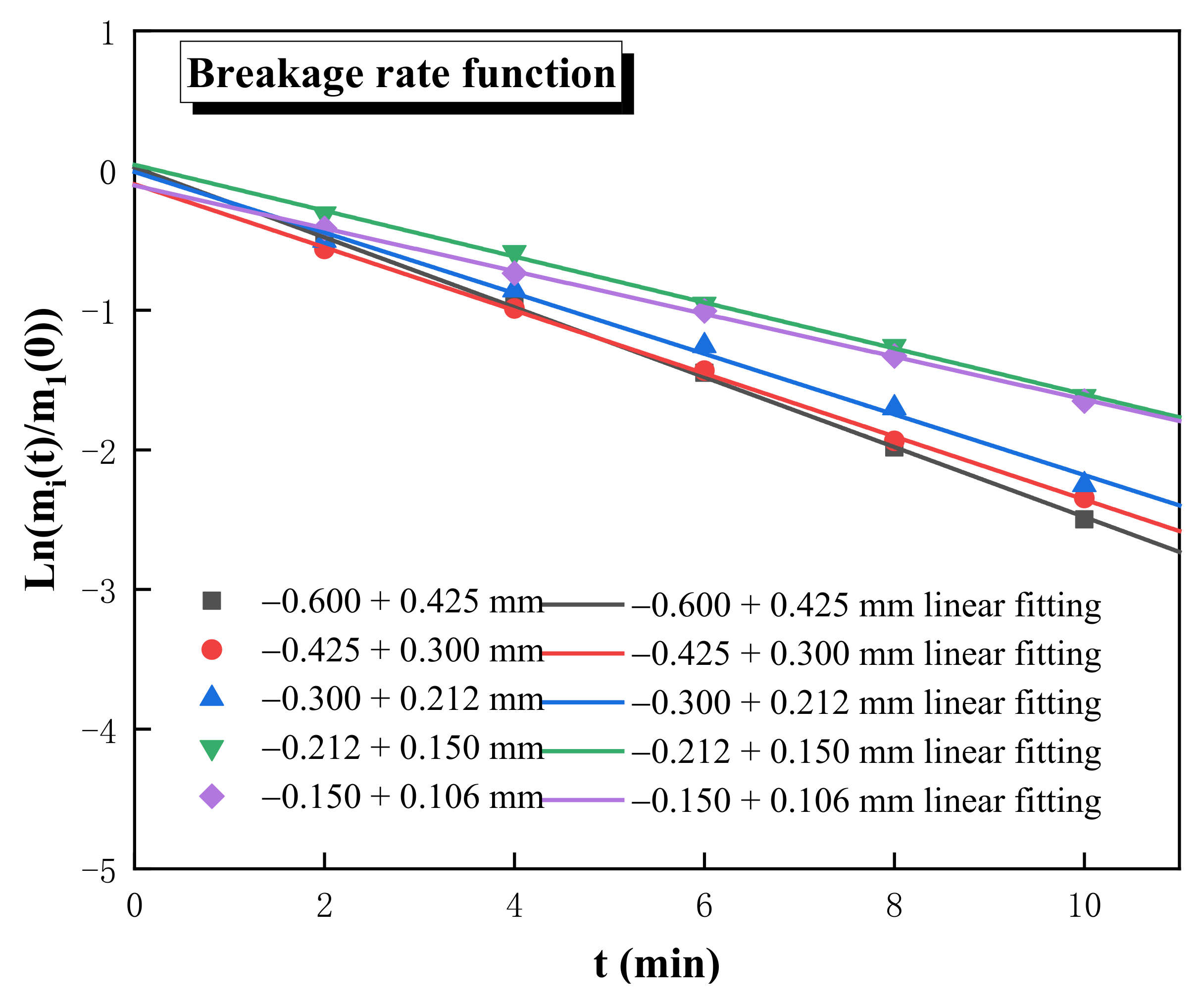
The test results obtained from Equation (6) are shown in
Figure 3. In the range of the feed fractions, magnetite met the first-order linear grinding kinetics, and the slope of the straight line was the breakage rate function of magnetite in this feed fraction.
Table 3 shows the linear fitting equation for each fraction and its linear correlation. As can be seen, the value of the breakage rate function dropped from 0.25 min
−1 to 0.15 min
−1 as the particle size decreased. The reason for this phenomenon is that the compressive strength of mineral particles increased as the particle size decreased, which directly caused difficulty in grinding the mineral, also known as the size effect of the particle. Theoretically, the fitted curves of each fraction should pass through the origin of the coordinate axes; however, the fitted curves of the five feed fractions in this test all had vertical intercepts, and the sieving error was the main reason for this problem. Nevertheless, this can be introduced into the breakage parameter correction and has no influence on the calculation of the breakage rate function.
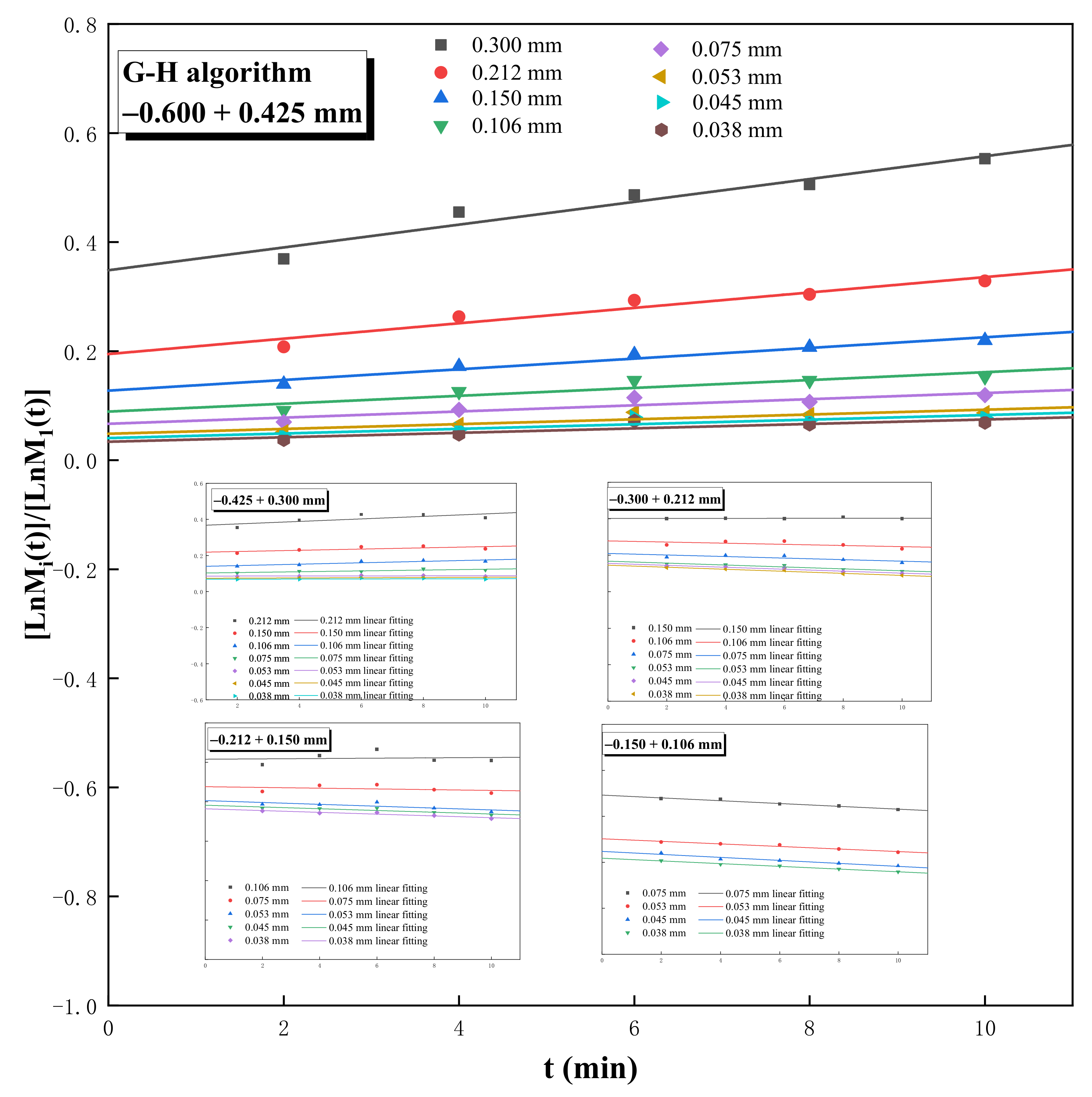
In this study, the G–H and BⅡ algorithms were used to calculate the values of the cumulative breakage distribution function Bi1. When the grinding kinetic model is a first-order linear type, in the G–H algorithm, [lnMi(t)]/[lnM1(t)] is a function of grinding time t, and Bi1 is the vertical coordinate intercept when t = 0.
Figure 4 shows the result of the G–H algorithm. For a feed fraction of −0.600 + 0.425 mm, the value of B
i1 was between 0 and 0.4, and the smaller the particle size, the finer the value of B
i1 was. Furthermore, because the breakage characteristic was abrasion, it was outstandingly characterized by a low yield of intermediate daughter fractions, resulting in a more convergent value of B
i1 within a certain particle size range. Generally, as the feed fraction becomes finer, the decrease in the number of daughter fractions leads to an increase in the B
i1 value of each daughter fraction.
When using the BⅡ algorithm to calculate the cumulative breakage distribution function, a relatively short grinding time was chosen, and the appropriate grinding time was generally no more than 65% of the breakage rate of the feed fractions. When the grinding time of the magnetite ore was 2 min, only 45.75% of −0.600 + 0.425 mm magnetite was crushed, which was in line with the range of the BⅡ algorithm.
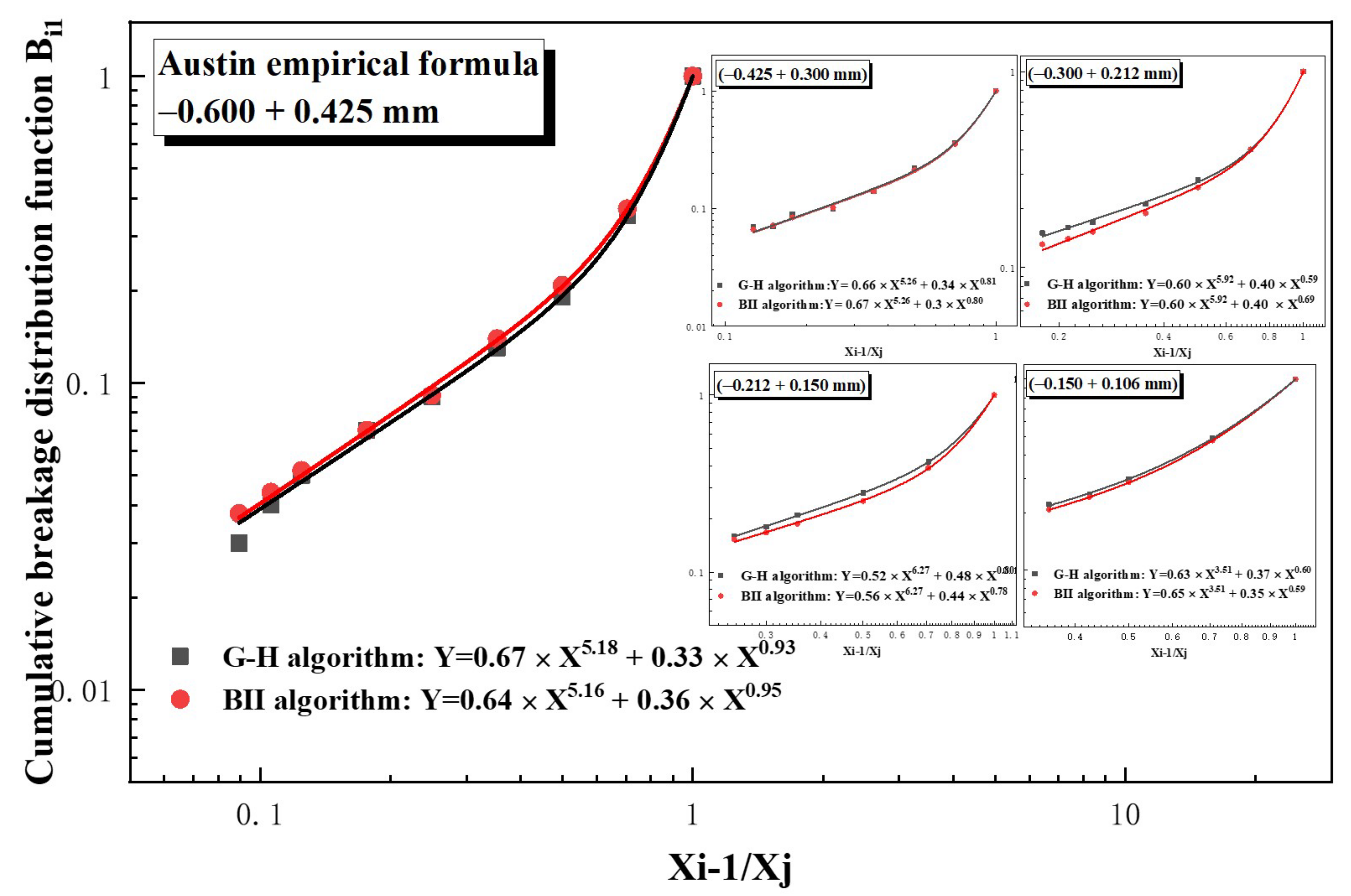
The calculation results of the two algorithms were brought into the Austin empirical formula, and the fitting results are shown in
Figure 5. The curves fitted using the two methods were relatively similar, and the values of the fragmentation parameters φ, γ, and β for the magnetite produced with the fit are summarized in
Table 4 for a better comparison of the two algorithms. The parameter values obtained using the two methods showed very little variation and were within the error of the calculation results. Taking the −0.600 + 0.425 mm grain size as an example, the maximum calculation error was only 0.03, and hence it can be concluded that the calculation of B
i1 was relatively accurate. However, when it came to the finest feed fraction −0.150 + 0.106 mm, the fitting results were far from the results of other coarser feed fractions. One possible reason for the difference is that fewer data points were used for fitting, resulting in larger fitting errors, and another possible reason is that it was more difficult to determine the endpoint of sieving in the finer fractions, leaving a larger experimental error. It was critical to have sufficient data points in the fit, and the number of data points should preferably be more than five.
γ is a parameter indicating the magnitude of the mechanical strength. As the feed size decreased, the γ value gradually increased, which was another manifestation of the size effect of the particles.
4.2. Method Ⅱ
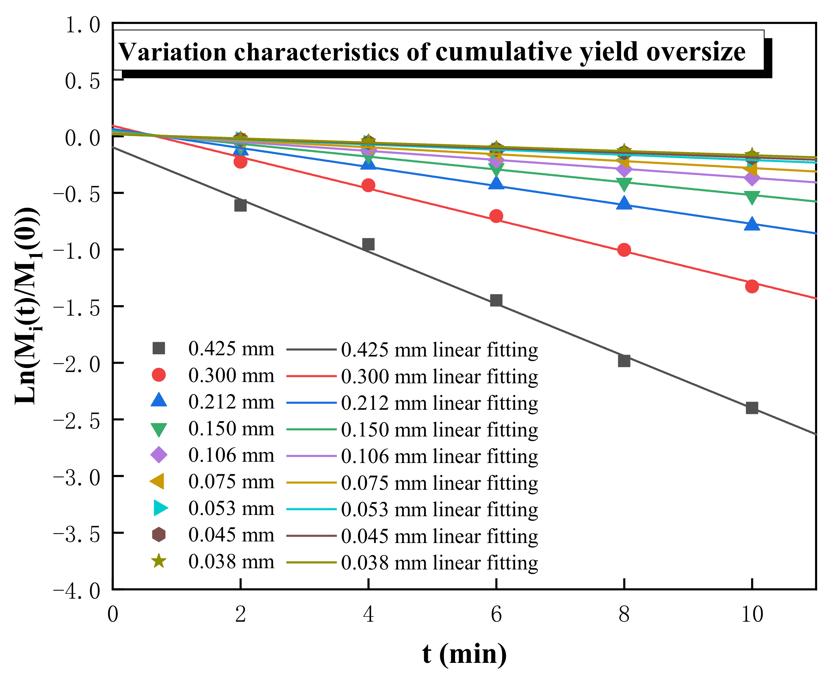
It was found that the variation in t would not affect the change rate of the cumulative mass fraction coarser than size class i at time t; M
i(t) also followed the first-order grinding kinetics. Taking −0.600 + 0.425 mm as an example,
Figure 6 shows that ln[M
i(t)]/M
1(0)] changed in characteristics after grinding time t, suggesting a high linear fit correlation between ln[M
i(t)]/M
1(0)] and t. Additionally, the fitting equation and linear fit correlation coefficient R
2 are shown in
Table 5. The R
2 of the last two size classes decreased because of their lower yields, the fitting results of which would be greatly affected by experimental chance errors. The
value gradually decreased as the particle size became finer, indicating that the generation rate of the fine particle size was significantly lower than that of the coarse particle size.
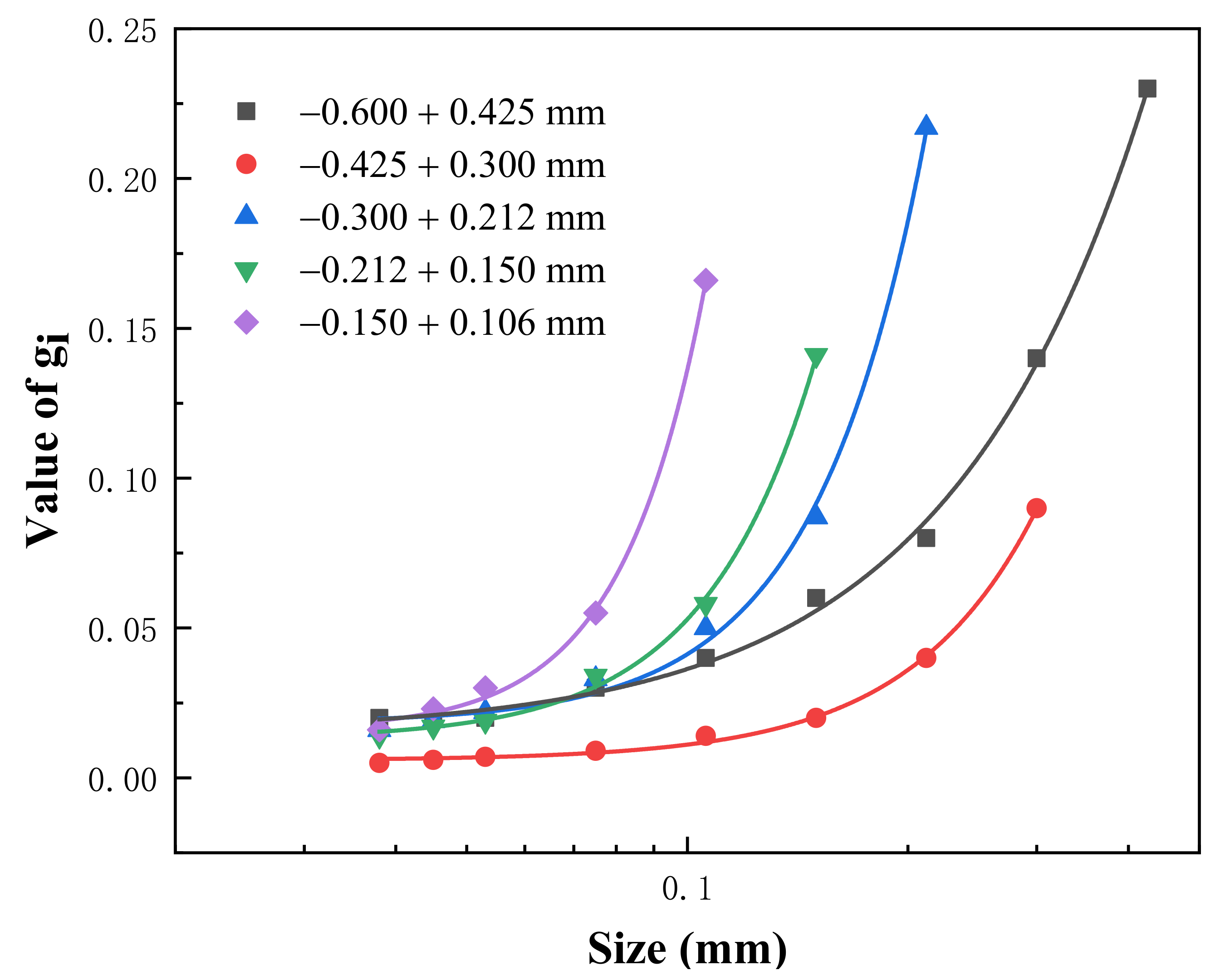
Figure 7 shows the variation in the
gi value with different particle sizes. Additionally, taking the value of −0.600 + 0.425 mm as an example, the values of k
0, k
1, and a were 0.007, 0.786, and 1.666, respectively, by fitting the
gi function, and the R
2 value was 0.9978. The parameters calculated with regression were plugged into Equation (15):
Since k
0 is a parameter for the experimental chance error, when its value tends to be 0, it can be neglected, so Equation (20) can be abbreviated as follows:
The final grinding kinetic model calculated using Method Ⅱ was obtained by combining Equations (18) and (21):
The remaining four feed fractions were calculated according to the above method, and the values of the calculated parameters k
1, k
2, and a are shown in
Table 6.
4.3. Simulation and Comparison
While processing the grinding of magnetite, the breakage rate function S
1 can be determined using Equation (6), the cumulative breakage distribution function B
i1 can be generated using Equation (9), and the rate constant
gi can be calculated using Equation (15). These parameters were input into Equations (10) and (18) for simulation, and the models derived from the two methods for each of the feed fractions are shown in
Table 7 (when i = 1, the two methods yield the same model, so they are not listed). Because Method Ⅱ involves fewer parameters, the final model is simpler than Method Ⅰ.
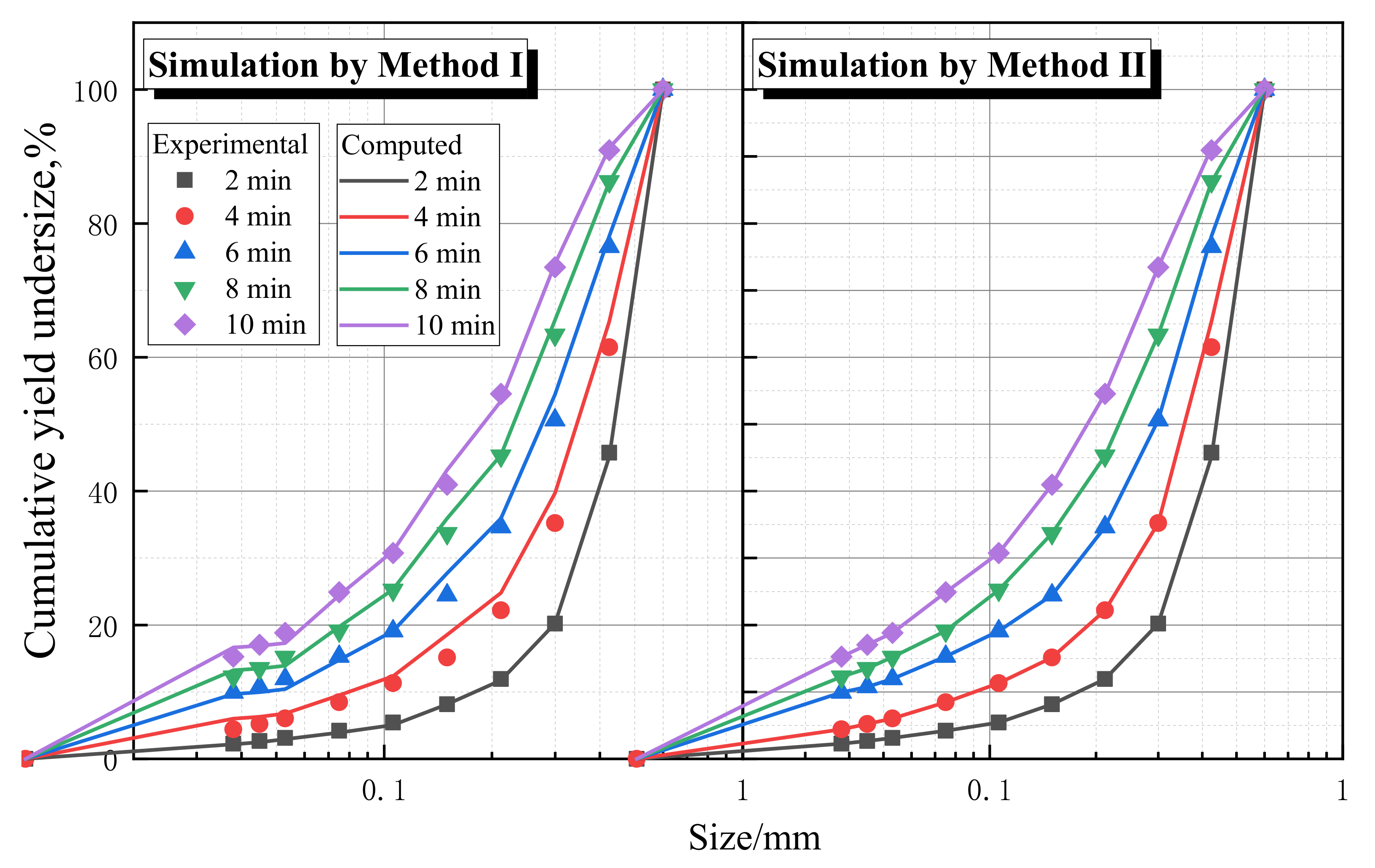
Simulation results and their fitting with the experimental data of −0.600 + 0.425 mm are shown in
Figure 8. Both methods obtained satisfactory fitting results, and the experimental data overlapped well with the calculated data from simulations, suggesting that in general, both methods could be used to describe the size characteristics of the grinding product. The curve obtained using the model of Method II was smoother than the fit of Method I because Method I involved iterative fitting, and the error was significantly magnified in the process of obtaining the two fits. In addition, when the model of Method I was used to predict the cumulative yield undersize for the fine particle size (less than 40 μm), there was a large relative error in the calculation of the cumulative distribution function, resulting in a relatively large error in the final fitting results.
Table 8 demonstrates a comparison between the results of simulation calculations and the actual experiment for each fraction using the two methods after grinding for 2 min. The maximum error between the simulation calculations and the experimental results did not exceed 1%, indicating that the value of fragmentation parameters of magnetite was correct. Therefore, it can be assumed that the mathematical models derived from the two methods can make theoretical predictions and determine the particle size characteristics of narrow-size magnetite grinding products.
The comparison results for when the grinding time was 4 min are summarized in
Table 9. The error of each size using Method Ⅱ was basically below 2% mass fraction, but the error of Method Ⅰ was around 3% mass fraction, especially for 0.300 mm with the error reaching 4.49% mass fraction. Overall, the fit of Method Ⅱ was significantly better than that of Method Ⅰ, and the prediction of the grinding product’s size characteristics was more accurate.
In general, compared with Method Ⅰ, this method demonstrates two merits. First, it demands less effort to calculate the value of the cumulative breakage distribution function (Bij), which greatly reduces the overall computational process and workload and thus generates higher fitting accuracy.
Second, the three parameters φ, γ, and β in Method Ⅰ had some errors in the fitting calculation, which caused a prediction bias [
15]. To reduce these errors, some scholars suggested that while calculating these parameters, the value of β could be first fixed according to the results generated by peer researchers, so that the other two parameters could be calculated. However, this effect is not obvious. Therefore, there are fewer derived parameters in Method Ⅱ for batch grinding, which means the number and degree of the error for each parameter are limited, and thus there would be less negative effect on the research of grinding characteristics. Additionally, it is worth mentioning that our recent studies have confirmed that Method Ⅱ is also more accurate for the case of wide-size grinding.
Third, given the previous two advantages, this method could be applied in studying the impact of parameters, such as rotational speed, diameter, etc., on the grinding status with a simpler process and higher accuracy.
However, as a new approach to grinding kinetics, Method Ⅱ has only proven its accuracy in batch grinding so far. Extensive work is still needed to verify its applicability in continuous grinding.


