Mapping Abandoned Uranium Mine Features Using Worldview-3 Imagery in Portions of Karnes, Atascosa and Live Oak Counties, Texas

Abstract

Worldview-3 (WV3) 16-band multispectral data were used to map exposed bedrock and mine waste piles associated with legacy open-pit mining of sandstone-hosted roll-front uranium deposits along the South Texas Coastal Plain. We used the “spectral hourglass” approach to extract spectral endmembers representative of these features from the image. This approach first requires calibrating the imagery to reflectance, then masking for vegetation, followed by spatial and spectral data reduction using a principal component analysis-based procedure that reduces noise and identifies homogeneous targets which are “pure” enough to be considered spectral endmembers. In this case, we used a single WV3 image which covered an ~11.5 km by ~19.5 km area of Karnes, Atascosa and Live Oak Counties, underlain by mined rocks from the Jackson Group and Catahoula Formation. Up to 58 spectral endmembers were identified using a further multi-dimensional class segregation method and were used as inputs for spectral angle mapper (SAM) classification. SAM classification resulted in the identification of at least 117 mine- and mine waste-related features, most of which were previously unknown. Class similarity was further evaluated, and the dominant minerals in each class were identified by comparison to spectral libraries and measured samples of actual Jackson Group uranium host rocks. Redundant classes were eliminated, and SAM was run a second time using a reduced set of 23 endmembers, which were found to map these same features as effectively as using the full 58 set of endmembers, but with significantly reduced noise and spectral outliers. Our classification results were validated by evaluating detailed scale mapping of three known mine sites (Esse-Spoonamore, Wright-McCrady and Garbysch-Thane) with published ground truth information about the vegetation cover, extent of erosion and exposure of waste pile materials and/or geologic information about host lithology and mineralization. Despite successful demonstration of the utility of WV3 data for inventorying mine features, additional landscape features such as bare agricultural fields and oil and gas drill pads were also identified. The elimination of such features will require combining the spectral classification maps presented in this study with high-quality topographic data. Also, the spectral endmembers identified during the course of this study could be useful for larger-scale mapping efforts using additional well-calibrated WV3 images beyond the coverage of our initial study area.

1. Introduction

Between 1955 and 2013, about 8% of total U.S. production of triuranium octoxide (U₃O₈) was extracted from an estimated 92 mines in Karnes, Live Oak and Atascosa Counties (the study area—Figure 1) in the Texas Coastal Plain [1]. These sandstone-hosted uranium roll front deposits were created when oxidized groundwater containing soluble uranium (e.g., U⁶⁺) interacted with organic- or sulfide-rich reducing zones in coastal marine sediments, where U-bearing minerals such as coffinite were precipitated ([1] and references therein). Much of this ore was recovered using open-pit mining (OPM) methods, commencing from the late 1950s/early 1960s until around the late 1990s, when in situ recovery (ISR) methods were developed (e.g., [1] and references therein). The legacy of uranium OPM is evident throughout the landscape, with numerous pit lakes, craters and waste piles scattered throughout Karnes and adjacent counties as a result. Some of these waste piles have been reclaimed using stabilizing vegetation cover, while others are more exposed due to constant erosion by water, wind and grazing animals. Notably, some of these waste piles may contain additional extractable critical and industrial mineral resources such as uranium, vanadium and zeolites (e.g., [2]). They can also pose radiological hazards if radioactive elements are concentrated at high enough levels (e.g., U, Th, Ra, Rn—[3,4,5]). In addition, these elements can lower the quality of surface water and groundwater due to acid mine drainage effects (e.g., [6] and references therein). Therefore, there exists a need for inventorying the locations of these exposed waste piles, as well as their bedrock source areas.

Prior to the advent of advanced multispectral and even hyperspectral sensors, some of the earliest applications of multispectral remote sensing imagery (e.g., Landsat Multispectral Scanner (MSS)) for uranium mineral exploration relied heavily on the detection of ferric iron minerals associated with roll-front and sandstone-hosted deposits (e.g., [9,10,11]). However, those studies were not specifically targeting active mines and/or waste piles. After reviewing the criteria for using spaceborne multispectral and hyperspectral imagery for identifying uranium mines and mills, Stork et al. [12] concluded that uranyl-bearing minerals tend to occur in concentrations too low to be detected. They also noted that spectrally more abundant gangue minerals would have to be used instead. Some of the earliest hyperspectral studies demonstrated the utility of aircraft-flown airborne visible/infrared imaging spectrometer (AVIRIS) data for characterizing the type, distribution and abundance of alteration (and some gangue) minerals in mine waste, as well as downstream ferruginous sediments and resulting acid-mine drainage and runoff (e.g., [13,14,15,16]). However, these and other multi- and hyperspectral studies reviewed by Werner et al. [17] focused mainly on the land-use, water quality and human health impacts of individual mine sites, and did not necessarily focus on broader regional mapping such as across entire watersheds (e.g., [18]) or even inventorying multiple waste piles and/or mine features.

Although there have been other attempts at inventorying past and currently operational open-pit mines and uranium mineral occurrences along the South Texas Coastal Plain and elsewhere (e.g., [1,19]), those efforts have relied on information extracted from historic topographic maps and/or provided by lease holders and property owners to state regulatory agencies such as the Railroad Commission of Texas. Unfortunately, many of the mines are often inaccurately located and their waste piles are often transported miles away from their original excavation sites [1]. Also, a number of these waste rock and tailings piles may not have been recorded at all. In this study, we demonstrate the use of 16-band multispectral imagery (i.e., Digital Globe Worldview-3, herein WV3) for extracting spectral signatures from known open-pit mine bedrock exposures and waste piles and using them to identify spectrally similar target features elsewhere throughout the image. In the process, we also show how these spectral signatures can be used to distinguish bedrock and mine waste materials from other regolith and landscape surface features which may share subtly similar spectral characteristics, such as bare and fallow agricultural fields and oil and gas drill pads. The resulting spectral classification maps can be combined with other data and/or used as a basis for more accurate inventories of the locations of uranium mine excavations and their resulting waste piles.

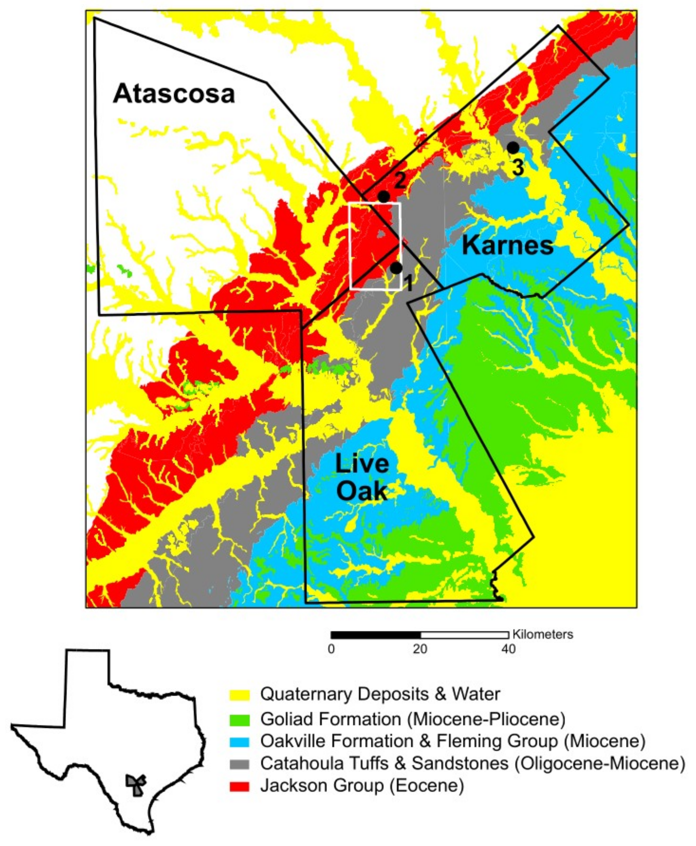
2. Study Area: Location, Geology, Soils, Vegetation, Land-Use and Land-Cover

Our study area encompasses portions of Karnes, Live Oak and Atascosa Counties, and is covered by an ~11.5 km wide by ~19.5 km long WV3 satellite image (white rectangle—Figure 1 and Figure 2a) acquired on 12 October 2017. Much of the bedrock shown to be exposed and mined within the image coverage area consists of sedimentary rocks from the Jackson Group, with some overlying cover of rocks and sediment from the Catahoula Formation (Figure 1). The Eocene Jackson Group is geologically the oldest Gulf Coastal Plain sedimentary unit from which uranium has been mined [2]. It consists predominantly of quartzo-feldspathic sandstone, mudstone, claystone and lignite members, whose origins are coastal strandplain/barrier bar sand bodies as well as lagoonal mud and swamp deposits, minor landward fluvial channel sand bodies and gulfward shelf-related mud deposits [20,21]. Several members of the Jackson Group are described as tuffaceous in origin, with some members described as fossiliferous and bentonitic ([7,21] and references therein). The Oligocene to Miocene Catahoula Formation consists mainly of tuffaceous mudstone, claystone, sandstone and conglomerate members, and is interlaminated with massive and less altered volcanic tuff deposits of rhyolitic, trachytic and trachyandesitic composition ([7,22] and references therein). The Catahoula Formation is believed to be the main source of the uranium mined in the area, in that it has been heavily leached of uranium by oxidizing and alkaline groundwaters, which deposited the uranium in reducing zones surrounded by impermeable barriers. Some of these reduced or “roll front” zones are contained within the Catahoula itself, as well as underlying (Jackson Group) and overlying (Oakville Formation) geologic units ([1,2,22,23] and references therein). Smectitic soils dominate the area, according to previous soil surveys ([24]—Figure 2d), which is not surprising, since the parent bedrock material is dominated both spectrally and mineralogically by montmorillonite (e.g., [2]).

Prior to this study, 23 known mines and occurrences (larger black circles—Figure 2c) were compiled by Hall et al. [1], all of which were mined within and/or are associated with Jackson Group rocks at depth. This includes the “Esse-Spoonamore” mine (labeled as 1—Figure 1), which is covered within our imagery, but was mined beneath a surface cover of Catahoula. An additional 24 possible mine locations (smaller black circles—Figure 2c) were digitized directly from 7.5 min historic topographic maps compiled by Horton and San Juan [19]. Seven of these points located within Live Oak County were attributed as “gravel pits”, while the remaining seventeen points located within Karnes and Atascosa Counties were attributed as “quarries”. Interestingly, some of the points digitized from the topographic maps either overlapped with or were in close proximity to the uranium mines and occurrences compiled by Hall et al. [1]. Several of these abandoned open-pit mines have left evidence on the landscape in the form of numerous craters, some of which are permanently or seasonally filled with pit lakes (Figure 2a,b); nearby piles of waste rock and mine tailings can be recognized as well. In addition to historical uranium mining, the production of other energy resources such as lignite coal bed mining (e.g., [29]) and oil and gas drilling have left evidence on the landscape. For example, there are numerous bright and rectangular-shaped drill pads visible within our satellite imagery (Figure 2a), especially near major and secondary roads. Notably, much of the oil and gas production in the area is associated with the much deeper Upper Cretaceous Eagle Ford Shale Play (e.g., [30,31] and references therein).

One striking feature of our WV3 image (Figure 2a) is the abundant vegetation cover, which appears as various shades of green in the composite of visible bands displayed. Notably, not all the abandoned mine features in the area are well exposed, and several have since been fully or partially reclaimed by the growth of natural and/or anthropogenically planted vegetation. Some of this vegetation includes crop- and pastureland (Figure 2b). The analysis of temporal changes in vegetation cover and/or distinguishing reclaimed abandoned mine features from non-reclaimed or even active features is beyond the scope of this work (see, e.g., [32,33]). However, three different GIS datasets compiled at different times and which use different methods show good agreement in the distribution of natural and artificially planted vegetation types found throughout our study area. For example, the 2016 National Landcover Database (NLCD—[25]) shows that approximately 55% of our study area is covered in shrub/scrub vegetation types, 32% is covered by hay and pastureland and around 7% is covered by cultivated crops (Figure 2b and Supplementary Materials Table S1a). The 2017 Texas Cropland Data [34] also shows around 55% of the area covered in shrubland, but breaks the artificially planted and fallow vegetation types further into 26% grassland pasture; 6% non-alfalfa hay; and various crop types, including around 2% each for oats and corn, 1.5% cotton, and nearly 1% fallow or idle cropland (Supplementary Materials Table S1b). The Texas Parks and Wildlife “Vegetation Types of Texas” map [35] and updated vector GIS database [36] provide the best information on naturally occurring native and invasive shrubland communities in our study area. For example, the three largest communities based on aerial coverage percentages are “South Texas Disturbance Grassland” (~46%—Supplementary Materials Table S1c,d), “South Texas Clayey Mesquite Mixed Shrubland” (~13%—Supplementary Materials Table S1c,d) and “South Texas Shallow Shrubland” (~7%—Supplementary Materials Table S1c,d). In all three shrubland types, honey mesquite (Prosopis glandulosa) is the typical and most dominant overstory vegetation type, while common understory species can include Cynodon dactylon (bermudagrass), Acacia farnesiana (huisache), Celtis ehrenbergiana (granjeno), Acacia rigidula (blackbrush), Pennisetum ciliare (buffelgrass) and Ziziphus obtusifolia (lotebush), to name a few (e.g., [36]). Notably, planted row crops are estimated at around 6% aerial coverage (Supplementary Materials Table S1c,d), which agrees somewhat with the NLCD dataset (Figure 2b). Inherent within our methodology is the masking of all vegetation and artificially built-up surfaces (e.g., red colored pixels—Figure 2b) in order to facilitate the extraction of spectral signatures (i.e., endmembers) that can be used to map mine waste material and source bedrock. These procedures are described in further detail in the following section.

3. Image Calibration, Pre-Processing, Spectral Analysis and Classification Methods

Considerable portions of the methods used for atmospheric correction and calibration of WV3 radiance data to reflectance closely follow those presented by Mars [37]. The pre-processing steps include spectral and spatial data reduction and extraction of spectral endmembers through multi-dimensional class segregation methods, which follows the “spectral hourglass” approach described in greater detail by Boardman and Kruse [38] and the references therein. In summary, WV3 data were distributed as two VNIR (spectral bands between 400 and 1000 nm) and one SWIR (spectral bands between 1000 and 2500 nm) scenes with overlapping spatial coverage. The two VNIR scenes covered both the northern and southern halves of the geographic extent (white outline) shown in Figure 1, respectively, while the SWIR scene covered the entire extent of the study area. The ~3.9 m resolution SWIR pixels were resampled to the ~1.3-m resolution VNIR pixels so that both datasets could be spectrally joined to form a continuous 16-band spectral dataset (e.g., [37,39]). WV3 had 8 VNIR spectral bands at approximately 429, 483, 548, 605, 661, 723, 825 and 914 nm; and 8 SWIR spectral bands at approximately 1210, 1572, 1662, 1730, 2164, 2203, 2260 and 2330 nm. The VNIR subset had bands in common with previous sensors such as the Advanced Land Imager (ALI) and Sentinel, while the SWIR subset had bands in common with ASTER (e.g., [37,39]), but both at much higher spatial resolutions. Despite the system not being hyperspectral, Mars [37] showed that WV3 can be used to produce comparable mineral maps, provided that overlapping spectral absorption features are considered for mineral groups.

The FLAASH atmospheric correction program [40], available as a module within the Environment for Visualizing Images (ENVI—[41]) software, was used to convert the VNIR and SWIR radiance values of WV3 to scaled reflectance. Atmospheric correction was first performed using an initial scene-dependent and software-derived estimate of atmospheric water vapor. This was later revised based on more reliable total precipitable water vapor values (scene average = 5.5 cm) derived from the MODIS satellite sensor, which were acquired within an hour of the WV3 image (e.g., [37]). The resulting 16-band reflectance dataset was then used for further pre-processing, including vegetation masking and the removal of noisy and/or outlier pixels and artificial surfaces not related to exposed rocks or natural regolith materials. With 16 spectral bands spanning the VNIR and SWIR wavelengths, several green and dry vegetation indices can be derived, as was summarized and reviewed by Hively et al. [42]. The standard normalized difference vegetation index (NDVI) and the shortwave infrared normalized difference residue index (SINDRI) were used to map green chlorophyll-bearing and senesced lignin- and cellulose-bearing materials, respectively (results shown separately in Supplementary Materials Figure S1). The NLCD (Figure 2b) was used to help to facilitate the masking of artificially built-up and impervious surfaces such as roads, building rooftops and parking lots, with the help of Google Earth imagery acquired around the same time as the WV3 image.

After vegetation masking, a minimum noise fraction (MNF) procedure was applied to the remaining WV3 pixels. The MNF transformation is a variation of the standard principal components analysis (PCA) procedure, which relegates spatially incoherent noise to higher-order image channels that have been transformed to an orthogonal feature space, thus allowing for noise and data redundancy to be excluded from subsequent analyses [43]. Boardman and Kruse [38] highlight this as an essential step for spectral compression, noise suppression and dimensionality reduction (e.g., [39]). They also describe further spatial data reduction by applying a pixel purity index (PPI) to the remaining non-masked pixels. PPI uses convex geometric methods [44] to determine which pixels have the most extreme spectral features and are, therefore, considered to be the “purest” and thus most useful as spectral “endmembers” ([38] and references therein). Figure 2c shows the location and distribution of 943 WV3 pixels identified as spectral endmembers using the PPI method. Notably, these pixels are considered “pure” in a macroscopic sense if they are homogeneous targets. Therefore, their resulting spectra can be combined in a linear mixing fashion (i.e., through spectral averaging or weighted proportions) to explain every remaining spectral signature in the data [38]. Alternatively, intimate mixtures behave non-linearly at sub-pixel scales (e.g., [38,45] and references therein). Even prior to subsequent processing and spectral analysis, these pixels were evaluated as legitimate targets based on their locations on exposed fresh bedrock, possible abandoned mine materials and/or weathered bedrock and regolith materials using Google Earth imagery.

The next pre-processing step involved separating and clustering the 943 PPI-derived pixels into spectral classes using n-dimensional visualization methods, where “n” equaled the number of spectral bands containing spatially and spectrally coherent information, as opposed to various types of noise (e.g., [38,41,44]). Notably, the n-dimensional orthogonal feature space defined during the MNF processing step also defined a “mixing space” where pixels located further from the center were considered less mixed ([38] and references therein). In this case, the 943 pixels shown in Figure 2c actually represent 6% of a larger subset of PPI-mapped pixels, most of which were plotted much closer towards the center of the 16-band orthogonal feature space. Likewise, the spaces further from the center where these pixels clustered together can be considered spectral classes, each displaying different spectral shapes from one another ([38] and references therein). Using this n-dimensional visualization method, all 943 PPI-mapped pixels were segregated into 58 unique spectral classes, which were then evaluated further. 16-band WV3 spectra representing each of these 58 spectral classes are shown and provided in Supplementary Materials Table S2.

Boardman and Kruse [38] note that the automated identification of spectral endmembers “is still problematic”, and most methods require comparing absorption features displayed within endmember spectra to those of material standards available within spectral libraries (e.g., [46]). These methods can be either manual, such as visual comparison and interpretation of spectral absorption features, or automated by use of spectral shape-fitting algorithms, such as the spectral angle mapper (SAM) or the USGS Tetracorder and Material Identification and Characterization Algorithm (MICA) codes ([47,48,49,50] and references therein). For this study, we compare our WV3 image endmembers to around 70 laboratory spectral measurements of rocks and sediments, mostly from the Jackson Group, collected from seven former uranium open-pit mine locations. These samples were measured using a portable FieldSpec4 Analytical Spectral Device (ASD—Model #18336) with an artificial light probe attachment (model #A122320), which measures continuous spectral reflectance in the range of 350–2500 nm at ~1 nm spacing. Prior to being convolved to the broader VNIR and SWIR bandpasses of WV3, the full-spectral-resolution ASD-derived spectra were analyzed using MICA in order to determine the spectrally most dominant minerals in the 1- and 2-micron wavelength regions. The mineral identification command file governing the execution of MICA included ferric iron minerals in the 1-micron VNIR range, as well as clay, sulfate and carbonate minerals in the 2-micron SWIR range (e.g., [51]). Sample spectra from three of these mine sites that best match the spectral shapes of our image endmembers (black filled circles—Figure 1) are compiled and summarized here in the results section for both clarity and brevity. The SAM methodology used to compare the endmember spectra with the convolved laboratory sample spectra described above is further discussed below. Also, the full-resolution version of each mine site sample spectrum is provided in a separate data release publication [8].

The SAM method determines the similarity between two spectra in n-dimensional feature space (i.e., n = 16 for WV3) by treating them as vectors and computing the angle between them. This angle is based on the arc-cosine of the dot product of the two spectral vectors [47]. The smaller the computed angle, the closer the match in spectral shape between the two spectra. SAM has an added benefit in that it is insensitive to brightness or albedo differences between the two spectra being compared. This is because the computed angle between the two spectra is independent of the lengths of the vectors used to calculate the angle between them in the first place. Typically, SAM is run on either hyperspectral or multispectral data by comparing image pixel spectra to reference spectra from a spectral library (e.g., [46]). Crosta et al. [48] provide a more detailed summary and comparison of the SAM and Tetracorder methods, on the latter of which MICA is loosely based, as well as discussing their resulting classification accuracies using actual hyperspectral imaging spectrometer data. For this study, we used the SAM algorithm in different ways for three different purposes. For example, spectral angle measurements of similarity were computed for each of 58 spectral class endmembers as pairs against one another and compiled in a matrix format, along with their standard deviations from the average computed spectral angle value (Supplementary Materials Table S3). This was carried out in order to help to evaluate which of these spectral signatures varied only subtly, if at all. Secondly, SAM was also used to compare each of the 58 spectral endmember classes to a library of 70 laboratory-measured spectra of MICA-characterized Jackson Group rock cores, as described above. Those results are discussed further in the section below. Finally, both the original set of 58 spectral endmembers (Figure 2c) and another set which was reduced to 23 endmembers were used as inputs for SAM classification of the entire WV3 scene (Figure 2a). Both sets of results were compared to one another, and the overall accuracy of the mapping results were further evaluated in the context of landscape features that we expect will impart some confusion to the accuracy of our mapping results (e.g., bare agricultural fields and oil and gas drilling pads). This is in spite of the fact that most of our spectral endmembers closely match the spectral characteristics of host Jackson Group sedimentary rocks. In our evaluation of accuracy, we also considered the mapped spatial distribution of individual spectral classes across previously located and/or field-investigated mine and waste pile features (e.g., [1,52,53]).

4. Results

4.1. Compositional Identification of Spectral Endmembers

All 58 spectral endmembers were compared to higher-resolution (>1000 bands) spectra convolved to the 16-band spectral resolution of WV3. These include all the Jackson Group rocks described above and measured at the Texas Bureau of Economic Geology core facility in Austin, Texas [8], as well as pure mineral standards compiled in the USGS spectral library [46]. Using the SAM algorithm and the default threshold matching vector angle of <0.10 radians, 62% of our spectral endmembers were matched to the spectra of 15 Jackson Group rock samples (

Table 1. Spectral endmembers matched various rocks and sections of Jackson Group core material measured in the laboratory [8]. Spectral endmembers 5 and 14, shown in bold text, were extracted from the McCrady waste pile, while endmembers 22 and 24 (also shown in bold text) were extracted at or near the Garbysch-Thane mine, as discussed in portions of the text.

Endmember Class #	Spectral Match Angle (Radians)	Spectral Match (Geologic Sample)	1-Micron MICA Match	2-Micron MICA Match
33	0.058535	bargmann-1	goethite.thincoat.singlefeat	montmorillonite_Na_highfit
25	0.066616
19	0.068115
48	0.090795
43	0.045664	bargmann-2	goethite.thincoat.singlefeat	kaolin.5+smectite.5
34	0.070265
45	0.089269
35	0.069281	spoonamore-4	lignite (nanohematite.singlefeat false positive)	montmorillonite_Na
36	0.074693
41	0.079308
49	0.080826
24	0.077495	spoonamore-5	goethite.thincoat.singlefeat	montmorillonite_Na_highfit
5	0.085778
39	0.092893
29	0.088401	spoonamore-6	Unclassified	montmorillonite_Na
13	0.058144	spoonamore-7	goethite.thincoat.singlefeat	montmorillonite_Ca
55	0.090287
37	0.065497	spoonamore-9	lignite (hematite.finegr.fe2602 false positive)	Unclassified
30	0.085383
52	0.096045
54	0.073947	spoonamore-10	lignite (nanohematite.singlefeat false positive)	Unclassified
40	0.07803
58	0.079606
11	0.08331
50	0.085465
44	0.053086	spoonamore-12	Unclassified	montmorillonite_Na
23	0.076721
1	0.084202	spoonamore-13	lignite (nanohematite.singlefeat false positive)	montmorillonite_Na
28	0.044385	spoonamore-14	Unclassified	montmorillonite_Na
57	0.052872	spoonamore-27	Unclassified	chalcedony
22	0.069876
14	0.081956	spoonamore-38	Fe3+_type_1b (Acid_Mine_Dr Assemb1)	montmorillonite_Na_highfit
12	0.033884	winerich-5	goethite.thincoat.singlefeat	montmorillonite_Na
17	0.035235
42	0.06012
27	0.036447	winerich-8	Unclassified	calcite.8+montmorillonite_Ca.2

). For convenience, Table 1 also provides the corresponding 1- and 2-micron MICA-generated mineral identification results [8]. The latter MICA analyses used the higher-spectral-resolution versions of each spectrum. For brevity, five of the best matches (i.e., <0.077 radian- computed vector angles and visual interpretation) are shown in Figure 3, with Figure 3a showing the image-derived spectral endmembers on the left and Figure 3b showing the resampled Jackson Group rock spectra described in Table 1 on the right. In all cases, the 2-micron (i.e., >2000 nm, or SWIR range), mostly montmorillonite clay absorption features (2203 nm) were well-resolved by WV3 in both sets of spectra. The Spoonamore-27 spectrum (blue plot—Figure 3b), on the other hand, was dominated by a hydrous silica mineral feature (2260 nm) matched to chalcedony during the full-resolution MICA analysis. This feature was also resolved less strongly within the image endmember represented by class 57 (blue plot—Figure 3a). The 1-micron (i.e., <1000 nm, or VNIR range) iron-bearing minerals were typically not as well resolved due to a combination of fewer spaced-out WV3 bands in that spectral region and the broader shapes of iron-bearing minerals responsible for those features, such as hematite, goethite and jarosite (e.g., [37,39]). In this case, Jackson Group rocks were dominated mainly by goethite and lignite features, as shown in Table 1. Except in cases where there is interference from chlorophyll-bearing vegetation, WV3 image spectra strongly affected by ferric iron minerals (and/or lignite) generally shows a strong slope from WV3 bands 6 to 1 (723 to 429 nm). Notably, the image endmembers shown in Figure 3a differ from the rock spectra shown in Figure 3b in that they display weak residual chlorophyll features due to subtle mixing with unmasked residual vegetation material at the surface. This demonstrates that even the most homogeneous remote sensing pixels are rarely pure, considering how prevalent aerial mixtures with vegetation are on earth.

The remaining 38% of our spectral endmembers were not matched to any of the rocks from the Jackson Group or any other geologic units exposed in the area (Figure 1), despite consistently using the same SAM default vector angle threshold of <0.10 radian. However, each spectrum was visually compared to absorption features associated with minerals within a convolved version of the USGS spectral library [46], as well as spectra measured and/or digitized from other sources, such as lignite coal (e.g., [54]) and the uranium mineral coffinite (e.g., [55]). Other minerals detected in the samples and cores of Jackson Group rocks using higher-resolution spectral measurements [8] include gypsum, jarosite and calcite mixtures with montmorillonite. A detailed summary of the characteristics of these endmembers and a supporting discussion of the suitability of each for further classification of mine waste features throughout the rest of the image is provided in Supplementary Materials Table S4. Examples of endmembers displaying three of the most commonly identified and sometimes ambiguous spectral features summarized in Supplementary Materials Table S4 are shown in Figure 4. For example, endmember 3 (green plot—Figure 4a) shares some spectral shape characteristics with a convolved gypsum spectrum from the USGS spectral library (green plot—Figure 4b), except for the drop in reflectance of the last band displayed by endmember 3. This includes a prominent reflectance peak in WV3 SWIR band 3 (1662 nm) and a broad flat absorption feature at SWIR band 6 (2203 nm), with a steep slope between both wavelength bands. However, image endmember 3 displays an additional drop between SWIR bands 7 and 8 that is likely due to mixing with carbonate minerals such as calcite, as well as a residual chlorophyll feature in VNIR band 5 (661 nm) from mixing with unmasked vegetation. Image endmember 56 (red plot—Figure 4a) matches well with the lignite coal spectrum presented in Kruger et al. [54] (red plot—Figure 4b). In fact, a spectral angle of similarity of ~0.08 radian (less than the 0.10-radian SAM default threshold) was calculated between the two spectra. In coal and other hydrocarbon materials, this broad concave-shaped feature continues into the ultraviolet and is due to electronic transitions in complex organic molecules (e.g., [56]). However, the image spectrum (red plot—Figure 4a) displays an additional sharp absorption feature at 2203 nm due the presence of montmorillonite and a weak chlorophyll feature, both of which are absent in the reference lignite spectrum (red plot—Figure 4b).

An example of a more ambiguous spectral feature is illustrated by the absorption feature displayed in SWIR band 1 (1210 nm) of image endmember spectrum 20 (black plot—Figure 4a). Several minerals display absorption features broad and deep enough to overlap with WV3 SWIR band 1 (1210 nm), including zeolites (~1157 nm) and the uranium mineral coffinite (~1135 nm) (e.g., [8]). In the case of coffinite and other uranium minerals, Dahlkamp [2] notes that abundances in South Texas deposits typically do not exceed 1000 ppm or <0.1 wt%, although the highest-grade ores can contain up to 0.3 wt% or 3000 ppm (e.g., [1,57]). Herbert et al. [55] measured the VNIR-SWIR reflectance of coffinite, including various mixtures with silica sand, and showed how various absorption features decreased in depth between 0 and 1 wt%. The strongest coffinite absorption feature at ~1135 nm was still detectable above instrument background noise down to >0.1 wt%. Figure 4b shows the pure coffinite spectrum measured by Herbert et al. [55], convolved to WV3. Notably, the broad and deep feature at 1135 nm is diminished to a weaker absorption feature at WV3 SWIR band 1 at around 1210 nm, as compared to the WV3 image endmember 20 shown in Figure 4a. Also, the continuum slope of the pure coffinite feature (Figure 4b) goes from being brighter at longer wavelengths to less bright at shorter wavelengths, which is the reverse of the continuum slope displayed by the WV3 image spectrum (black plot—Figure 4a). Unfortunately, Herbert et al. [55] did not provide digital versions of their spectra. Therefore, the shape of the spectral absorption features depicted in Figure 4b may not be accurate due to the lack of reference scales on the plot figures rendered by these authors.

Zeolite minerals such as heulandite and/or clinoptilolite also occur within Jackson Group rocks [2,21,22,23,29]. Figure 5a shows three example spectra from the Spoonamore mine site, which all display weak zeolite-related absorption features at 1157 nm. However, absorption feature depth analysis [58] of these and two other Spoonamore rock samples displayed weaker absorption features with lower relative band-depth (RBD) values at 1157 nm (

Table 2. Spectral endmembers with high relative band depth (rbd) values indicative of absorption features in WV3 SWIR band 1 (1210 nm) that may be due to zeolite minerals computed in the last column using full-resolution (i.e., hyperspectral) spectra of the Jackson Group rock sample shown in column 3. Spectral endmembers 5 and 20, shown in red, were extracted from the McCrady waste pile, as discussed in portions of the text. See also Table 1 for the MICA mineral matches to the geologic samples shown in column 3. Supplementary Materials Table S4 describes the endmembers listed as “unmatched”. “#” refers the n-dimensionally clustered class numbers discussed throughout the text.

Endmember Class #	WV3 rbd-1210 nm (Zeolite/Uranium Minerals Index)	Spectral Match (Geologic Sample)	Hyperspectral rbd-1157 nm (Heulandite/Clinoptilolite)
21	2.478887	unmatched	N/A
32	2.344082	unmatched	N/A
20	2.186793	unmatched	N/A
15	2.150885	unmatched	N/A
2	2.147810	unmatched	N/A
29	2.103521	spoonamore-6	2.017605
8	2.053413	unmatched	N/A
55	2.047738	spoonamore-7	2.004085
5	2.044193	spoonamore-5	2.028697
23	2.036904	spoonamore-12	2.035804
50	2.027945	spoonamore-10	2.012043
56	2.012584	unmatched	N/A
47	2.010877	unmatched	N/A
31	2.006367	unmatched	N/A

) than the RBD values computed using SWIR band 1 for WV3 spectral endmembers matched to Spoonamore samples and others (Table 2). Notably, none of the zeolite features displayed in the spectra of higher spectral resolution (Figure 5a) were preserved when these spectra were resampled to the lower spectral resolution of WV3.

Another possible explanation for the broad and deep features at 1210 nm, as exemplified by image spectral class 20 (black plot—Figure 4a), are intimate mixtures of the sulfate minerals gypsum and jarosite, both of which have been reported in Jackson Group rocks, including iron disulfide minerals, of which they are alteration products (e.g., [2]). Evidence of this is provided by the higher-spectral-resolution spectrum of gypsum shown in Figure 5b, which displays a fairly strong absorption feature at ~1204 nm. However, when convolved to the spectral resolution of WV (top red plot—Figure 5b), this feature becomes overwhelmed by the steep continuum slope towards the triplet-shaped absorption feature at 1444 nm. On the other hand, image spectral class 20 (black plot—Figure 4a) shares similar shape attributes with the jarosite spectrum convolved to WV3, including a steep continuum slope from WV3 VNIR bands 6 to 1 (723 to 429 nm) due to ferric iron. However, the full-resolution jarosite spectrum (bottom black plot—Figure 5b) displays an absorption minimum at 914 nm (VNIR band 8) when convolved to WV3 (upper black plot—Figure 5b), which is shifted from the absorption minimum at 1572 nm (SWIR band 2) displayed by the WV3-convolved version of gypsum (top red plot—Figure 5b). Unfortunately, current spectral libraries do not contain reference spectra for various mixtures of gypsum and jarosite. Although the exact nature of the mixing (e.g., aerial versus intimate) between gypsum and jarosite in our study area is unknown, numerous studies of lignite and uraniferous lignite-bearing mine waste support our intimate mixing interpretation, with several of these studies documenting various proportions and abundances of the two minerals (e.g., [54,59,60,61]).

4.2. SAM Initial Classification Results, Class Reduction and Accuracy Assessment

All 58 initial endmember spectra were used as inputs for SAM classification of the entire WV3 scene using the default threshold of 0.10 radian. Figure 6b shows those results, although the assigned colors are too numerous to label at the scale shown. For reference, Figure 6a shows a larger version of the visible band color composite of the full WV3 scene shown in Figure 2a, likewise showing the locations of 23 previously known mine sites (red filled circles) compiled by Hall et al. [1]. In total, we located at least 117 suspected mine-, quarry- and waste-related features in the landscape (yellow open circles—Figure 6a). This is largely based on our knowledge of previously known mine, waste pile and pit crater locations, as well as photo-geologic interpretations of the spatial patterns and distribution of mapped classes derived from each of the spectral endmembers. At least 22 of these features either are close to (i.e., <200 m) or cover some of the known mines, prospects, occurrences and quarries mapped by Hall et al. [1] and/or Horton and San Juan [19] within their boundaries.

In addition to in situ bedrock and translocated mine waste rock-related features, SAM classification (Figure 6b) also highlights and maps large areas of exposed bare ground associated with agricultural fields (crop and pastureland—Figure 2b), as well as numerous oil and gas drill pad features. This is not surprising because many of the soil series exposed throughout Karnes, Atascosa and Live Oak Counties are young, having formed in a semi-arid climate, and tend to have poorly developed organic-rich O horizons (i.e., topsoil). Therefore, their mineralogy tends to reflect that of the parent lithologies on which they are developed, but modified by the addition of carbonate minerals and/or gypsum (e.g., [26,27,28]). In particular, Molina [27] mapped several uranium mine pits and dumps throughout Karnes County and noted that “areas of piled soil material are 50 to 100 feet higher than the natural surface elevation and consist of original topsoil that has been mixed with the parent material”. In the case of oil and gas drill pad features, the original topographic surfaces are often leveled and compacted by clearing the original vegetation and underlying topsoil, with the latter often being stored elsewhere for later landscape restoration (e.g., [62,63,64] and references therein).

Table 3. Class histogram statistics, sorted by % of total mapped pixels (see Supplementary Materials Table S5a–e for full expanded statistical dataset), for various broad and generalized land-use and land-cover categories. Bare and partially fallow fields; oil and gas drill pads; and exposed bedrock (usually along pit craters), waste piles and quarries were all identified by photo-geologic interpretation of true-color WV3 imagery and sampled randomly using region of interest (ROI) polygons, while avoiding edges and mixtures. Class numbers in bold are based on endmembers extracted from the Wright-McCrady mine area, as discussed in Section 4.3 of the text. Other endmembers (i.e., numbers 22, 24 and 38) extracted from the Esse-Spoonamore and Garbysch-Thane areas map fewer pixels, as explained in the text, but their full scene statistics are included in Supplementary Materials Table S5a–e. “#” refers the n-dimensionally clustered class numbers discussed throughout the text.

58 EMs Full WV3 Scene		58 EMs Bare/Partially Fallow Fields		58 EMs Oil/Gas Drill Pads		58 EMs Bedrock/Mine /Quarry Features		23 Reduced EMs Full WV3 Scene
Class #	% Mapped	Class #	% Mapped	Class #	% Mapped	Class #	% Mapped	Class #	% Mapped
35	17.57	54	29.95	13	42.08	35	16.79	35	25.04
54	13.25	11	14.22	57	20.62	26	14.59	54	23.30
26	11.36	35	13.00	44	12.28	53	12.84	37	10.43
53	7.54	37	8.43	28	7.98	57	8.15	14	6.85
11	5.77	43	6.13	27	6.54	14	6.74	13	5.82
37	5.60	26	5.59	19	2.34	37	4.52	25	5.30
13	4.96	58	5.57	17	2.10	13	4.03	57	4.66
58	4.05	40	4.67	16	0.99	36	2.86	43	3.33
25	3.81	50	2.60	37	0.60	5	2.67	44	2.99
57	3.57	56	2.48	36	0.56	19	2.61	56	2.66
43	2.72	25	2.40	30	0.39	58	2.47	1	2.50
40	2.17	45	1.49	29	0.33	25	1.97	28	1.43
44	1.96	48	0.72	43	0.27	54	1.79	5	1.24
28	1.21	12	0.59	52	0.26	48	1.37	12	1.21
56	1.16	10	0.37	31	0.24	28	1.28	51	0.98
14	1.14	53	0.33	54	0.21	33	1.15	27	0.87
50	1.05	51	0.25	12	0.20	44	1.14	29	0.65
48	0.94	19	0.22	26	0.20	42	1.08	20	0.61
27	0.74	42	0.20	42	0.19	20	1.00	32	0.10
33	0.69	1	0.15	14	0.18	49	0.83	2	0.02
19	0.66	49	0.12	53	0.15	17	0.83	15	0.01
45	0.63	36	0.12	5	0.15	29	0.80	21	0.01
5	0.60	9	0.09	25	0.15	39	0.75	3	0.00

provides a partial summary of histogram statistics for pixels classified by SAM as matches for many of the top 23 of 58 endmember classes. The full statistical dataset is provided in Supplementary Materials Table S5a–e. In addition, pixels were randomly sampled from features positively identified as either: (1) bare or partially fallow fields with exposed underlying weathered regolith materials (~31% of classified pixels); (2) rectangular-shaped oil and gas drill pad features (~5% of classified pixels); and (3) bedrock-, quarry- or mine-related features (~2% of classified pixels). Histogram class statistics for these features are also provided in Table 3, with the full expanded versions provided in Supplementary Materials Table S5a–e. These supplemental tables also provide average spectra for each of the three land-use categories for pixels mapped as any of the full 58 endmember classes.

The top three classes mapped throughout the full WV3 scene (column 2—Table 3) were based on endmembers 35, 54 and 26, each mapping more than 10% of the total classified pixels. Both classes 35 and 54 matched well to two convolved spectra measured from rock materials sampled from the Spoonamore mine (Table 1). In both cases, their spectral signatures were dominated by lignite, but differed in that the class 35 input spectrum exhibited an additional absorption feature related to montmorillonite, while class 54 did not (Table 1). Although both input spectra had similar shapes due the presence of lignite or spectrally similar materials, the spectral angle calculated between the two reference spectra was 0.156 (Supplementary Materials Table S3), which is larger than the 0.100 SAM threshold used for classification purposes due to the detection of stronger montmorillonite absorption features in class 35 pixels. Class 54 was notably the largest percentage of pixels mapped which represented bare or partially fallow crop- and pastureland (columns 3 and 4—Table 3). Class 35 ranked highest as a percentage of all pixels classified for the whole scene (columns 1 and 2—Table 3), as well as pixels covering only rock, mine or quarry features (columns 7 and 8—Table 3), using all 58 endmembers as SAM inputs. However, class 35 also mapped 13% (3rd highest) of the classified pixels covering bare or partially fallow crop and pastureland (columns 3 and 4—Table 3). Class 26 did not match to any of the WV3 convolved spectra of Jackson Group rocks sampled from various mine sites (Table 1), but did display both a slight chlorophyll feature from unmasked vegetation and a strong montmorillonite feature (Supplementary Materials Table S4). It was included in the initial classification, which used all 58 endmembers as inputs, but was later excluded in the second classification attempt (column 9—Table 3), as explained further below. Notably, class 26 had the second-most classified pixels, covering bedrock, mine and quarry features during the initial classification run using all 58 endmembers (columns 7 and 8—Table 3).

Class 53 yielded the third highest percentage of classified pixels, covering mine, quarry and bedrock features (columns 7 and 8—Table 3). Like class 26, it did not match to any of the Jackson Group rocks from the mines listed in Table 1 or elsewhere. Also, its input endmember spectrum appeared to be dominated by weak, dry vegetation features, as described in Supplementary Materials Table S4. Class 11, on the other hand, yielded the second-highest percentage of classified pixels covering bare contour plowed-crop and/or pastureland fields (columns 3 and 4—Table 3). Class 11 matched to a Spoonamore mine sample dominated by lignite, but with no detectable 2-micron clay features. However, there were three other endmembers that yielded better SAM matches to this same sample (Table 1). Classes 53 and 11 were ultimately excluded in the revised classification run (column 9—Table 3), as discussed further below.

Classes 13, 57 and 44 were ranked with the first-, second- and third-highest percentages of classified pixels covering oil and gas drill pad features, respectively (columns 5 and 6—Table 3). This is despite the fact that all endmembers (Figure 2c) were initially screened and rejected if they either fell on or were near oil and gas drill pad features. Class 13 was matched to a sample from the Spoonamore mine which exhibited goethite (i.e., strong ferric-iron) features in the 1-micron spectral region and montmorillonite in the 2-micron region (Table 1). Classes 44 and 57 were matched to Spoonamore mine samples that displayed weaker or undetectable ferric iron mineral features in the 1-micron spectral region, but montmorillonite and hydrous silica (chalcedony) features in the 2-micron spectral region (Table 1). Notably, all three endmembers successfully mapped between 1 and 8% of the classified pixels covering bedrock, mine and quarry features (columns 7 and 8—Table 3), and were therefore retained as valid classes during the revised classification run (column 9—Table 3). As noted above, one possible cause of this class confusion is related to the way in which oil and gas drill pads are constructed. For example, the removal of topsoil exposes the deeper soil horizons, which become spectrally more similar to the parent bedrock materials exposed during uranium mining. Another possible source of confusion is that some drill pads are also covered with secondary gravel material to help minimize erosion and sediment runoff (e.g., [63]). The source of this gravel is usually local bedrock quarries exposing these same rocks.

Targeted spectral separation of oil and gas features from other disturbed landscape categories is beyond the scope of this work (e.g., [33] and references therein). However, these results collectively show how difficult it is to separate spectral classes that map bedrock, mine and quarry features from map landscape features related to regolith materials that have been exposed by other types of human land-use activities. Also, it is clear that many of the original 58 endmember classes were either similar to one another (Supplementary Materials Table S3) or to reference spectra of actual mined Jackson Group rocks (Table 1). For example, classes 54, 40, 58, 11 and 50 were all below the 0.10 radian SAM threshold of the spectral shape exhibited by the Spoonamore-10 sample, the latter of which was dominated by lignite (Table 1). They were also between 0.059 and 0.10 radians of each other in comparable spectral shapes (Supplementary Materials Table S3). SAM classification was run a second time using the same default 0.10 radian SAM threshold and a more restricted set of endmembers, which generally included (with two exceptions) those with the highest fits which were representative of each of the 15 reference Jackson Group rock samples listed in Table 1. This second run included six unmatched endmember spectra with absorption features in WV3 SWIR band 1 (classes 21, 32, 20, 15, 2 and 56—Table 2) and two unmatched endmember spectra with stronger ferric iron and carbonate features than many of the rest (e.g., classes 3 and 51, respectively—Supplementary Materials Table S4). The results of this second classification run using the same default threshold value are shown in Figure 6c, while the corresponding histogram distribution of the mapped pixels is compiled in Table 3 (columns 9 and 10). The resulting mapped patterns are very similar those from the initial 58-endmember SAM classification (Figure 6b). However, at the full-scene scale, the reduced endmember classification shows fewer scattered and isolated pixels (compare Figure 6b,c), which is likely due to spatially and/or spectrally incoherent noise. This is especially true for those pixels associated with endmember classes that map the fewest pixels using the full set of 58 endmembers.

This more restricted SAM classification assumes that the remaining 23 endmembers will also map those missing 25 endmembers that they most closely match (see Supplementary Materials Table S3). Also, this should have the additional beneficial effect of increasing the spatial and spectral coherency of the results of the second classification by eliminating pixels mapped mainly due to noise. We tested these assumptions out by performing a confusion matrix analysis of the new 23-endmember class map against their distribution within the original 58-endmember class map. Normally, a confusion matrix (also called an error matrix) is used for accuracy assessment by comparing a reference mapped dataset (i.e., typically based on ground truth information) with a classification map whose final accuracy is unknown [65]. Some of the more relevant outputs of the confusion matrix for this discussion (Supplementary Materials Table S6) include: (1) overall mapped accuracy based on the % of pixels correctly mapped as compared to the total within the reference dataset; (2) the kappa coefficient, which measures classification accuracy reduced by the amount of random agreement between the two datasets; (3) the omission error of unclassified pixels, which measures the percentage of pixels which were mapped as actual classes within the original reference map, but not within the second classified map; and (4) the producer accuracy of unclassified pixels, which is related to the omission error, but based on the number of unclassified pixels in the second classification divided by the total number of pixels in either of the two output images.

The overall accuracy of the second classification relative to the first was about 98%, while the kappa coefficient showed only a ~16% reduction in accuracy due to random agreement factors. Notably, each of the pixels classified during the first SAM execution was also classified in the second, which is why the diagonal columns of the confusion matrix (Supplementary Materials Table S6) yielded 100% correlation while the off-diagonal rows and columns yielded 0% correlation. However, the omission error of the unclassified pixels was calculated to be ~2.11% (row 64—Supplementary Materials Table S6), which can be explained by several of the excluded endmember classes that mostly mapped scattered and spatially incoherent pixels, as discussed above (compare Figure 6b,c). This was confirmed by a producer accuracy for the unclassified pixels of 97.89% (row 92—Supplementary Materials Table S6), which is essentially 100% minus the omission error. Each of the remaining 23 endmember classes yielded varying amounts of commission (i.e., inclusion) “error” (column B, rows 65 through 87—Supplementary Materials Table S6). This is due to the fact that the remaining 23 classes also mapped many of the pixels formerly mapped by the 25 excluded endmember classes, which their spectral shapes most closely matched. Improved spatial coherency between the two SAM classification maps is best demonstrated by showing individual mine and waste pile features at lower scales, as discussed in Section 4.3 below.

4.3. Detailed Mapping Results: Wright-McCrady, Spoonamore and Garbysch-Thane Example Mine Sites

Table 4. The 23 known mines and prospects covered within our study, based on data compiled by Hall et al. [1], for columns 1 through 6. Rows in bold are sites that are covered either fully or partially in the zoomed scale, as shown in subsequent Figures 7–9 (see Figure 6 black outlines for locations). Supplementary Materials Table S7 provides extended comments on the data shown in column 9, which interprets reclamation status based on vegetation cover and the distribution of mapped endmember classes. Columns 7 and 8 list the predominant mapped classes (based on generalized extents created using polygon regions of interests) derived from SAM classification using all 58 and a reduced subset of 23 endmembers, as discussed in the text. Note that the classes listed are not necessarily ordered based on spatial abundance at the scales shown in Figures 7–9. However, these figures do provide partial histogram statistics of the top ten mapped classes in the legend, with complete histogram statistics provided in Supplementary Materials Table S8a–f. Abbreviations: LAT = latitude, LONG = longitude, OCCTYPE = occurrence type, OPTYPE = open pit mine, N.A. = not applicable.

Occurrrence or Mine Name	LAT	LONG	COUNTY	OCCTYPE	OPTYPE	WV3 Mapped Classes Using Full 58 Endmembers	WV3 Mapped Classes Using Reduced 23 Endmembers	Comments
BOSO-HACKNEY 2	28.8665	−98.1473	Karnes	Deposit	Open Pit	26, 53, 5, 14	14, 5	Mostly reclaimed
BUTLER PIT/BUTLER RANCH	28.8587	−98.1157	Karnes	Deposit	Open Pit	N.A.	N.A.	Fully reclaimed
COLONEL WEDDINGTON	28.8594	−98.1533	Karnes	Prospect	N.A.	26, 51, 53, 35, 29 (plus other outliers)	51, 35, 14, 5, 29 (plus other outliers)	Mostly reclaimed
ESSE-SPOONAMOORE	28.7332	−98.1063	Live Oak	Deposit	Open Pit	53, 14, 26, 5, 35 (plus other outliers)	14, 5, 35, 44, 20 (plus other outliers)	Partially reclaimed
GARBYSCH-THANE	28.8447	−98.1650	Atascosa	Deposit	Open Pit	35, 57, 13, 53, 14, 26 (plus other outliers)	35, 57, 14, 13, 25 (plus other outliers)	Unreclaimed
HURT MINE	28.7712	−98.1984	Atascosa	Deposit	Open Pit	35, 54, 26, 53, 37, 43, 25 (plus other outliers)	35, 54, 43, 37, 25, 14 (plus other outliers)	Mostly reclaimed
KELLNER PIT	28.8323	−98.1276	Karnes	Deposit	Open Pit	26, 53, 48, 9, 35 (plus other outliers)	14, 35, 51, 5 (no other outliers)	Mostly reclaimed
MARVIN HACKNEY	28.8600	−98.1506	Karnes	Prospect	N.A.	53, 26, 35, 33, 25 (plus other outliers)	14, 35, 25, 5, 57 (plus other outliers)	Mostly reclaimed
MC-CRADY MINE	28.8252	−98.1212	Karnes	Deposit	Open Pit	53, 26, 14, 35, 5, 57 (plus other outliers)	14, 35, 5, 57, 51, 20 (plus other outliers)	Partially reclaimed
PFEIL-WEIG MINE	28.8124	−98.1284	Atascosa	Deposit	Open Pit	26, 53, 35, 5 (plus other outliers)	14, 35, 5, 20 (plus other outliers)	Mostly reclaimed
RICHARD RUDOLF	28.7411	−98.1486	Live Oak	Prospect	N.A.	53, 26, 35, 25, 57 (plus other outliers)	14, 35, 25, 57, 37 (plus other outliers)	Mostly reclaimed
SOILZ	28.7636	−98.1089	Live Oak	Prospect	N.A.	26, 35, 53 (plus other outliers)	35, 14 (plus other outliers)	Mostly reclaimed
TOM-RETZLOF	28.7616	−98.1887	Atascosa	Deposit	Open Pit	N.A.	N.A.	Fully reclaimed
USGS GP−252_2	28.8613	−98.1507	Karnes	Prospect	N.A.	N.A.	N.A.	Fully reclaimed
USGS GP−252_29	28.8407	−98.1634	Karnes	Prospect	N.A.	53, 26, 35, 5 (plus other outliers)	14, 35, 5, 20 (plus other outliers)	Mostly reclaimed
USGS GP−252−4	28.8607	−98.1252	Karnes	Prospect	N.A.	54, 58, 37, 11, 25, 35 (plus other outliers)	54, 37, 1, 35, 25, 43, 56 (plus other outliers)	Mostly reclaimed
W. DZUIK UL−1798	28.8232	−98.1058	Karnes	Deposit	Open Pit	26, 53, 35 (plus other outliers)	35, 14, 5 (plus other outliers)	Partially to mostly reclaimed
WEDDINGTON-NORTH	28.842	−98.1232	Karnes	Deposit	Open Pit	26, 53, 35, 5, 48, 57, 14 (plus other outliers)	14, 35, 5, 57 (plus other outliers)	Mostly reclaimed
WEDDINGTON-SOUTH (CONOCO)	28.8291	−98.1157	Karnes	Deposit	Open Pit	26, 35, 53, 24, 14, 48 (plus other outliers)	35, 14, 5, 44, 25, 20 (plus other outliers)	Partially to mostly reclaimed
WEDDINGTON-SUSQUEHANA	28.8494	−98.1198	Karnes	Deposit	Open Pit	N.A.	N.A.	Fully reclaimed
WEDDINGTON-TENNECO	28.837	−98.1226	Karnes	Deposit	Open Pit	26, 53, 5 (plus other outliers)	14, 35, 5 (plus other outliers)	Mostly reclaimed
WILLIE GABRISH	28.8667	−98.1681	Atascosa	Prospect	N.A.	35, 53, 26, 25, 58, 14 (plus other outliers)	35, 25, 14, 37, 57, 1 (plus other outliers)	Unreclaimed to partially reclaimed
WRIGHT PIT	28.82	−98.1228	Karnes	Deposit	Open Pit	N.A.	N.A.	Fully reclaimed

lists the 23 known mines and prospects which were compiled by Hall et al. [1] and covered within the extent of our WV3 scene. The eight highlighted in bold text are covered either fully or partially within lower-scale subsets displayed in Figure 7, Figure 8 and Figure 9, with their locations shown as the three black box outlines in Figure 6, respectively. Based on the spatial distribution of the mapped endmember classes, and the lack thereof due to vegetation cover, each mine or occurrence was assigned one of six subjective rankings of likely reclamation status. Additional considerations are described in an expanded comments section in Supplementary Materials Table S7. Notably, five of the mine and prospect sites display no spatially coherent pixels mapped as any of the 58 endmember classes, and have, thus, been interpreted as being fully reclaimed. Multispectral or hyperspectral reflectance data would not be useful for identifying, and, therefore, inventorying, such sites due to excessive vegetation cover. The remaining sites display variable patterns of pixels classified as different endmember types, and thus display a wide range of rock and regolith exposure and mixtures, with residual vegetation. Several examples of other interpreted reclamation statuses are exhibited by mines at or near the McCrady waste pile and the Wright open-pit mine in Karnes County (Figure 7); the Esse-Spoonamore open-pit mine and crater in Live Oak County (Figure 8); and the Garbysch-Thane open-pit mine, waste piles and perhaps currently (?) active quarries in Atascosa County (Figure 9).

Figure 7b is a reduced-scale subset of the full-scene map, displaying pixels classified as all 58 reference spectral endmembers (Figure 6b), while the corresponding Figure 7c shows the reduced 23 mapped classes at full scale in Figure 6c. The locations of five mines, either fully or partially covered, include (bold rows—Table 4 and numbered labels—Figure 7a): (1) Kellner Pit, (2) Weddington-Tenneco, (3) Weddington-Conoco, (4) Wright open-pit and (5) the McCrady waste pile. Notably, it is possible that waste rock material contained within the McCrady waste pile could have been mined from both the adjacent Wright and the Weddington-Conoco open-pit mines. In fact, Dickinson [66] describes the Wright, McCrady (misidentified as “McGrady”) and Weddington-Conoco mines as part of the same large “Pfeil” uranium deposit. Figure 7d provides a partial-color legend showing the 10 most abundant spectral classes, along with their spatial distributions as percentages. More complete histogram distribution of the mapped classes for both SAM classification runs is provided in Supplementary Materials Table S8a–f for the Wright-McCrady subset and the other two subset images discussed below. Notably, 3 of the original 58 endmembers were extracted from well-exposed slopes on the McCrady waste pile, with noticeable rill and gully erosion features still resolvable at the spatial resolution of WV3. In fact, Waggoner et al. [52] confirmed “severe erosion” in highwall slopes and estimated a vegetation cover of 58% on the waste pile, of which 28% they attributed to invasive species. Endmember classes 5 and 14 matched well with Jackson Group rocks from the Esse-Spoonamore mine, which exhibited spectral features related to goethite and Na-montmorillonite, as well as an acid mine drainage mineral and Na-montmorillonite, respectively (Table 1). Their spatial distributions accounted for 2.3 to 4.6% and 5.1 to 19.1%, respectively, of the SAM-classified pixels between the first and second classification runs (Figure 7b). Class 20 was the third spectral endmember extracted from the McCrady pile, but only mapped between 1.0 to 1.7% of the pixels in this subset image (Supplementary Materials Table S8a,b) and was not matched to any of the sample spectra listed in Table 1. However, it did exhibit a strong absorption feature in the WV3 SWIR band 1 at 1210 nm (Table 2), as discussed in a previous section.

During the first classification run using all 58 endmembers, class 26 mapped the highest percentage of pixels at nearly 20% (Figure 7b,d). However, after class 26 and class 53 were eliminated during the second classification run, class 35 mapped the highest percentage of pixels at around 25% (Figure 7c,d). Both endmembers 26 and 53 displayed residual vegetation spectral features (Supplementary Materials Table S4). They mostly mapped pixels covering a contour-plowed field to the southeast of the Kellner pit (pit lake 1—Figure 7a) and partially exposed areas around the northeastern rim of the Weddington-Conoco pit crater lake (labeled 3—Figure 7a). During the second classification run, most, but not all, pixels were replaced by class 14, which was dominated by the acid mine drainage and Na-montmorillonite features, as discussed above. Spatially scattered and incoherent pixels initially mapped as classes 26 and 53 were noticeably reduced in the process (compare Figure 7b,c). However, the field to the southeast of the Kellner pit is much more vegetated than the compositionally similar areas around the Weddington-Conoco crater. This illustrates the advantages and disadvantages of using spectral endmembers exhibiting residual vegetation features. On the one hand, they are useful for mapping out the full extent of areas containing target minerals, such as those exhibited by endmember class 14, despite mixtures with partial vegetation cover. However, on the other hand, they also map more scattered pixels that may or may not exhibit such target mineral features, either due to the input of noise or because the pixel matches the vegetation features more than it does the target mineral features.

Class 35 was the second-most-mapped class, and became the highest during the second classification run (Figure 7d). It matched the spectral shape of a Spoonamore sample exhibiting lignite and Na-montmorillonite features (Table 1). Both it and class 37 (also lignite-bearing—Table 1) dominated a contour-plowed field on the middle western edge of the Wright-McCrady subset (Figure 7), which could be another partially reclaimed waste pile based on the topography inferred by the contour plow patterns. This feature, as well as the three oil and gas drill pad features and several of the roads, displayed few or no spatial changes in classes between the classification runs. It is likely that the roads and some of the exposed surfaces of the oil and gas drill pad features were paved over using aggregate materials derived from the same source rocks as the mine waste pile materials. Alternatively, some of the oil and gas drill pad surfaces may have exposed underlying Jackson Group rocks and related regolith materials, as discussed previously.

The Esse-Spoonamore mine (Figure 8a) is one of only three from which Jackson Group rock spectra were matched to various endmembers listed in Table 1. It is dominated by a large pit crater lake and can be considered partially reclaimed (Table 4 and Supplementary Materials Table S7) based on the distribution of vegetation and classified pixels (Figure 8b,c). In fact, Waggoner et al. [52] also noted that the site was “partially reclaimed”, with an average of 50% vegetation cover and “severe erosion” along the crater walls, as shown in their published ground photos, which they attribute to overgrazing. However, the vegetation cover could have increased between the time of their ground inventory in 1994 and the autumn of 2017 when this WV3 scene was acquired, especially if grazing activities had been reduced during that time. Despite decent but partial exposures with minimal vegetation, only 1 of the 58 endmembers (class 38—Supplementary Materials Table S4) was extracted from the Spoonamore mine area (Figure 2c). However, this same image endmember was corrupted by spatially coherent noise near the eastern edge of the WV3 scene, and was not used during the second SAM classification run. Notably, it mapped only 4 pixels with similar spectral shapes during the initial classification run (Supplementary Materials Table S8c).

Similar to the Wright-McCrady subset image, the top three classes initially mapped by SAM were 53, 26 and 35 (Figure 8d), the first 2 of which were excluded in the second classification run due to residual vegetation features in the reference endmember spectra, as discussed above. Class 26 initially mapped an area within a partially vegetated field in the western part of the image, just north and east of the right-angle bend within the main road visible in the classification results of the first run (Figure 8b). However, this feature mostly disappeared during the second classification run using fewer endmembers, leaving only a few scattered pixels mapped as class 35 (Figure 8c). Initially, class 53 dominated much of the Spoonamore crater due to partial mixing between waste rock and vegetation, as described above. However, during the second classification run, these pixels were re-mapped as class 14, which became the most spatially abundant class (>37% class—Figure 8d) and was again dominated by an acid mine drainage-related ferric iron mineral with abundant Na-montmorillonite (Table 1). Other features that stand out in this image subset are pixels mapped as class 44 (Figure 8d), most of which remained unchanged between the two classification runs. Two prominent clusters of such pixels mapped features to the east and north of another right-angle bend in the main road, just to the north of the Spoonamore crater itself (orange-colored class—Figure 8b,c). Notably, class 44 was dominated by Na-montmorillonite, but with no resolvable ferric iron minerals in the 1-micron region (Table 1). Also, this same class dominated portions of the road itself, suggesting that the road may be paved using aggregate materials from the same source.

Of the three subset areas highlighted in this section, the Garbysch-Thane mine site displayed the greatest contrast between densely vegetated surroundings and three prominent landscape features exhibiting spectral signatures devoid of any green or dry vegetation-related absorption features (Figure 9a). As a result, we interpret the main Garbysch-Thane mine feature (labeled 1—Figure 9a) to be mostly un-reclaimed (Table 4 and Supplementary Materials Table S7), perhaps the result of active mining and/or quarry land-use activity at the time of image acquisition. The USGS GP-252_29 prospect to the south (labeled 2—Figure 9a) is within a densely vegetated area that has, perhaps, been reclaimed (Table 4) since any historic prospecting activity occurred. Two other well-exposed features are to the southwest of the main Garbysch-Thane mine or quarry, and display several of the same mapped endmember classes (Figure 9b–d). However, the actual relationship between these two features and the main Garbysch-Thane feature is unknown at the time of this writing. The southwesternmost feature is clearly a crater lake related to an open-pit mine, with exposed bedrock stratification surrounding it on the west and southeast sides.

Unlike the Wright-McCrady and Esse-Spoonamore sites, the Garbysch-Thane mine was not included in the 1994 ground-based field sampling, survey and inventory of the Railroad Commission of Texas [52]. However, Eargle and Snider [67] noted that two pits were excavated at the Thane prospect property at the time of their study, including one which was “0.4 miles to the southwest” of the other. This is the approximate distance between the two largest well-exposed features shown in Figure 9a, which are connected by a visible road. Notably, 2 of the 58 original endmembers were extracted from well-exposed portions of the Garbysch-Thane mine (Figure 2c). However, these two endmember classes—22 and 24—were found to be spectrally similar to classes 57 and 5 (Table 1), respectively, and were, therefore, excluded from the second SAM classification. Endmember 57 was retained because it yielded the best match to the Spoonamore rock sample dominated by the hydrous silica mineral chalcedony, while endmember 5 was retained because it was extracted from the a priori known McCrady waste pile discussed earlier. Both endmembers 5 and 24 matched to a Spoonamore rock sample dominated by goethite and Na-montmorillonite (Table 1), while endmember 5 resolved a spectral absorption feature at the wavelength of WV3 SWIR band 1 (1210 nm—Table 2), which could have multiple mineral origins, as discussed earlier. Despite being extracted from the Garbysch-Thane area, endmembers 22 and 24 only mapped 0.1 and 0.3% of pixels within this subset area during the initial classification (Supplementary Materials Table S8e).

As was the case with the Wright-McCrady and Esse-Spoonamore image subsets, endmember classes 53 and 26 mapped among the highest percentages of pixels of all the original 58 input classes (i.e., 10% and nearly 9%, respectively—Figure 9d) during the first SAM classification run (Figure 9b). They were also excluded from the second SAM run (Figure 9c) for the same reasons as discussed earlier. However, in the Garbysh-Thane area, these two classes mapped many more spatially incoherent pixels within low-canopy native shrubs, contour-plowed fields and along the walls of the southwesternmost pit crater lake. Within the darker-shaded native shrub vegetation areas, these spatially incoherent pixels mostly disappeared during the second classification run. On the other hand, they were replaced by other classes (most notably class 35—Figure 9c,d) within the contour-plowed fields mapped as cropland in our vegetation datasets, which were described earlier in Section 2 (Figure 2b). Along the walls of the southwesternmost pit crater lake, they were mostly replaced by class 14, which jumped from 5% to 15% classified pixels between the two SAM classification runs (Figure 9d). Class 14 was dominated by the same acid mine drainage-related ferric iron mineral and Na-montmorillonite (Table 1) mapped in the other two subset areas highlighted above.

Classes 35, 57, 54 and 13 were among the four most abundant classes retained during both SAM classification runs (Figure 9b–d). Notably, the main Garbysch mine or quarry feature and the feature directly to the southwest of it display spatial patterns of these four classes that change very little between each of the two classification runs (compare Figure 9b,c). In summary, class 35 was matched to a Spoonamore sample dominated by lignite and Na-montmorillonite spectral features, while class 57 was matched to a Spoonamore sample dominated by chalcedony with no resolvable 1-micron spectral features. Class 54 was matched to a Spoonamore sample dominated by lignite with no resolvable 2-micron features, and class 13 was matched to a Spoonamore sample dominated by goethite and Ca-montmorillonite (Table 1). Eargle and Snider [67] provided lithologic and stratigraphic descriptions of the bedrock and overburn rocks associated with uranium mineralization at the two excavation sites at what was then known as the “Thane prospect”, which agrees with our spectral analysis interpretations. For example, they described tuffaceous sandstones with interbedded claystone and ferruginous staining, as well as tuff and lignite-bearing members with yellow uranium minerals, which they suggest may be carnotite. They also noted that there were “friable sandstones beneath the silicified cap”, which suggests hydrous silica minerals such as opal or chalcedony, both of which are spectrally similar. Additionally, they noted that “soft white ‘veins’ crossing the bedding of the sandstone are calcite”.

In addition to the three mine and/or quarry features described above, the Garbysch-Thane subset also displayed mapped endmember classes covering at least two large oil and gas drill pad features, which were not readily distinct in the visible color composite (Figure 9a) from the surrounding background shrub vegetation and agricultural fields. The larger oil and gas drill pad feature near the easternmost extent of the subset image was dominated by classes 56, 54 and 11, with the latter mostly re-classified as class 54 during the second SAM classification run (Figure 9b–d). Notably, classes 11 and 54 both matched to the same Spoonamore sample dominated by lignite, but with no resolvable 2-micron spectral features (Table 1). Also, their spectral angle of similarity was 0.063 radians (Supplementary Materials Table S3), less than values computed between each individual endmember spectrum and the reference Spoonamore 10-rock spectrum (Table 1). Notably, class 56 did not match to any of the Jackson Group rock spectra used in this study (Supplementary Materials Table S4), but did match well to the reference lignite spectrum shown in Figure 4b. Notably, charcoal has a similar spectral shape to lignite (e.g., see descriptions for endmembers 10 and 56—Supplementary Materials Table S4), and it is possible that both oil and gas drill pad features could be covered by charred vegetation created during the initial land-clearing operations needed to start drilling. Additional supporting evidence for this is small smoke plumes in other parts of the image (not shown), indicative of small, controlled, yet active brush fires. The smaller oil and gas drill pad feature along the southern edge of the subset image was dominated by classes 37 and 54, the former of which mapped 2.2% of the pixels during the first SAM classification run, which increased to 3.6% of the pixels during the second SAM classification run (Supplementary Materials Table S8e,f). Given the distribution of spectral classes between the two oil and gas drill pad features, it is possible that they were still in their initial construction phases during the time of acquisition of this image, given that many of the same spectral classes are also mapped in the contoured plowed agricultural fields, albeit in less spatially coherent patterns. The major intersecting roads at the northwest corner of the subset image are mostly dominated by class 57, which was mapped extensively in the two large mine- or quarry-related features. It is possible that these roads were constructed from aggregate materials of the same source rocks.

5. Discussion and Conclusions

Using 16-band multispectral WV3 data, up to 58 unique spectral shapes (i.e., endmembers) were used to classify various exposures of rock, sediment and regolith materials, many of which were clearly evident of mines and/or quarries. As a result, over 100 mine- and mine waste-related features were identified on the landscape based on their spatial patterns and the distribution of mapped spectral classes. In particular, detailed mapping of several of these features associated with the Spoonamore, Wright-McCrady and Garbysch-Thane mine sites shows spatial patterns consistent with former or current mining activities, such as tight stratigraphic layering along some of the craters excavated by open-pit mining and nearby waste piles with chaotic distribution of the mapped classes at lower scales. Using limited ground truth information from past published sources (e.g., [24,26,27,28,52,53,67]), we found that the compositional information derived from our spectral analysis was consistent with the ground cover and lithologic information described in those works. Despite this success, it is also clear that most of these multispectral data-derived endmembers varied only subtly, if at all. For example, many of them matched each other in spectral shape as well as corresponding reference rock spectra, which suggests that some of them can be combined into single classes or substituted for one another.

Hyperspectral datasets, on the other hand, can better resolve spectral absorption features with often dozens, if not hundreds, of spectral bands, such that the number of spectral bands almost always exceeds the number of variable spectral classes of materials. Hence, hyperspectral datasets are often referred to as “overdetermined” with respect to their “information dimensionality”. Information dimensionality is defined as the number of linearly independent spectral components present in a particular scene (e.g., [39] and references therein). Unlike hyperspectral data, the “information dimensionality” of multispectral data is typically limited by having fewer spectral bands (i.e., <25), as well as other spatial and radiometric resolution considerations. Therefore, multispectral data are often referred to as “underdetermined” because the number of variable spectral classes of materials often exceeds the number of available spectral bands (e.g., [39]). In the case of this study, a reduced set of 23 endmember classes was still able to map the same features as the larger set of 58 endmembers, despite exceeding the number of spectral bands (i.e., 16) available in WV3 imagery. This is, of course, not including additional spectral classes such as vegetation and artificial materials, which were removed prior to our analysis. Representative endmembers for the latter materials could still be useful for spectral unmixing purposes. For example, spectral unmixing methods have the advantage of allowing for enhanced mapping of the spatial extent of mine waste features in areas of partial vegetation cover (e.g., [68]), where spectral shape fitting methods such as SAM often become less effective. However, the application of such methods is beyond the scope of this work (see, e.g., [39] and references therein).

Another challenge in using either multispectral or hyperspectral imagery for the targeted mapping of sandstone-hosted uranium mine waste is the identification of minerals diagnostic of either the original ore-grade minerals (e.g., coffinite, uraninite, etc., specific to uranium deposits—[2]) or alteration minerals unique to the supergene weathering environment of acid mine drainage (e.g., jarosite and other Fe-sulfate minerals—[15,61,68]). Otherwise, the differences in spectral shapes exhibited by the pixels in our data are mainly due to differences in the abundances of ferric iron, clay, sulfate and carbonate minerals in the host sandstone rocks, as well as lignite-bearing mudstone members. Most importantly, the coverage of our WV3 scene was limited mainly to areas of the Texas Coastal Plain underlain by Jackson Group rocks with limited exposure of other geologic units, such as the Catahoula Formation. Laboratory-measured hyperspectral data [8] have shown that the spectral variability of Jackson Group rocks is minimal from mine site to mine site. However, Jackson Group rocks can still be distinguished from other overlying and surrounding sedimentary rock units based on subtle differences in the abundances of the detectable minerals listed above. Remarkably, more than half of our endmembers spectrally matched well with actual samples of Jackson Group sedimentary rock units measured from sections of cores. This confirms that the data have been sufficiently well calibrated to reflectance in order to apply spectral shape-matching methods such as SAM for spectral classification. Notably, these endmembers (Supplementary Materials Table S2) could be useful for extended mapping of other areas outside of our initial image coverage, provided that additional WV3 images covering other areas of exposed Jackson Group mine waste material are also well calibrated. In the future, we hope to begin analyzing images covering other geologic units, such as the Oakville, Catahoula and Goliad formations.

Both the sets of mapping results (i.e., full versus reduced endmember sets) and the discussion above demonstrate how difficult it is to map source bedrock and mine waste into separate and unique classes from weathered regolith materials exposed during the course of agricultural or oil and gas production. In interpreting mine and/or quarry features from these other landscape features, we relied heavily on topographic information resolved in the imagery, such as contour plow patterns and rectangular (i.e., topographically level) patterns typical of oil and gas drill pad features. However, such interpretations cannot be automated without the use of digital elevation models (DEMs) of sufficient vertical accuracy and spatial resolution, such as those generated by light detection and ranging (lidar) instruments (e.g., [69]). Although beyond the scope of this work, Park and Choi [70] review several studies demonstrating how multispectral (or hyperspectral) mapping results can be combined with other datasets to help facilitate more automated inventorying of mine-related landscape features.

Unfortunately, hyperspectral data (i.e., mostly airborne acquired) are not yet widely available enough for regional- or national-scale mapping of mineral and energy resource-related waste. However, spaceborne imagery such as ASTER and WV3 (this study), is currently acquiring an archive of imagery that can help further the goal of regional- to national-scale inventories of uranium and other mine waste features using the methods outlined in this study. Additionally, planned satellite instruments such as the next-generation Landsat will have advanced multispectral capabilities with additional band satellites (e.g., [71]), and will provide imagery for national-scale mapping efforts.

References

1. Hall, S.M.; Mihalasky, M.J.; Tureck, K.R.; Hammarstrom, J.M.; Hannon, M.T. Genetic and grade and tonnage models for sandstone-hosted roll-type uranium deposits, Texas Coastal Plain, USA. Ore Geol. Rev. 2017, 80, 716–753. [Google Scholar] [CrossRef]
2. Dahlkamp, F.J. Uranium Deposits of the World–USA and Latin America; Springer: Bonn, Germany, 2010. [Google Scholar]
3. Hart, K. Reducing the long-term environmental impact of wastes arising from uranium mining. In Energy, Waste, and the Environment: A Geochemical Perspective; Special Publications, 236; Geological Society: London, UK, 2004; pp. 25–35. [Google Scholar]
4. Lottermoser, B.G.; Ashley, P.M. Physical dispersion of radioactive mine waste at the rehabilitated Radium Hill uranium mine site, South Australia. Aust. J. Earth Sci. 2006, 53, 3, 485–499. [Google Scholar] [CrossRef] [Green Version]
5. Carvalho, F.P.; Madruga, M.J.; Reis, M.C.; Alves, J.G.; Oliveira, J.M.; Gouveia, J.; Silva, L. Radioactivity in the environment around past radium and uranium mining sites of Portugal. J. Environ. Radioact. 2007, 96, 39–46. [Google Scholar] [CrossRef] [PubMed]
6. Yager, D.B.; Fey, D.L.; Chapin, T.P.; Johnson, R.H. New perspectives on a 140-year legacy of mining and abandoned mine cleanup in the San Juan Mountains, Colorado. In Unfolding the Geology of the West. Geological Society of America Field Guide 44; Keller, S.M., Morgan, M.L., Eds.; Geological Society of America: Boulder, CO, USA, 2016; pp. 377–419. [Google Scholar] [CrossRef]
7. Brown, T.E.; Waechter, N.B.; Owens, F.; Howeth, I.; Barnes, V.E. Geologic Atlas of Texas, Crystal City-Eagle Pass Sheet; Geologic Atlas of Texas; Map Scale 1:250,000; The University of Texas at Austin, Bureau of Economic Geology: Austin, TX, USA, 1976. [Google Scholar]
8. Hubbard, B.E.; Gallegos, T.J.; Stengel, V.; Elliott, B. Visible and Near Infrared (VNIR) and Short Wavelength Infrared (SWIR) Spectra of Select Rock Cores and Waste Material from Nine Uranium Mine Sites in Karnes and Live Oak Counties, Texas; U.S. Geological Survey Data Release; U.S. Geological Survey: Reston, VA, USA, 2023. [CrossRef]
9. Vincent, R.K. Uranium exploration with computer-processed Landsat data. Geophysics 1977, 42, 536–541. [Google Scholar] [CrossRef]
10. Raines, G.L.; Offield, T.W.; Santos, E.S. Remote-sensing and subsurface definition of facies and structure related to uranium deposits, Powder River Basin, Wyoming. Econ. Geol. 1978, 73, 1706–1723. [Google Scholar] [CrossRef]
11. Peters, D.C. Use of airborne multispectral scanner data to map alteration related to roll-front uranium migration. Econ. Geol. 1983, 78, 641–653. [Google Scholar] [CrossRef]
12. Stork, C.L.; Smartt, H.A.; Blair, D.S.; Smith, J.L. Systematic Evaluation of Satellite Remote Sensing for Identifying Uranium Mines and Mills; Report SAND2005-7791; U.S. Department of Energy, Sandia National Laboratories: Albuquerque, NM, USA, 2006; 64p.
13. Swayze, G.A.; Clark, R.N.; Pearson, R.M.; Livo, K.E. Mapping acid-generating minerals of the California Gulch Superfund Site in Leadville, Colorado using imaging spectroscopy. In Summaries of the 6th Annual JPL Airborne Earth Science Workshop; JPL Publication: Pasadena, CA, USA, 1996; pp. 4–8. [Google Scholar]
14. Farrand, W.H.; Harsanyi, J.C. Mapping the distribution of mine tailings in the Coeur d’alene River Valley, Idaho, through the use of a constrained energy minimization technique. Remote Sens. Environ. 1997, 59, 64–76. [Google Scholar] [CrossRef]
15. Swayze, G.A.; Smith, K.S.; Clark, R.N.; Sutley, S.J.; Pearson, R.M.; Vance, J.S.; Hugeman, P.L.; Briggs, P.H.; Meier, A.L.; Singleton, M.J.; et al. Using imaging spectroscopy to map acidic mine waste. Environ. Sci. Technol. 2000, 34, 47–54. [Google Scholar] [CrossRef]
16. Mars, J.C.; Crowley, J.K. Mapping mine wastes and analyzing areas affected by selenium-rich water runoff in southeast Idaho using AVIRIS imagery and digital elevation data. Remote Sens. Environ. 2003, 84, 422–436. [Google Scholar] [CrossRef]
17. Werner, T.T.; Bebbington, A.; Gregory, G. Assessing impacts of mining: Recent contributions from GIS and remote sensing. Extr. Ind. Soc. 2019, 6, 993–1012. [Google Scholar] [CrossRef]
18. Yager, D.B.; Johnson, R.H.; Rockwell, B.W.; Caine, J.S. A GIS and statistical approach to identify variables that control water quality in hydrothermally altered and mineralized watersheds, Silverton, Colorado, USA. Environ. Earth Sci. 2013, 70, 1057–1082. [Google Scholar] [CrossRef] [Green Version]
19. Horton, J.D.; San Juan, C.A. Prospect- and Mine-Related Features from U.S. Geological Survey 7.5- and 15-Minute Topographic Quadrangle Maps of the United States (ver. 4.0, November 2019); U.S. Geological Survey Data Release; U.S. Geological Survey: Reston, VA, USA, 2019. [CrossRef]
20. Fisher, W.L.; Proctor, C.V.; Galloway, W.E.; Nagle, J.S. Depositional systems in the Jackson Group of Texas–Their relationship to oil, gas and uranium. Trans. Gulf Coast Assoc. Geol. Soc. 1970, 20, 234–261. [Google Scholar]
21. Dickinson, K.A. Sedimentary depositional environments of uranium and petroleum host rocks of the Jackson Group, South Texas. U.S. Geol. Surv. J. Res. 1976, 4, 615–629. [Google Scholar]
22. Eargle, D.H.; Dickinson, K.A.; Davis, B.O. South Texas uranium deposits. Am. Assoc. Pet. Geol. Bull. 1975, 59, 766–779. [Google Scholar]
23. Galloway, W.E. Uranium mineralization in a coastal plain fluvial aquifer system: Catahoula Formation, Texas. Econ. Geol. Bull. Soc. Econ. Geol. 1978, 73, 1655–1676. [Google Scholar] [CrossRef]
24. Soil Survey Staff. Natural Resources Conservation Service, United States Department of Agriculture. Soil Survey Geographic (SSURGO) Database for Karnes, Atascosa and Live Oak Counties, Texas. 2020. Available online: https://websoilsurvey.nrcs.usda.gov/ (accessed on 3 February 2020).
25. Yang, L.; Jin, S.; Danielson, P.; Homer, C.; Gass, L.; Bender, S.M.; Case, A.; Costello, C.; Dewitz, J.; Fry, J.; et al. A new generation of the United States National Land Cover Database: Requirements, research priorities, design, and implementation strategies. ISPRS J. Photogramm. Remote Sens. 2018, 146, 108–123. [Google Scholar] [CrossRef]
26. Dittmar, G.W.; Stevens, J.W. Soil Survey of Atascosa County, Texas; U.S. Department of Agriculture, Soil Conservation Service: Washington, DC, USA, 1990; 156p.
27. Molina, R. Soil Survey of Karnes County, Texas; U.S. Department of Agriculture, Natural Resource Conservation Service: Washington, DC, USA, 1999; 216p.
28. Holland, P.D. Soil Survey of Live Oak County, Texas; U.S. Department of Agriculture, Natural Resource Conservation Service: Washington, DC, USA, 2006; 216p.
29. Senkayi, A.L.; Ming, D.W.; Dixon, J.B.; Hossner, L.R. Kaolinite, Opal-CT, and Clinoptilolite in altered tuffs interbedded with lignite in the Jackson Group, Texas. Clays Clay Miner. 1987, 35, 281–290. [Google Scholar] [CrossRef]
30. Chalmers, G.R.L.; Bustin, R.M. A multidisciplinary approach in determining the maceral (kerogen type) and mineralogical composition of Upper Cretaceous Eagle Ford Formation: Impact on pore development and pore size distribution. Int. J. Coal Geol. 2017, 171, 93–110. [Google Scholar] [CrossRef]
31. Murphy, T.; Brannstrom, C.; Fry, M. Ownership and Spatial Distribution of Eagle Ford Mineral Wealth in Live Oak County, Texas. Prof. Geogr. 2017, 69, 616–628. [Google Scholar] [CrossRef]
32. Townsend, P.A.; Helmers, D.P.; Kingdon, C.C.; McNeil, B.E.; de Beurs, K.M.; Eshleman, K.N. Changes in the extent of surface mining and reclamation in the Central Appalachians detected using a 1976–2006 Landsat time series. Remote Sens. Environ. 2009, 113, 62–72. [Google Scholar] [CrossRef]
33. Waller, E.K.; Villarreal, M.L.; Poitras, T.B.; Nauman, T.W.; Duniway, M.C. Landsat time series analysis of fractional plant cover changes on abandoned energy development sites. Int. J. Appl. Earth Obs. Geoinf. 2018, 73, 407–419. [Google Scholar] [CrossRef]
34. USDA. Texas Cropland Data Layer (CDL), Raster GIS Data, National Agricultural Statistics Service (NASS); USDA-NASS: Washington, DC, USA, 2017. Available online: https://nassgeodata.gmu.edu/CropScape/ (accessed on 3 February 2020).
35. McMahan, C.A.; Frye, R.G.; Brown, K.L. The Vegetation Types of Texas Including Cropland; PWD Bulletin 7000-120; Including Oversized Map; Texas Parks and Wildlife Department: Austin, TX, USA, 1984; 41p.
36. Elliott, L.F.; Treuer-Kuehn, A.; Blodgett, C.F.; Diane True, C.; German, D.; Diamond, D.D. Ecological Systems of Texas: 391 Mapped Types (2009–2014). Phase 1–6, 10-Meter Resolution Geodatabase, Interpretive Guides, and Technical Type Descriptions. Texas Parks & Wildlife Department and Texas Water Development Board, Austin, Texas. 2014. Documents and Data. Available online: http://www.tpwd.state.tx.us/gis/data/downloads#EMS-T (accessed on 3 February 2020).
37. Mars, J.C. Mineral and Lithologic Mapping Capability of WorldView 3 Data at Mountain Pass, California, Using True- and False-Color Composite Images, Band Ratios, and Logical Operator Algorithms. Econ. Geol. 2018, 113, 1587–1601. [Google Scholar] [CrossRef] [Green Version]
38. Boardman, J.W.; Kruse, F.A. Analysis of Imaging Spectrometer Data Using N-Dimensional Geometry and a Mixture-Tuned Matched Filtering Approach. IEEE Trans. Geosci. Remote Sens. 2011, 49, 4138–4152. [Google Scholar] [CrossRef] [Green Version]
39. Hubbard, B.E.; Crowley, J.K. Mineral mapping on the Chilean–Bolivian Altiplano using co-orbital ALI, ASTER and Hyperion imagery: Data dimensionality issues and solutions. Remote Sens. Environ. 2005, 99, 173–186. [Google Scholar] [CrossRef]
40. Adler-Golden, S.; Berk, A.; Bernstein, L.S.; Richtsmeier, S.; Acharya, P.K.; Matthew, M.W.; Anderson, G.P.; Allred, C.L.; Jeong, L.S.; Chetwynd, J.H. FLAASH: A Modtran4 atmospheric correction package for hyperspectral data retrievals and simulations. In Summaries of the 8th Annual JPL Airborne Earth Science Workshop; JPL Publication: Pasadena, CA, USA, 1998; 6p. [Google Scholar]
41. Harris Geospatial Solutions, Inc. ENVI USER’S Guide, the Environment for Visualizing Images, ENVI Classic Version 5.6. 2020. Available online: https://www.l3harrisgeospatial.com/ (accessed on 3 February 2020).
42. Hively, W.D.; Lamb, B.T.; Daughtry, C.S.T.; Shermeyer, J.; McCarty, G.W.; Quemada, M. Mapping Crop Residue and Tillage Intensity Using WorldView-3 Satellite Shortwave Infrared Residue Indices. Remote Sens. 2018, 10, 1657. [Google Scholar] [CrossRef] [Green Version]
43. Green, A.A.; Berman, M.; Switzer, P.; Craig, M.D. A transformation for ordering multispectral data in terms of image quality with implications for noise removal. IEEE Trans. Geosci. Remote Sens. 1988, 26, 65–74. [Google Scholar] [CrossRef] [Green Version]
44. Boardman, J.W.; Kruse, F.A.; Green, R.O. Mapping target signatures via partial unmixing of AVIRIS data. In Summaries of the 5th Annual JPL Airborne Earth Science Workshop; JPL Publication: Pasadena, CA, USA, 1995; pp. 23–26. [Google Scholar]
45. Clark, R.N. Spectroscopy of rocks and minerals and principles of spectroscopy. In Manual of Remote Sensing; Rencz, A.N., Ed.; John Wiley: New York, NY, USA, 1999; pp. 3–58. [Google Scholar]
46. Kokaly, R.F.; Clark, R.N.; Swayze, G.A.; Livo, K.E.; Hoefen, T.M.; Pearson, N.C.; Wise, R.A.; Benzel, W.M.; Lowers, H.A.; Driscoll, R.L.; et al. USGS Spectral Library Version 7; U.S. Geological Survey Data Series 1035; U.S. Geological Survey: Reston, VA, USA, 2017; 29p.
47. Kruse, F.A.; Lefkoff, A.B.; Boardman, J.B.; Heidebrecht, K.B.; Shapiro, A.T.; Barloon, P.J.; Goetz, A.F.H. The Spectral Image Processing System (SIPS)–interactive visualization and analysis of imaging spectrometer data. Remote Sens. Environ. 1993, 44, 144–163. [Google Scholar] [CrossRef]
48. Crosta, A.P.; Sabine, C.; Taranik, J.V. Hydrothermal Alteration Mapping at Bodie, California, Using AVIRIS Hyperspectral Data. Remote Sens. Environ. 1998, 65, 309–319. [Google Scholar] [CrossRef]
49. Clark, R.N.; Swayze, G.A.; Livo, K.E.; Kokaly, R.F.; Sutley, S.J.; Dalton, J.B.; McDougal, R.R.; Gent, C.A. Imaging spectroscopy: Earth and planetary remote sensing with the USGS tetracorder and expert systems. J. Geophys. Res. 2003, 108, 5131–5146. [Google Scholar] [CrossRef]
50. Kokaly, R.F. PRISM–Processing Routines in IDL for Spectroscopic Measurements; Open-File Report 2011-1155; U.S. Geological Survey: Reston, VA, USA, 2011; 432p.
51. Kokaly, R.F.; King, T.V.V.; Hoefen, T.M. Surface Mineral Maps of Afghanistan Derived from HyMap Imaging Spectrometer Data, Version 2; U.S. Geological Survey Data Series 787; U.S. Geological Survey: Reston, VA, USA, 2013; 29p.
52. Waggoner, R.; Brandt, J.; Moffett, L. South Texas Uranium District Abandoned Mine Land Inventory; Railroad Commission of Texas, Surface Mining and Reclamation Division: Austin, TX, USA, 1994; 233p.
53. Railroad Commission of Texas (RCTX). Texas Abandoned Mine Land Reclamation Projects; Railroad Commission of Texas, Surface Mining and Reclamation Division: Austin, TX, USA, 2002; 36p. Available online: https://rrc.texas.gov/media/nfebuevw/texasamlprojects.pdf (accessed on 26 April 2023).
54. Kruger, G.; Erzinger, J.; Kaufmann, H. Laboratory and airborne reflectance spectroscopic analysis of lignite overburden dumps. J. Geochem. Explor. 1998, 64, 47–65. [Google Scholar] [CrossRef]
55. Herbert, B.; Baron, F.; Robin, V.; Lelievre, K.; Dacheux, N.; Szenknect, S.; Mesbah, A.; Pouradier, A.; Jikibayev, R.; Roy, R.; et al. Quantification of coffinite (USiO4) in roll-front uranium deposits using visible to near infrared (Vis-NIR) portable field spectroscopy. J. Geochem. Explor. 2019, 199, 53–59. [Google Scholar] [CrossRef]
56. Cloutis, E.A. Spectral reflectance properties of hydrocarbons: Remote sensing implications. Science 1989, 245, 165–168. [Google Scholar] [CrossRef] [Green Version]
57. Bomber, B.J.; Ledger, E.B.; Tieh, T.T. Ore petrography of a sedimentary uranium deposit, Live Oak County, Texas. Econ. Geol. 1986, 81, 131–142. [Google Scholar] [CrossRef]
58. Crowley, J.K.; Brickey, D.W.; Rowan, L.G. Airborne imaging spectrometer data of the Ruby Mountains, Montana: Mineral discrimination using relative absorption band-depth images. Remote Sens. Environ. 1989, 29, 121–134. [Google Scholar] [CrossRef]
59. Breger, I.A.; Deul, M.; Rubinstein, S. Geochemistry and Mineralogy of a Uraniferous Lignite. Econ. Geol. 1955, 50, 206–226. [Google Scholar] [CrossRef]
60. Senkayi, A.L.; Dixon, J.B.; Hossner, L.R.; Viani, B.E. Mineralogical transformations during weathering of lignite overburden in East Texas. Clays Clay Miner. 1983, 31, 49–56. [Google Scholar] [CrossRef]
61. Jackisch, R.; Lorenz, S.; Zimmermann, R.; Mockel, R.; Gloaguen, R. Drone-Borne Hyperspectral Monitoring of Acid Mine Drainage: An Example from the Sokolov Lignite District. Remote Sens. 2018, 10, 385. [Google Scholar] [CrossRef] [Green Version]
62. United States Department of the Interior and United States Department of Agriculture. Surface Operating Standards and Guidelines for Oil and Gas Exploration and Development; BLM/WO/ST-06/021+3071/REV 07; Bureau of Land Management: Denver, CO, USA, 2007; 84p.
63. Williams, H.F.L.; Havens, D.L.; Banks, K.E.; Wachal, D.J. Field-based monitoring of sediment runoff from natural gas well sites in Denton County, Texas, USA. Environ. Geol. 2008, 55, 1463–1471. [Google Scholar] [CrossRef]
64. Brittingham, M.C.; Maloney, K.O.; Farag, A.M.; Harper, D.D.; Bowen, Z.H. Ecological risks of shale oil and gas development to wildlife, aquatic resources and their habits. Environ. Sci. Technol. 2014, 48, 11034–11047. [Google Scholar] [CrossRef]
65. Lillesand, T.M.; Keifer, R.W.; Chipman, J.W. Remote Sensing and Image Interpretation, 6th ed.; Chapter 7; Wiley: New York, NY, USA, 2008; pp. 482–625. [Google Scholar]
66. Dickinson, K.A. Geologic Controls of Uranium Deposition, Karnes County, Texas; Open-File Report 76-331; U.S. Geological Survey: Reston, VA, USA, 1976; 15p.
67. Eargle, D.H.; Snider, J.L. Stratigraphy of the Uranium-Bearing Rocks of the Karnes County Area, South-Central Texas—A Preliminary Report; Trace Element Investigations Report 488; U.S. Geological Survey: Reston, VA, USA, 1956; 46p.
68. Shang, J.; Morris, B.; Howarth, P.; Levesque, J.; Staenz, K.; Neville, B. Mapping mine tailing surface mineralogy using hyperspectral remote sensing. Can. J. Remote Sens. 2009, 35, S126–S141. [Google Scholar] [CrossRef]
69. Fernandez-Lozano, J.; Gutierrez-Alonso, G.; Fernandez-Moran, M.A. Using airborne LiDAR sensing technology and aerial orthoimages to unravel roman water supply systems and gold works in NW Spain (Eria valley, Leon). J. Archaeol. Sci. 2015, 53, 356–373. [Google Scholar] [CrossRef]
70. Park, S.; Choi, Y. Applications of unmanned aerial vehicles in mining from exploration to reclamation: A review. Minerals 2020, 10, 663. [Google Scholar] [CrossRef]
71. Wu, Z.; Snyder, G.; Vadnais, C.; Arora, R.; Babcock, M.; Stensaas, G.; Doucette, P.; Newman, T. User needs for future Landsat missions. Remote Sens. Environ. 2019, 231, 111214. [Google Scholar] [CrossRef]
Figure 1. Simplified geologic map the four main Tertiary sedimentary rock formations, which are the focus of this study, and overlying Quaternary deposits (adapted mostly from [7]). Inset map on the bottom shows the locations of Karnes, Live Oak and Atascosa Counties in gray. Black filled circles are the locations of mine sites from which rock core samples were spectrally measured for this study: 1 = Spoonamore, 2 = Bargmann, 3 = Winerich (see also Table 1). White rectangle in the center of the figure outlines the coverage of Worldview-3 (WV3) data used in this study.
Minerals 13 00839 g001
Figure 2. Various datasets and derivative products used and interpreted in this study (see Figure 1 for scale and location), including: (a) true color composite of WV3 visible bands 5, 3 and 2, displayed as red, green and blue, respectively (see text for details about band center wavelength locations); (b) 2016 national land-cover dataset (NLCD—[25]); (c) locations of various WV3 pixels used to derive various endmembers displayed as + with different colors (see text for details). Large black filled circles are locations of known uranium mines, prospects and occurrences from Hall et al. [1]. Smaller black circles are locations of mine and quarry features digitized from topographic maps and compiled by Horton and San Juan [19]. (d) Soil mineralogy, attributed by polygons, representing different pedons mapped for the three counties shown on all four maps (e.g., [24,26,27,28]). In all four subset figures, the heavy black lines are the county boundaries for Karnes, Live Oak and Atascosa Counties, which are shown to their full extent in Figure 1.
Minerals 13 00839 g002
Figure 3. (a) Example spectral profiles of five spectral classes extracted as endmembers from the WV3 image, matched using SAM and compared to: (b) reference spectra measured from sections of various rock cores from the Winerich, Spoonamore and Bargmann mines [8] and convolved to the bandpasses of WV3. The locations of each mine site are shown in Figure 1. Table 1 lists all rock sample spectra and the endmembers which they best match using SAM.
Minerals 13 00839 g003
Figure 4. (a) Example spectral profiles of three spectral classes extracted as endmembers from the WV3 image, but not matched to any of the sample measurements compiled in Table 1 (see Supplementary Materials Table S4 and portions of the text for more detailed descriptions). These endmembers are compared to: (b) a reference spectrum of gypsum taken from the USGS spectral library [46], lignite digitized from Kruger et al. [54] and coffinite digitized from Herbert et al. [55]. All convolved to the bandpasses of WV3.
Minerals 13 00839 g004
Figure 5. (a) Example of full resolution spectra of measured rock core sections from the Spoonamore mine listed in Table 1 and Table 2 [8], showing weak zeolite features and strong montmorillonite features. (b) Example of full-resolution gypsum and jarosite spectra (bottom curves of each set) taken from the USGS spectral library [46] and convolved to the bandpasses of WV3 (bottom curves of each set).
Minerals 13 00839 g005
Figure 6. (a) Initial SAM classification results using all 58 endmembers; (b) a second set of revised classification results using a reduced 23-endmember dataset; and (c) expanded view of the WV3 color composite shown in Figure 2a, but with yellow open polygon overlays showing 117 features interpreted as being mine- or mine waste-related. Black rectangular outlines show the locations of detailed classification maps centered around the Garbysch-Thane mine (1), the Wright-McCrady and surrounding mines (2) and the Spoonamore mine (3), which are shown in subsequent Figures 7–9, respectively. Red filled circles are known mine locations compiled by Hall et al. [1], as shown in Figure 2c. Interpretated reclamation statuses for each of the latter group of mine sites are compiled in subsequent Table 4, with more detailed descriptions provided in Supplementary Materials Table S7. Class color legends for each classification map are too numerous to describe here or in the text, but are shown in subsequent detailed classification map figures cited above. Map histogram statistics are summarized in Table 3, with more complete data provided in Supplementary Materials Table S5a–e.
Minerals 13 00839 g006
Figure 7. (a) Subset “2” of the WV3 color composite shown in Figure 6, with labeled mine features ((1) Kellner Pit, (2) Weddington-Tenneco, (3) Weddington-Conoco, (4) Wright open-pit and (5) the McCrady waste pile) listed as bold rows in Table 4. (b) Most detailed SAM initial classification results, centered around the Wright-McCrady and surrounding mine features using all 58 endmembers; (c) a second set of revised classification results using a reduced 23-endmember dataset, (d) color legend for the most spatially extensive and coherent classes at this scale. Also shown in (d) are the spatial distribution statistics for each class mapped within the boundaries shown for this subset, and a black rectangular outline labeled “2”, in Figure 6. Percentages shown on the left are based on the initial mapping using all 58 endmembers (b), while percentages on the right are based on the second mapping using only 23 endmembers (c). Classes with only one percentage value are shown for the initial 58-endmember mapping results (b), meaning they were excluded during the second restricted 23-endmember classification (c). A more complete summary of these spatial statistics for classes within this subset image which are too small to be discernible at this scale is provided in Supplementary Materials Table S8a,b.
Minerals 13 00839 g007
Figure 8. (a) Subset “3” of the WV3 color composite shown in Figure 6, centered around the Spoonamore mine listed in Table 4. (b) Most detailed SAM initial classification results near and around the main open-pit mine crater feature, using all 58 endmembers; (c) a second set of revised classification results using a reduced 23-endmember dataset, (d) color legend for the most spatially extensive and coherent classes at this scale. Also shown in (d) are the spatial distribution statistics for each class mapped within the boundaries shown for this subset, and a black rectangular outline labeled “3”, in Figure 6. Percentages shown on the left are based on the initial mapping using all 58 endmembers (b), while percentages on the right are based on the second mapping using only 23 endmembers (c). Classes with only one percentage value are shown for the initial 58-endmember mapping results (b), meaning they were excluded during the second restricted 23-endmember classification (c). A more complete summary of these spatial statistics for classes within this subset image which are too small to be discernible at this scale is provided in Supplementary Materials Table S8c,d.
Minerals 13 00839 g008
Figure 9. (a) Subset “1” of the WV3 color composite shown in Figure 6, centered around the Garbysch-Thane mine, with labeled mine features shown as ((1) main Garbysch-Thane mine and (2) a prospect designated as “USGS GP-252_29”), both of which are listed as bold rows in Table 4. (b) Most detailed SAM initial classification results near and around the mine and prospect features (including later and unrelated excavations), using all 58 endmembers; (c) a second set of revised classification results using a reduced 23-endmember dataset, (d) color legend for the most spatially extensive and coherent classes at this scale. Also shown in (d) are the spatial distribution statistics for each class mapped within the boundaries shown for this subset, and a black rectangular outline labeled “1”, in Figure 6. Percentages shown on the left are based on the initial mapping using all 58 endmembers (b), while percentages on the right are based on the second mapping using only 23 endmembers (c). Classes with only one percentage value are shown for the initial 58-endmember mapping results (b), meaning they were excluded during the second restricted 23-endmember classification (c). A more complete summary of these spatial statistics for classes within this subset image which are too small to be discernible at this scale is provided in Supplementary Materials Table S8e,f.
Minerals 13 00839 g009